An efficient model-free estimation of multiclass conditional probability

In multiclass classification with $Y\in\{1,\ldots,K\}$, estimation of $p_{k}({\bf x})$ is equivalent to estimation of $P(Y\leq k|{\bf X}={\bf x})$ due to the following decomposition,

where $P(Y\leq k|{\bf X}={\bf x})=\sum_{j=1}^{k}p_{j}({\bf x})$ is the conditional cumulative distribution function of $Y$ given ${\bf X}={\bf x}$. Furthermore, the estimated $P(Y\leq k|{\bf X}={\bf x})$ can be constructed through a series of estimated quantile regression functions, since

where $f^{*}_{\tau}({\bf x})$ represents the $\tau$-th conditional quantile of $Y$ given ${\bf X=x}$, defined as

Since $Y$ is discrete and only takes values in $\{1,\cdots,K\}$, estimating $f^{*}_{\tau}({\bf x})$ can encounter various difficulties such as discontinuity as discussed in Machado et al. (2005) and Chen et al. (2010). A simple treatment is to jitter the discrete response by adding some continuous noises. In specific, denote the jittered response $\tilde{Y}=Y+\epsilon$, where $\epsilon$ follows a uniform distribution on $(-0.5,0.5)$ and is independent of $Y$, and denote $\tilde{f}^{*}_{\tau}({\bf x})$ as the $\tau$-th quantile of $\tilde{Y}$ given ${\bf X}={\bf x}$. With jittering, $\tilde{Y}$ becomes continuous, $P(\tilde{Y}\leq y)$ is strictly increasing in $y$, and thus $\tilde{f}^{*}_{\tau}({\bf x})$ is also continuous and strictly increasing in $\tau$. More importantly, $P(Y\leq k)=P(\tilde{Y}\leq k+0.5)$, and

Combining the results, $\tilde{f}^{*}_{\tau}({\bf x})$ can be explicitly connected with $p_{k}({\bf x})$ as in Lemma 1.

In this section, a data adaptive model tuning method for multiclass conditional probability estimation is developed. To indicate the dependency on the tuning parameter $\lambda$, we denote the estimated conditional probability as $\hat{p}_{\lambda}({\bf x})=(\hat{p}_{1}({\bf x}),\ldots,\hat{p}_{K}({\bf x}))^{T}$ and the quantile regression function as $\hat{f}_{\lambda,\tau}({\bf x})$. The overall performance of $\hat{p}_{\lambda}({\bf x})$ in estimating $p({\bf x})=(p_{1}({\bf x}),\ldots,p_{K}({\bf x}))^{T}$ is evaluated by the generalized Kullback-Leibler (GKL) loss between $p$ and $\hat{p}_{\lambda}$,

The corresponding comparative GKL loss, after omitting $\hat{p}_{\lambda}$-unrelated terms in (7), is

It is natural to estimate $GKL^{c}(p,\hat{p}_{\lambda})$ by its empirical version,

where $I(\cdot)$ is an indicator function. However, $EGKL(\hat{p}_{\lambda})$ often underestimates $GKL^{c}(p,\hat{p}_{\lambda})$ especially when the estimation model is over-complicated.

To remedy the underestimation bias, $GKL^{c}(p,\hat{p}_{\lambda})$ can be estimated similarly as in Wang, Shen and Liu (2008) by searching for the optimal correction terms for $EGKL(\hat{p}_{\lambda})$. Specifically, minimizing the $L_{2}$ distance between $GKL^{c}(p,\hat{p}_{\lambda})$ and a class of candidate estimators of form $EGKL(\hat{p}_{\lambda})+{\bf X}^{n}$-dependent penalty with ${\bf X}^{n}=\{{\bf x}_{i}\}_{i=1}^{n}$ yields that

where $D_{n}(\hat{p}_{\lambda},{\bf X}^{n})=\sum_{k=1}^{K}E\big(n^{-1}\sum_{i=1}^{n}p_{k}({\bf x}_{i})\log(\hat{p}_{k}({\bf x}_{i}))-E(p_{k}({\bf X})\log(\hat{p}_{k}({\bf X})))|{\bf X}^{n}\big)$. Here, $\mathop{\rm Cov}\big(I(Y_{i}=k),\log(\hat{p}_{k}({\bf x}_{i}))|{\bf X}^{n}\big)$ evaluates the accuracy of estimating $\hat{p}_{k}$ on ${\bf X}^{n}$, which is similar to the covariance penalty in Efron (2004) and the generalized degree of freedom in Shen and Huang (2006), and the term $D_{n}(\hat{p}_{\lambda},{\bf X}^{n})$ is a correction term adjusting the effect of random covariates ${\bf X}$ on prediction and needs to be estimated, c.f., Breiman and Spector (1992), and Breiman (1992).

To construct the estimated $\widehat{\mathop{\rm Cov}}\big(I(Y_{i}=k),\log(\hat{p}_{k}(x_{i}))|{\bf X}^{n}\big)$ and $\widehat{D}_{n}(\hat{p}_{\lambda},{\bf X}^{n})$, the data perturbation technique (Wang and Shen, 2006) can be adopted. The key idea is to evaluate the generalization ability of the probability estimation method by its sensitivity to the local perturbations of ${\bf X}$ and $Y$. The estimation formula can be derived via derivative estimation and approximated through a Monte Carlo approximation. The exact expressions are similar to (11) and (12) in Wang, Shen and Liu (2007) and thus omitted here.

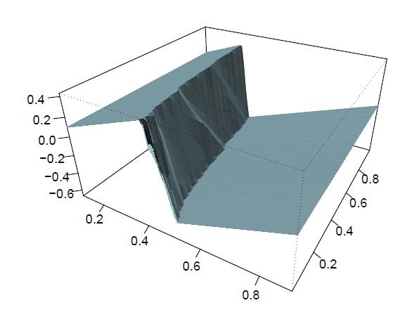
Note that the data perturbation technique requires fitting the quantile regression function multiple times for various $\tau$’s and $\lambda$’s, and thus can be computationally expensive. To further reduce the computation cost, the solution surface of the coefficient of $\hat{f}_{\lambda,\tau}({\bf x})$ with respect to $\lambda$ and $\tau$ can be constructed following Rosset (2009). In particular, Li et al. (2007) and Takeuchi et al. (2009) show that the solution path of $\hat{f}_{\lambda,\tau}({\bf x})$ is piecewise linear with respect to $\lambda$ (or $\tau$) when $\tau$ (or $\lambda$) is fixed; Rosset (2009) explores the bi-level path of regularized quantile regression and shows that the solution surface of $\hat{f}_{\lambda,\tau}({\bf x})$ can be efficiently constructed with respect to both $\lambda$ and $\tau$. The solution surface is mapped as a piecewise linear function of $\tau$ or $\lambda$ and the possible locations of the bi-level optima can be found in one run of the base algorithm. That being said, the coefficient of $\hat{f}_{\lambda,\tau}({\bf x})$ for various $\lambda$’s and $\tau$’s can be obtained at essentially the same computation cost as fitting one time of the base algorithm. Figure 1 displays $\hat{f}_{\tau,\lambda}({\bf x})$ for a fixed $\bf x$ as a function of $\lambda$ and $\tau$ in a randomly selected replication of the simulated Example 1.

The following technical assumptions are made.

Assumption 1. For any $\tau\in(0,1)$, there exists $\bar{f}_{\tau}\in{\cal F}$, such that $e(\bar{f}_{\tau},\tilde{f}^{*}_{\tau})\leq s_{n}$ for some positive sequence $s_{n}\rightarrow 0$ as $n\rightarrow\infty$.

This is analogous to Assumption 1 in Wang et al. (2008) and ensures that the true quantile regression function $\tilde{f}^{*}_{\tau}$ can be well approximated by ${\cal F}$.

Assumption 2. For any $\tau\in(0,1)$ and $f\in{\cal F}$, there exist constants $a_{1}>0$ and $0<\alpha\leq 1$ such that

Assumption 2 describes the local smoothness of $f({\bf x})$ within the neighborhood of $\tilde{f}^{*}_{\tau}({\bf x})$. Note that $e(f,\tilde{f}^{*}_{\tau})=E(h_{\tau}({\bf X},\tilde{Y}))$ with

by Lemma 4 in Li et al. (2007), so Assumption 2 is the same as Assumption A in Li et al. (2007).

Next we measures the cardinality of ${\cal F}$ by the $L_{2}$-metric entropy with bracketing. Given any $\epsilon>0$, $\{(f_{a}^{l},f_{a}^{u}),a=1,\ldots,A\}$ is an $\epsilon$-bracketing function set of ${\cal F}$ if for any $f\in{\cal F}$ there exists an $a$ such that $f_{a}^{l}\leq f\leq f_{a}^{u}$, and $\|f_{a}^{l}-f_{a}^{u}\|_{2}\leq\epsilon$ for all $a=1,\ldots,A$. The $L_{2}$-metric entropy with bracketing $H_{B}(\epsilon,{\cal F})$ is then defined as the logarithm of the cardinality of the smallest $\epsilon$-bracketing function set of ${\cal F}$. Denote ${\cal F}(k)=\{f\in{\cal F}:J(f)\leq k\}$, ${\cal F}_{\infty}=\{f\in{\cal F}:J(f)<\infty\}$ and $J_{0}=\min\limits_{\tau}\max\{J(\bar{f}_{\tau}),1\}$.

Assumption 3. For some positive constants $a_{2},a_{3}$ and $a_{4}$, there exists some $\epsilon_{n}>0$ such that

where $\phi(\epsilon_{n},k)=\frac{1}{D}\int_{a_{4}D}^{a_{3}^{1/2}D^{\alpha/2}}H_{B}^{1/2}(u,{\cal F}(k))du$ and $D=D(\epsilon_{n},\lambda,k)=\min\{\epsilon_{n}^{2}+(k-1)\lambda J_{0},1\}$.

To illustrate the asymptotic theory, a simple theoretic example is considered. Let ${\bf X}$ be sampled from a uniform distribution on $(0,3)$ and $Y\in\{1,2,3\}$ be sampled according to $p_{k}(x)=0.8$ if $k-1\leq x<k$ and 0.1 otherwise. Let ${\cal F}_{1}=\{f:f\in{\cal H}_{K},f(x)\in(0.5,3.5)\}$, where $K$ is the Gaussian kernel.

To verify Assumption 1, note that for any $\tau\in(0,1)$, $\tilde{f}^{*}_{\tau}(x)$ is continuous in $x$ except at $x=1$ and $x=2$. For given $s_{n}$, define

then $g_{\tau}(x)$ is a continuous function of $x$, and $\|g_{\tau}-\tilde{f}^{*}_{\tau}\|_{1}\leq s_{n}/2$. Furthermore, as $g_{\tau}(x)$ is continuous, Steinwart (2001) shows that there exists a $\bar{f}_{\tau}\in{\cal F}_{1}$ such that $\|g_{\tau}-\bar{f}_{\tau}\|_{1}\leq\|g_{\tau}-\bar{f}_{\tau}\|_{\infty}\leq s_{n}/2$. Therefore, $\|\bar{f}_{\tau}-\tilde{f}^{*}_{\tau}\|_{1}\leq\|g_{\tau}-\tilde{f}^{*}_{\tau}\|_{1}+\|g_{\tau}-\bar{f}_{\tau}\|_{1}\leq s_{n}$. Since $|\rho_{\tau}(y-\bar{f}_{\tau}(x))-\rho_{\tau}(y-\tilde{f}_{\tau}^{*}(x))|\leq|(y-\bar{f}_{\tau}(x))-(y-\tilde{f}_{\tau}^{*}(x))|=|\bar{f}_{\tau}(x)-\tilde{f}_{\tau}^{*}(x)|,$ then

To verify Assumption 2, note that $e(f,\tilde{f}_{\tau}^{*})=E(h_{\tau}(X,\tilde{Y}))=E\Big(E(h_{\tau}(X,\tilde{Y})|X)\Big)$, and

where $P_{X}(u)=p_{k}(X)$ if $k-0.5\leq u<k+0.5.$ Therefore, Assumption 2 is satisfied with $\alpha=0.5$ and $a_{1}=\sqrt{0.05}$.

To verify Assumption 3, since ${\cal H}_{B}(u,{\cal F}(k))=O(\log^{2}(k/u))$ (Zhou, 2002) for any given $k$ and $\phi(\epsilon_{n},k)$ is nonincreasing in $D$, there exist positive constants $c_{1},c_{2}$, such that

Without loss of generality, assume $s_{n}\leq\epsilon_{n}^{2}\leq 1$, and then $\delta_{n}^{2}=\epsilon_{n}^{2}$. Solving (9), yields that $\delta_{n}^{2}=O\Big((\frac{\log^{2}n}{n})^{1/(2-\alpha)}\Big)$, when $\lambda J_{0}\sim\delta_{n}^{2}$.

Finally, by Corollary 1, $E\|\hat{p}_{\lambda}-p\|_{1}=O\left(\frac{2}{m}+m^{2}a_{1}^{-1}n^{-1/3}(\log n)^{2/3}\right)$. This implies that $E\|\hat{p}_{\lambda}-p\|_{1}=O\big(n^{-1/9}(\log n)^{2/9}\big)$ when $m$ is set as $O\big(n^{1/9}(\log n)^{-2/9}\big)$.

Five simulated examples are generated for comparison.

Example 1. First, $Y$ is generated uniformly over $\{1,2,3,4,5\}$. Next, given $Y=y$, the covariates ${\bf X}$ are generated from $\text{T}(\mu(y),\Sigma,df=2)$, a multivariate $t$ distribution with $\mu(y)=(\cos(2y\pi/5),\sin(2y\pi/5))^{T}$, $\Sigma=diag(1,2)$ and degree of freedom 2. The training size is 400, and the testing size is 2600.

Example 2. First, $Y$ is generated uniformly over $\{1,2,\ldots,10\}$. Next, given $Y=y$, the covariates ${\bf X}$ are generated from $\text{T}(\mu(y),\Sigma,df=2)$, where $\mu(y)=(\cos(y\pi/5),\sin(y\pi/5))^{T}$ and $\Sigma=diag(1,2)$. The training size is 400, and the testing size is 2600.

Example 3. First, $Y$ is generated uniformly over $\{1,2,\ldots,20\}$. Next, given $Y=y$, the covariates ${\bf X}$ are generated from $\text{T}(\mu(y),\Sigma,df=2)$, where $\mu(y)=(\cos(y\pi/10),\sin(y\pi/10))^{T}$ and $\Sigma=diag(1,2)$. The training size is 400, and the testing size is 2600.

Example 4. First, $Y$ is generated uniformly over $\{1,2,3,4,5\}$. Next, given $Y=y$, the covariates ${\bf X}$ are generated from $\text{T}(\mu(y),\Sigma,df=2)$, where $\mu(y)=(\cos(2y\pi/5),\sin(2y\pi/5),$ $0,\ldots,0)^{T}$, and $\Sigma=diag(1,2,1,\ldots,1)$ if $y$ is odd and $\Sigma=diag(2,1,1,\ldots,1)$ if $y$ is even. The training size is 400, and the testing size is 2600.

Example 5. First, $Y$ is generated uniformly over $\{1,2,\ldots,10\}$. Next, given $Y=y$, the covariates ${\bf X}$ are generated from $\text{T}(\mu(y),\Sigma,df=2)$, where $\mu(y)=(\cos(y\pi/5),\sin(y\pi/5),$ $0,\ldots,0)^{T}$, and $\Sigma=diag(1,2,1,\ldots,1)$ if $y$ is odd and $\Sigma=diag(2,1,1,\ldots,1)$ if $y$ is even. The training size is 400, and the testing size is 2600.

Examples 1-3 are generated similarly, but with different number of classes $K$ and different mean vectors $\mu(y)$. When $K$ gets larger, the generated data from different classes become more overlapped and thus the resultant classification becomes more difficult. Examples 4 and 5 include additional noise variables and heteroscedastic covariance matrices. Each simulated example is repeated 50 times, and the averaged test errors and the corresponding standard deviations are reported in Table 1.

Evidently, the proposed estimation method delivers superior numerical performance, and outperforms BLM, TREE and WMC in all the examples. As a model-free method, WMC yields competitive performance in Example 1 and Example 4 with $K=5$ where the data from different classes are relatively far apart leading to clear-cut classification boundary. However, when $K$ gets larger, WMC requires much more intensive computing power, and its numerical performance appears to be less satisfactory in Examples 2 and 5 with $K=10$. Furthermore, the performance of WMC in Example 3 with $K=20$ is not reported in Table 1, since it is computationally expensive to achieve reasonably good estimation accuracy.

In this section, the proposed multiclass probability estimation method is applied to the iris data, the white wine quality data and the abalone data. All datasets are publicly available at the University of California Irvine Machine Learning Repository (http://archive.ics.uci.edu/ml/).

The iris data has 4 continuous attributes: sepal length, sepal width, petal length, and petal width, and three classes: Setosa, Versicolour, and Virginica. The size of the iris dataset is 150, and each class has 50 observations. We randomly select 30 observations from each class and set as the training set, and the remaining 60 observations are used for testing. The white wine quality data has 11 attributes, which characterize various aspects of the white wines, and the response ranges from 0 to 10 representing quality scores made by wine experts. For illustration, we focus only on three classes with quality scores 5, 6 and 7, and a total of 4535 white wines are selected, where 1457, 2198 and 880 white wines score 5, 6 and 7, respectively. We randomly select 100 white wines from each class as the training set, and the remaining 4235 white wines are used for testing. The abalone data has 8 attributes on various physical measurements of an abalone, and 29 classes representing different ages of an abalone. Since some extreme classes have very few abalones, we only focus on the $K$ largest classes with $K=5,8,10$. In specific, for $K=5$, classes $7-11$ are selected with a total of 2768 abalones; for $K=8$, classes $6-13$ are selected with a total of 3498 abalones; for $K=10$, classes $5-14$ are selected with a total of 3739 abalones. In all scenarios, we randomly select 50 abalones from each class as the training set, and keep the remaining abalones for testing.

Note that the true conditional probability $p_{k}({\bf x})$ is not available in the real applications, so only CEE is computed and used for comparison. In addition, we also compare the averaged misclassification error (MCE) of each probability estimation method on the testing set, where the classification label is predicted as $\hat{y}_{t}=\mathop{\rm argmax}_{k}\hat{p}_{k}({\bf x}_{t})$, and MCE is defined as

The averaged CEE and MCE over 50 replications are reported in Table 2.

It is evident that the proposed probability estimation method delivers competitive results against other competitors. It yields the smallest CEE and MCE in all real examples, except that WMC produces slightly smaller CEE in the iris example. The performance of WMC is not reported for the abalone example with $K=8$ and $10$ due to the computational burden.

References

- [1] Bondell, H., Reich, B. and Wang, H. (2010). Non-crossing quantile regression curve estimation, Biometrika, 97, 825-838.
- [2] Breiman, L. (1992). The little bootstrap and other methods for dimensionality selection in regression: -fixed Prediction Error, Journal of the American Statistical Association, 87, 738-754.
- [3] Breiman, L. and Spector, P. (1992). Submodel selection and evaluation in regression - the - random case, International Statistical Review, 3, 291-319.
- [4] Breiman, L. (1996). Heuristics of instability and stabilization in model selection, Annals of Statistics , 26, 801-849.
- [5] Chen, J. and Lazar, N. (2010). Quantile estimation for discrete data via empirical likelihood, Journal of Nonparametric Statistics, 22, 237-255.
- [6] Efron, B. (2004). The estimation of prediction error: covariance penalties and cross-validation, Journal of the American Statistical Association, 99, 619-632.
- [7] Gu, C. (2002). Smoothing spline ANOVA models, New York: Springer-Verlag.
- [8] Hansen, B. (2004). Nonparametric conditional density estimation, Unpublished manuscript.
- [9] Hastie, T. and Tibshirani, R. (1998). Classification by pairwise coupling, The Annals of Statistics, 26, 451-471.
- [10] He, X. (1997). Quantile curves without crossing, The American Statistician, 51, 186-192.
- [11] He, X., Ng, P. and Portnoy S. (1998). Bivariate quantile smoothing splines, Journal of the Royal Statistical Society, Series B, 60, 537-550.
- [12] Kimeldorf, G. and Wahba, G. (1971). Some results on Tchebycheffian spline functions, Journal of Mathematical Analysis and Applications, 33, 82-95.
- [13] Koenker, R. (2005). Quantile regression, New York: Cambridge University Press.
- [14] Koenker, R. and Bassett, G. (1978). Regression quantiles, Econometrica, 46, 33-50.
- [15] Lee, Y., Lin, Y. and Wahba, G. (2004). Multicategory support vector machines, theory, and application to the classification of micoarray data and satellite radiance data, Journal of the American Statistical Association, 99, 67-81.
- [16] Li, Y., Liu, Y. and Zhu, J. (2007). Quantile regression in reproducing kernel Hilbert spaces, Journal of the American Statistical Association, 102, 255-268.
- [17] Liu, Y. and Wu, Y. (2011). Simultaneous multiple non-crossing quantile regression estimation using kernel constraints, Journal of Nonparametric Statistics, 23, 415-437.
- [18] Liu, Y., Zhang, H. H. and Wu, Y. (2011). Soft and hard classification? Large-margin unified machines, Journal of the American Statistical Association, 106, 166-177.
- [19] Machado, J. and Santos Silva, J. (2005). Quantiles for counts, Journal of American Statistical Association, 100, 1226-1237.
- [20] Rosset, S. (2009). Bi-level path following for cross validated solution of kernel quantile regression, Journal of Machine Learning Research, 10, 2473-2505.
- [21] Shen, X. and Huang, H. (2006). Optimal model assessment, selection, and combination, Journal of the American Statistical Association, 101, 554-568.
- [22] Shen, X. and Wong, W. (1994). Convergence rate of sieve estimates, Annals of Statistics, 22, 580-615.
- [23] Takeuchi, I., Le, Q. and Sears, T. (2009). Nonparametric conditional density estimation using piecewise-linear solution path of kernel quantile regression. Neural Computation, 21, 533-559.
- [24] Wahba, G. (1990). Spline models for observational data, Philadelphia: SIAM.
- [25] Wahba, G. (2002). Soft and hard classification by reproducing kernel Hilbert space methods. In Proceedings of the National Academy of Sciences, 16524-16530.
- [26] Wang, H., Zhu, Z., and Zhou, J. (2009). Quantile regression in partially linear varying coefficient models, Annals of Statistics, 37, 3841-3866.
- [27] Wang, J. and Shen, X. (2006). Estimation of generalization error: random and fixed inputs, Statistica Sinica, 16, 569-588.
- [28] Wang, J., Shen, X. and Liu, Y. (2008). Probability estimation for large margin classifiers, Biometrika, 95, 149-167.
- [29] Wu, T., Lin, C. and Weng.R. (2004). Probability estimates for multi-class classification by pairwise coupling, Journal of Machine Learning Research, 5, 975-1005.
- [30] Wu, Y., Zhang, H. and Liu, Y. (2010). Robust model-free multiclass probability estimation, Journal of the American Statistical Association, 105, 424-436.
- [31] Wu, Y. and Liu, Y. (2009). Stepwise multiple quantile regression estimation using non-crossing constraints, Statistics and Its Interface, 2, 299-310.
- [32] Xu, M., Watanachaturaporn, P., Varshney, P and Arora, M. (2005). Decision tree regression for soft classification of remote sensing data, Remote Sensing of Environment, 97, 322-336.
- [33] Yang, Y. and He, X. (2012). Bayesian empirical likelihood for quantile regression, The Annals of Statistics, 40, 1102-1131.
- [34] Yu, K., Lu, Z. and Stander, J. (2003). Quantile regression: applications and current research areas, The Statistician, 52, 331-350.
- [35] Zhou, D. (2002). The covering number in learning theory, Journal of Complexity, 18, 739-767.