Performance Analysis of Error Control Coding Techniques for Peak-to-Average Power Ratio Reduction of Multicarrier Signals

With the progressive development of mobile cellular communication technology, the need for multi use services and broadband convergence of voice, data, videos and automated applications in a single device has become obvious. To support these applications there is increasing demand for high bit rate and reliable wireless communication system which has led to many new emerging modulation techniques. One of such techniques is Orthogonal Frequency Division Multiplexing (OFDM). OFDM has emerged as an efficient multicarrier modulation scheme for wireless, frequency selective communication channels. OFDM is a method of transmitting data simultaneously over multiple, equally spaced carrier frequencies using the Fourier transform processing for modulation and demodulation [1]. This method has been proposed or adopted for various types of radio systems such as DAB,DVB [2][3] and WLAN [4]. Specifically, the OFDM is preferred in most of the high bandwidth, spectrally efficient transmission system due to its robustness in multipath fading environments and hence its effective resistance to inter symbol interference (ISI). It is worth to note that ISI is the single most important factor which limits the maximum bit rate of wireless transmission system, especially in multipath environments.

While OFDM is a promising technology, the principal difficulty encountered in its practical realizations is that, it exhibits a very high peak-to-average power ratio (PAPR). This is due to the summation of the subcarriers, which could get added constructively or destructively depending on the data being transmitted in parallel. This creates large variations between the average and the peak signal power in OFDM systems. Due to this high PAPR, RF power amplifier should be operated in a very large linear region for if not, the signal peak might get into the non-linear region of the power amplifier causing undesirable signal distortion. The operation of the power amplifiers with a very large linear region leads to expensive transmitter and receiver systems. The signal distortion introduced can result in inter modulation noise among the subcarriers and out of band radiation[5]. Furthermore, if battery power is a constraint, as it is the case with portable equipment, then the power amplifier is required to behave linearly up to peak envelope power and hence must be operated inefficiently. Digital hard limiting of the transmitted signal has been shown to alleviate this problem[6] but only at the cost of spectral side lobe growth and consequent performance degradation.

This leads to the motivation to explore and find other ways to control PAPR of the transmitted signal without compromising the performance of the OFDM systems. A promising method, which has attracted considerable attention, is the use of Error Control Coding (ECC) techniques. The technique of using ECC to counter PAPR, introduced first in[7] and later developed in [8] uses block coding to transmit data across the carriers in such a way that only those polyphase sequences which have low PAPR are selected.Though many ECC based methods [9][10][11] have been proposed to date in the literature for PAPR reduction, until now there has been no comparative study of PAPR reduction capability of various channel coding techniques which is a major gap in the research in this area.The objective of this paper is to fill this gap and investigate the PAPR reduction performance for OFDM signal using various channel coding techniques.

The organization of this paper is as follows. In section 2,the model for OFDM signal and its PAPR is discussed. In section 3, PAPR analysis of BPSK modulated OFDM signal is discussed. Section 4 gives notation which has been used throughout section 5. In section 5, various types of linear block codes has been discussed. In section 6, simulation results and its discussion is given. Finally section 7 concludes the paper.

For our analysis emphasis is on examining the PAPR of an OFDM signal. Therefore, the OFDM system model used in this paper is a simplified version of the practical OFDM model. Specifically, we have ignored the guard interval because it does not contribute to the PAPR [12]. Assuming that any pulse shaping in the transmitter is flat over all of the subcarriers, and deal only with the PAPR of the baseband signal. For one OFDM symbol with N subcarriers, the normalized complex baseband signal can be written as:

$$s(t)=\frac{1}{\sqrt{N}}\sum_{k=0}^{N-1}c_{k}e^{\frac{j2\pi kt}{T}}\qquad 0\leq t\leq T$$

(1)

where $c_{k}$ is the frequency domain information symbol mapped to the $k_{th}$ subcarrier of the OFDM symbol and $T$ is the OFDM symbol duration. The peak-to-average power ratio (PAPR) of the given frequency domain samples,
$c=\{c_{0},c_{1},c_{2},\cdots,c_{N-1}\}$ is defined as:

$$PAPR\triangleq\stackrel{{\scriptstyle max}}{{0\leq t\leq T}}\frac{\left|s(t)\right|^{2}}{E[\left|s(t)\right|^{2}]}$$

(2)

where $E[.]$ denotes a time averaging operator. The distribution of PAPR values is described using the complementary cumulative distribution function (CCDF). The CCDF of the PAPR represents the probability that the PAPR of a data block exceed a given threshold, $\xi$ and is given [13] by

$$Pr(PAPR>\xi)=1-(1-e^{-\xi})^{N}.$$

(3)

For the sake of simplicity we have considered BPSK modulation. PAPR analysis of BPSK modulated OFDM signal is done to understand the reason behind high PAPR. For BPSK modulated OFDM signal, $c_{k}\in\{-1,+1\}$. Using the technique as described in [14] and assuming $T=1.0$ equation (1) can be written as:

	$\displaystyle\sqrt{N}s(t)$	$\displaystyle=$	$\displaystyle\sum_{k=0}^{N-1}c_{k}e^{j2\pi kt}$
	$\displaystyle N\left|s(t)\right|^{2}$	$\displaystyle=$	$\displaystyle\Big(\sum_{k=0}^{N-1}c_{k}e^{j2\pi kt}\Big)^{2}$		(4)
		$\displaystyle=$	$\displaystyle\Big(\Re\big[\sum_{k=0}^{N-1}c_{k}e^{j2\pi kt}\big]\Big)^{2}+\Big(\Im\big[\sum_{k=0}^{N-1}c_{k}e^{j2\pi kt}\big]\Big)^{2}$
		$\displaystyle=$	$\displaystyle\Big(\sum_{k=0}^{N-1}c_{k}\cos(2\pi kt)\Big)^{2}+\Big(\sum_{k=0}^{N-1}c_{k}\sin(2\pi kt)\Big)^{2}$
		$\displaystyle=$	$\displaystyle\sum_{k=0}^{N-1}c_{k}^{2}\cos^{2}(2\pi kt)+{}$
			$\displaystyle{}+2\sum_{k=0}^{N-2}\sum_{i=k+1}^{N-1}c_{k}c_{i}\cos(2\pi kt)\cos(2\pi it)+{}$
			$\displaystyle{}+\sum_{K=0}^{N-1}c_{k}^{2}\sin^{2}(2\pi kt)+{}$
			$\displaystyle{}+2\sum_{k=0}^{N-2}\sum_{i=k+1}^{N-1}c_{k}c_{i}\sin(2\pi kt)\sin(2\pi it)$
		$\displaystyle=$	$\displaystyle N+2\sum_{k=0}^{N-2}\sum_{i=k+1}^{N-1}c_{k}c_{i}\cos(2\pi(i-k)t)$
		$\displaystyle=$	$\displaystyle N+2P_{0}(t)$

where $\Re[x]$ and $\Im[x]$ are the real and imaginary parts of $x$ respectively and the AC component of the power envelope of the OFDM signal $P_{o}(t)$ is defined as:

$$P_{0}(t)=\sum_{k=0}^{N-2}\sum_{i=k+1}^{N-1}c_{k}c_{i}\cos(2\pi(i-k)t).$$

(5)

The double summation in (5) can be replaced with a single summation by combining each term to its harmonic and $P_{0}(t)$ becomes:

$$P_{0}(t)=\sum_{k=1}^{N-1}C_{k}\cos(2\pi kt)$$

(6)

which can be physically interpreted as the sum of cosine harmonics weighted by the aperiodic autocorrelation $C_{k}$ of the frequency domain information bits, where the aperiodic autocorrelation $C_{k}$ is defined as:

$$C_{k}=\sum_{i=0}^{N-k-1}c_{i}c_{i+k}.$$

(7)

Substituting for $P_{0}(t)$ from (6) in (4), the average power of $s(t)$ becomes:

	$\displaystyle E[\left|s(t)\right|^{2}]$	$\displaystyle=$	$\displaystyle E\big[1+\frac{2P_{0}(t)}{N}\big]$		(8)
		$\displaystyle=$	$\displaystyle 1+\frac{1}{N}E[2P_{0}(t)]$
		$\displaystyle=$	$\displaystyle 1.$

As the average power of $s(t)$ is unity, the PAPR in (2), when considering its symmetry with respect to the half symbol time becomes:

$$PAPR=\stackrel{{\scriptstyle max}}{{0\leq t\leq 0.5}}\big(1+\frac{2}{N}P_{0}(t)\big)$$

(9)

where $P_{0}(t)$ is given by (6). From (6), (7) and (9), it is found that the PAPR is completely characterized by the aperiodic autocorrelations $C_{k}$. Without any loss of generality we can extend this analysis to other efficient modulation techniques such as QPSK/QAM.

For the $N=4$ the aperiodic autocorrelation $C_{k}$ are given by:

	$\displaystyle C_{1}$	$\displaystyle=$	$\displaystyle c_{0}c_{1}+c_{1}c_{2}+c_{2}c_{3}$
	$\displaystyle C_{2}$	$\displaystyle=$	$\displaystyle c_{0}c_{2}+c_{1}c_{3}$
	$\displaystyle C_{3}$	$\displaystyle=$	$\displaystyle c_{0}c_{3}.$

Now there is a need to reduce the aperiodic correlation among the subcarriers so that PAPR is reduced. There are various method to do this such as scrambling [15], here we have focused only on the linear error control coding techniques. By employing error control coding techniques it gives dual advantage of error control as well as PAPR reduction. Next sections briefs about various error control codes considered for PAPR reduction.

We have considered codes over some alphabet $\mathcal{A}$ and reserved the letter $q$ to represent the cardinality of $\mathcal{A}$. In this paper only binary codes have been considered so $q=2$ and $\mathcal{A}=\{0,1\}$. A code $C$ is a subset of $\mathcal{A}^{n}$ for some positive integer $n$. There are four fundamental parameters associated with a code $C$:

• •

  Its block length: $n$, where $n\subseteq\mathcal{A}^{n}$

• •

  Its message length: $k=\log_{q}|C|$

• •

  Its minimum distance: $d_{min}$, which is defined as the the number of coordinates where $c_{1}$ & $c_{2}$ differ, here $c_{1},c_{2}\in C$

• •

  Its alphabet size,$q=|\mathcal{A}|$

A code is often characterized by four parameters it achieves and such code is referred as an $[n,k,d]_{q}$ code. Bold face letters represents matrices.

There are various ways to specify a code but the most convenient way is to give an encoding function, thereby specifying how to create arbitrary code words. This generalized mapping can be used to describe classes of codes in a succinct manner. In this paper, we have considered a special class of codes called linear codes.
Liner codes are obtained when the alphabet $\mathcal{A}$ is associated with the field $\mathbb{F}_{q}$ for some finite value of $q$. In such a case $\mathcal{A}^{n}$ contains the code words and received words as a vector space.

When a code $C\subseteq\mathbb{F}^{n}_{q}$ is a linear subspace of $\mathbb{F}^{n}_{q}$, then the code is called a linear code.

A simplified diagram of OFDM Transmitter and Receiver used for our study is shown in Fig.2. The presented simulations has been performed for IEEE 802.11a standard (i.e N=64) modulated with 16 QAM. The statistics of peak and instantaneous power of OFDM symbols generated with a text as an input has been investigated with different channel coding techniques.

The complementary cumulative distribution function (CCDF) has been used here to assess the PAPR reduction performance of the coded OFDM using various channel coding techniques against uncoded OFDM. The CCDF of the PAPR denotes the probability that the PAPR of the data block exceeds a given threshold $\xi$. The CCDF is given by (3). In all the simulations, value of PAPR has been studied for $CCDF=10^{-2}$. Result of Hamming coded OFDM simulation is tabulated in Table.1 and CCDF vs PAPR plot is shown in Fig.3. From Fig.3, it is observed that Hamming Codes helps in reducing PAPR and maximum PAPR reduction has been observed for $m=6$.

From Fig.4 and Table.2, it is observed that PAPR reduction performance of cyclic code is slightly better than the Hamming code and the maximum PAPR reduction has been obtained for $m=4$.

The connection vectors or polynomial generators of a convolutional code are usually selected based on the code’s free distance property [17]. The first criterion is to select a code that does not have catastrophic error propagation and that has the maximum free distance for the given rate and constraint length. Then the number of paths at the free distance or the number of data bit errors the path represents should be minimized. For our investigation, we have referred a list of the best known code of rate $\frac{1}{2}$, K=3 to 14, and rate 1/3, K=3 to 14, which was compiled by Odenwalder [20] based on the above criteria. Generator vectors of the convolution codes are listed in octal form in Table.3 [17].

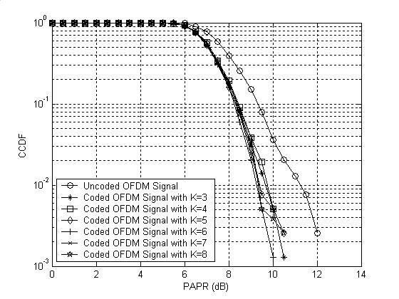
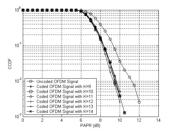
Fig.5 and 6 shows CCDF vs. PAPR curve of direct OFDM signal along with CCDF vs. PAPR curve for convolutionally coded OFDM signal with code rate 1/2 and different values of constraint length K. From Fig.5, it is observed that the PAPR reduction with convolution code is further better than the cyclic codes. Here the performance of convolution code with rate 1/2 and of different constraint length, from K=3 to 14 has been investigated. It has been observed that there is reduction of PAPR by more than $1.5$ dB for all the value of $K$ and the maximum reduction is observed for $K=6$. The results of simulation has been tabulated in Table.4.

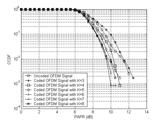
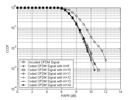
Fig.7 and 8 shows CCDF versus PAPR curve of direct OFDM signal along with CCDF vs. PAPR curve for convolutionally coded OFDM signal with code rate 1/3 and different values of constraint length K. The performance of convolution code with rate 1/3 and of different constraint length, from K=3 to 14 has been investigated. It has been observed that there is reduction of PAPR by more than $1$ dB for all the value of $K$ and the maximum reduction is observed for $K=9$. The results of simulation has been tabulated in Table.5. Furthermore from Table.4 and Table.5, it can be inferred that the PAPR reduction performance of convolution code with rate 1/2 is slightly better and less complex from implementation perspective than the convolution code with rate 1/3.

Fig.9 shows the CCDF vs PAPR curve of [23,12,7] and [24,12,8] Golay coded OFDM signal. From Fig.9, it can be easily inferred that the PAPR reduction performance of [23,12,7] Golay coded OFDM is better than the [24,12,8] Golay coded OFDM signal and the PAPR reduction is approximately 2 dB.

Fig.10 and 11 shows the CCDF vs PAPR curve for Reed-Muller coded OFDM signal with different values of $r$ and $m$ and the result of simulation has been tabulated in Table.6. From Table.6, it is observed that the maximum PAPR reduction obtained is equal to 2.2362 dB for $r=1$ and $m=4$. The PAPR reduction performance of Reed-Muller code is better than the Golay code as evident from Figs.9,10 and 11.

Fig.12 shows the PAPR reduction performance of various channel coding techniques considered namely,Hamming code, cyclic code, convolutional code with rate 1/2 and 1/3 respectively,Golay code and Reed-Muller code. The PAPR reduction performance of all the considered channel coding techniques has been tabulated in Table.7. From Table.7 it can be easily inferred that the PAPR reduction performance of Reed-Muller code is better than the other considered codes.

From Table.7, it is clear that the use of channel coding for OFDM signal reduces the aperiodic autocorrelation between OFDM symbols on subcarriers as a result of which PAPR of the coded OFDM signal reduces though to a very small extent at most by 2 dB. This fact is the direct result of equation(5). The channel coding techniques can be arranged in the following order based on their PAPR reduction performance:

1. 1.

   Reed-Muller code with $r=1$ and $m=4$

2. 2.

   Convolution code, with rate 1/2 and K=6

3. 3.

   $[23,12,7]$ Golay code

4. 4.

   Convolution code, with rate 1/3 and K=9

5. 5.

   Cyclic code with m=4

6. 6.

   Hamming code with m=6.

OFDM is one of the promising multicarrier modulation technique which offer very high data rates over the wireless medium without getting affected by ISI and fading over the wireless medium.

In this paper, we have analyzed the PAPR of BPSK modulated OFDM signal. As an outcome of the analysis, it is found that the PAPR is completely characterized by the aperiodic autocorrelation of OFDM symbols on subcarriers.

To reduce the aperiodic autocorrelation of OFDM symbol on subcarriers, we have used various channel coding techniques; especially linear block codes such as Hamming code, cyclic code, convolution code, Golay code and Reed-Muller codes, for the OFDM signal. As a result of this we have compared the PAPR reduction performance of the considered channel codes and found that the PAPR reduction performance of Reed-Muller code with $r=1$ and $m=4$ is the best among the considered channel codes. Moreover, from the perspective of hardware complexity of encoder and decoder, PAPR reduction performance of convolution code is found to be optimum as compared to other channel coding techniques. Though the reduction in PAPR achieved is at most 2 dB, one of the major advantages of the discussed study is that it can be combined with selective mapping (SLM) or other conventional PAPR reduction techniques for further reduction in PAPR.

References

- [1] M. Nakhai, “Multicarrier transmission,” Signal Processing, IET, vol. 2, no. 1, pp. 1 –14, march 2008.
- [2] H. Gacanin and F. Adachi, “A comprehensive performance comparison of ofdm/tdm using mmse-fde and conventional ofdm,” in Vehicular Technology Conference, 2008. VTC Spring 2008. IEEE, may 2008, pp. 1404 –1408.
- [3] , “Broadband radio access networks (bran);hiperlan type 2;data link control (dlc) layer part 1: Basic data transport functions,” [Available Online] http://www.etsi.org/deliver/etsi_ts/101700_101799/10176101/01.01.01_60/ts_10176101v010101p.pdf, 2000.
- [4] IEEE, “Draft supplement to standard for telecommunications and information exchange between systems-lan/man specific requirements-part 11: Wireless mac and phy specifications: High speed physical layer in the 5 ghz band, ieee802.11,” IEEE, Tech. Rep. P802.11a/D6.0(1999), May 1999.
- [5] H. Ochiai and H. Imai, “Performance of block codes with peak power reduction for indoor multicarrier systems,” in Vehicular Technology Conference, 1998. VTC 98. 48th IEEE, vol. 1, may 1998, pp. 338 –342 vol.1.
- [6] X. Li and J. Cimini, L.J., “Effects of clipping and filtering on the performance of ofdm,” Communications Letters, IEEE, vol. 2, no. 5, pp. 131 –133, may 1998.
- [7] A. Jones, T. Wilkinson, and S. Barton, “Block coding scheme for reduction of peak to mean envelope power ratio of multicarrier transmission schemes,” Electronics Letters, vol. 30, no. 25, pp. 2098 –2099, dec 1994.
- [8] T. Wilkinson and A. Jones, “Minimisation of the peak to mean envelope power ratio of multicarrier transmission schemes by block coding,” in Vehicular Technology Conference, 1995 IEEE 45th, vol. 2, jul 1995, pp. 825 –829 vol.2.
- [9] C.-Y. Chen, C.-H. Wang, and C. chao Chao, “Convolutional codes for peak-to-average power ratio reduction in ofdm,” in Information Theory, 2003. Proceedings. IEEE International Symposium on, june-4 july 2003, p. 5.
- [10] J. Davis and J. Jedwab, “Peak-to-mean power control in ofdm, golay complementary sequences, and reed-muller codes,” Information Theory, IEEE Transactions on, vol. 45, no. 7, pp. 2397 –2417, nov 1999.
- [11] K. Paterson and V. Tarokh, “On the existence and construction of good codes with low peak-to-average power ratios,” in Information Theory, 2000. Proceedings. IEEE International Symposium on, 2000, p. 217.
- [12] J. Tellado, Multicarrier Modulation with Low PAR: Applications to DSL and Wireless. Boston: Kluwer Academic Publisher, 2000.
- [13] R. Nee and R.Prasad, OFDM for Wireless Multimedia Communications. Artech House, 2000.
- [14] S. Narahashi and T. Nojima, “New phasing scheme of n-multiple carriers for reducing peak-to-average power ratio,” Electronics Letters, vol. 30, no. 17, pp. 1382 –1383, aug 1994.
- [15] M. K. Sanjay Singh and H. Mruthyunjaya, “Reduction of peak-to-average power ratio of an ofdm signal using scrambling coding,” International Journal of Computer Science and Communication Technology, vol. 1, no. 2, pp. 109–115, 2009.
- [16] S. Lin and D. J. Jr., Error Control Coding: Fundamentals and Applications. Upper Saddle River, New Jersey: Prentice Hall, 2004.
- [17] J. Proakis, Digital Communications, 4th ed. New York: McGraw-Hill, 2001.
- [18] M. T. E. Golay, “Multi-slit spectrometry,” J. Opt. Soc. Am., vol. 39, no. 6, pp. 437–437, Jun 1949. [Online]. Available: http://www.opticsinfobase.org/abstract.cfm?URI=josa-39-6-437
- [19] F. J. MacWilliams and N. J. A. Sloane, The Theory of Error Correcting Codes, 1st ed. Amsterdam: Elsevier Science, 1977.
- [20] J. P. Odenwalder, Error Control Coding Handbook. San Diego, California: Linkabit Corporation, 1976.