Classification of Flat Virtual Pure Tangles
Abstract.
Virtual knot theory, introduced by Kauffman [Kau], is a generalization of classical knot theory of interest because its finite-type invariant theory is potentially a topological interpretation [BN1] of Etingof and Kazhdan’s theory of quantization of Lie bi-algebras [EK]. Classical knots inject into virtual knots [Ku], and flat virtual knots [Ma1, Ma2] is the quotient of virtual knots which equates the real positive and negative crossings, and in this sense is complementary to classical knot theory within virtual knot theory.
We completely classify flat virtual tangles with no closed components (pure tangles). This classification can be used as an invariant on virtual pure tangles and virtual braids.
Key words and phrases:
knots, virtual knots, flat virtual knots, flat knots, Reidemeister moves, finite-type invariants, Polyak algebra, associated graded, triangular group, quasi-triangular group, quantum invariants, quantum group1991 Mathematics Subject Classification
57M25Acknowledgments
I am indebted to my PhD advisor Dror Bar-Natan for the computational evidence [BHLR] and conjecture on the main results of this paper, the idea of using the finger move in the first proof, on top of his generosity with his time, resources, care, and countless hours of inspiring discussion.
I am very grateful for the generous encouragements that other mentors have shown me, in particular Joel Kamnitzer, Louis Kauffman, and Vassily Manturov.
I am grateful for mathematical discussion with P. Lee, Z. Dancso, L. Leung, I. Halacheva, J. Archibald. In particular, P. Lee pointed out [BEER] which helped me understand more about flat virtual braids, known as the “triangular group” in the paper. I first learned about flat virtual knots in a lecture by Vassily Manturov in the Trieste summer school on knot theory.
1. Introduction
We study virtual knots because they are a natural generalization of classical knots into which classical knots inject, and more interestingly, because the -matrix invariants on classical knots extend naturally to virtual knots (or at least a variant of them).
We will define virtual knots by first recalling the definition of classical knots and generalize from it. Classical knots can be defined combinatorially as knots diagrams modulo Reidemeister moves. Knot diagrams are planar directed graphs with “crossings” as vertices. Crossings are special tetravalent vertices whose half-edges are cyclically-ordered and directed such that opposite pairs are “in-out” pairs. The crossings have exactly the combinatorial information to be represented as follows:
![[Uncaptioned image]](1209.4589v1/UsualCrossings.png)
The Reidemeister moves are local planar graph equivalence relations shown below where each skeleton strand can be oriented either way.
![[Uncaptioned image]](1209.4589v1/RMove.png)
Virtual knots have the same definition except with word “planar” omitted, i.e. virtual knot diagrams are (not-necessarily planar) graphs with crossings as vertices, and virtual knots are equivalence classes of virtual knot diagrams under the Reidemeister relations as local graph relations. Now, when not-necessarily planar graphs are drawn (or immersed) on the plane, transverse intersections of edges of the graph may occur. These are not vertices of the graph, but rather artifacts of drawing a non-planar graph on the plane, and are called “virtual crossings.” Here is a virtual knot diagram drawn in two different ways on the plane where the real crossings are circled and the other intersections are virtual crossings:
![[Uncaptioned image]](1209.4589v1/VirtualKnotDiagram.png)
Similarly, the strand between any two crossings in a Reidemeister relation may intersect other strands in the virtual knot diagram when drawn on the plane and have virtual crossings on them.
A natural question arises: how much bigger are virtual knots than classical knots? This leads to the consideration of the quotient of virtual knots by the crossing-flip relation which equates the (real) positive and negative crossings:
![[Uncaptioned image]](1209.4589v1/CrossingFlip.png)
in which all classical knots are equivalent to the unknot. This quotient is called flat virtual knots.
The subject of this paper is flat virtual long knots, where “long” simply refers to the skeleton of the knot being a long line, and the “skeleton” is the union of lines and/or circles obtained from tracing the knot diagram along the direction of the edges, across paired half-edges at crossings and forgetting the crossings.
In fact, flat virtual long knots are equivalent to descending virtual long knots, the subset of virtual long knots with only crossings whose over strand is earlier w.r.t. to the orientation of the skeleton than the under strand. This is because while virtual long knots project onto flat virtual long knots, there is a well-defined section map from flat virtual long knot back into virtual long knot, namely by sending any flat real crossing to a descending crossing, and the image of such a section map is exactly the descending virtual long knots. Notice descendingness of a crossing is not defined for round virtual knots, and the map that sends any flat crossing to a positive crossing is well-defined.
Our main result is the classification of both the “framed” and “unframed” versions of descending virtual long knots, where “framed” means the Reidemeister relation is not imposed and “unframed” means otherwise. We give a canonical representative for each equivalent class of descending virtual long knot diagrams under the Reidemeister moves.
Theorem 1.1 (Classification of Long Descending Virtual Knots, conjectured by Bar-Natan).
Framed descending virtual long knots are in bijection with the set of canonical diagrams . A canonical diagram is a descending virtual long knot diagram whose skeleton strand has a point before which it is the over strand in any crossing it participates in, and after which as the under strand, and does not contain bigons bounded by opposite signed crossings. An example is given in figure 1 and the general form is shown in figure 2.
Furthermore, is in bijection with the set of all “signed reduced permutations”, where a signed permutation is a set map which projects to the first components as a permutation, and a reduced signed permutation satisfies the extra condition that the image of pairs of consecutive numbers are not pairs of consecutive numbers with opposite signs, i.e. not , or for all .
Long unframed flat virtual knots are in bijection with the subset of with no “R1 kinks,” also shown in 2. See figure 3 for a list of canonical diagrams up to three crossings.
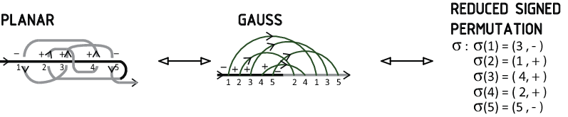


The above result can be generalized easily to the multi-strand case. We call flat virtual tangles whose skeleton is an ordered union of strands (in particular no closed loops) flat virtual pure tangles. Similar to the long knot case, these are again equivalent to descending virtual pure tangles.
Theorem 1.2 (Classification of Descending Virtual Pure Tangles).
Framed descending virtual pure tangles of strands are in bijection with the set of canonical diagrams , which are characterized by the same two conditions as in the one strand case in theorem 1.1 but applied to all strands. Unframed descending virtual pure tangles are in bijection with the subset of with no “R-I kinks”. See figure 4 for an example, and figure 5 for a partial list of canonical diagrams of descending virtual pure tangles on two strands up to two crossings.
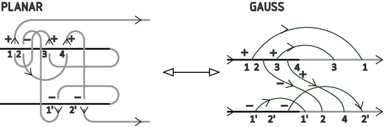

The proofs of both theorems are similar and amount to showing that a well-defined sorting map exists. For an example of the sorting, see figure 1.
This classification can be use as an invariant on virtual long knots and pure tangles, as well as virtual braids. If flat virtual braids inject into the pure tangles, then we have also obtained their classification.
2. Classification of Pure Descending Virtual Tangles
Having established that flat virtual pure tangles are equivalent to descending virtual pure tangles in the introduction,we present in this section the classification of descending virtual pure tangles and its proof. We will prove the classification for the framed version (see page 1.1) first, and then modify it slight for the unframed version to include Reidemeister 1.
2.1. Generic Diagrams of Pure Descending Virtual Tangles
In this subsection, we describe the generic form of pure descending virtual tangle diagrams. First, a few definitions to describe the diagrams:
Definition 2.1.
An interval of the skeleton of a pure descending virtual tangle is called an over (resp. under) interval if all of its subintervals that take part in crossings are the over strands in the crossings. A maximal over (resp. maximal under) interval is an over (resp. under) interval preceded and followed immediately by an under (resp. over) interval or by the beginning or end of the strand. An illegal interval is an interval consisting of first a maximal under interval and then a maximal over interval. These are illustrated below in Figure 6.
Convention 2.2.
All real crossings are descending all virtual crossings are neither over or under and not circled. The over interval of a crossing is drawn in black and the under interval drawn in grey. An interval not explicitly oriented means it can be oriented either ways. In any Gauss diagram, an unsigned Gauss arrow means it can have either sign. A “thick band” represents multiple strands or arrows, as in figure 6.

Generically, a pure descending virtual long knot diagram has multiple maximal over and under intervals. Due to descendingness, it always (as long as there is at least one crossing) starts with a maximal over and ends with a maximal under interval, while in between it alternates between over and under while having each maximal under interval only under the maximal over intervals before it. Thus, a generic diagram has illegal intervals on its skeleton. See figure 7 for an example. A generic descending virtual pure tangle diagram is simply a descending virtual long knot diagram with a finite number of cuts on its skeleton.

Remark 2.3.
There are two parameters on the set of descending virtual pure tangle diagrams: the number of illegal intervals, , and the number of crossings, of a diagram . Both are non-negative for all diagrams. Furthermore, the number of crossings is bounded below by , since in the Gauss diagram language, each of illegal intervals in a diagram must have at least one arrow-head and one arrow-tail, summing to half arrows within the illegal interval, and the beginning of the first strand and the end of the last strand must have one arrow-tail and one arrow-head respectively. And this bound is attained by the following diagram:
![[Uncaptioned image]](1209.4589v1/ChiMinDiagram.png)
2.2. The Sorting Map
We start presenting the proofs of theorems 1.1 and 1.2. Refer to page 1.1 for the definition of framed and unframed, statement of the theorems and in it the definitions of canonical diagrams, and reduced signed permutations.
We first show the bijection (in theorem 1.1) between the canonical diagrams for framed long descending virtual knots and reduced signed permutations, and then describe a sorting map that chooses a canonical representative diagram for each class of equivalent framed descending virtual pure tangle diagrams.
Proposition 2.4.
The set of canonical diagrams (figure 2) of framed descending virtual long knot is in bijection with the set of reduced signed permutations.
Proof.
Consider a canonical diagram with arrows in the Gauss Diagram language. Label the arrow-tails by in increasing order from the start of the knot, and label the arrow-heads similarly beginning with the first arrow head. Then construct a reduced signed permutation from the diagram by where and are respectively the arrow-head label and the sign of the arrow with tail labeled . There being no bigons in the canonical diagram translates to the restriction that the image under of pairs of consecutive numbers are not any of , and for any . The inverse of this map is obvious. ∎
First, we introduce the finger move, F-move:

Proposition 2.5.
The set of all -moves and -moves is equivalent to the set of all -moves and -moves.
Proof.
-moves are generated by -moves and -moves, as shown in the following figure. Similarly, -moves are generated by - and -moves:
![[Uncaptioned image]](1209.4589v1/FingerR2Generate.png)
Half of the R3-moves are represented by the above diagram, the other half are represented by the up-down-mirror image of the diagram. ∎
Corollary 2.6.
To show that a map on the diagrams of descending virtual pure tangles descends to the equivalence classes of framed descending virtual pure tangles, it suffices to show that the map is well defined under the finger moves and R-2 moves.
From now on we omit the Gauss diagrams since they have become too complicated to draw but they can be constructed easily.
The two following local sorting moves will be used in the sorting of a generic diagram into its canonical form.
Definition 2.7.
The sorting group-finger-move, GF-sort, and the sorting R2-move, R2-sort, are the following single-direction moves that take place inside the squared region, called the sorting site:

Remark 2.8.
- (1)
GF-sort is generated by single sorting F-moves and so is generated by R2 and R3-moves.
- (2)
GF-sort switches the order of the maximal over interval and maximal under intervals within the illegal interval, thus decreasing the number of total illegal intervals by 1, but lengthens the preceding maximal over and the following maximal under intervals.
- (3)
GF-sort increases the number of total crossings by of the diagram.
- (4)
R2-sort decreases the number of total crossings by , and either does not change or decreases the number of total illegal intervals by at most .
Some more terminology for the definition of the sorting map.
Definition 2.9.
- (1)
A sorting move is available in a diagram if a subdiagram of is equal to the L.H.S. of the sorting move. This subdiagram is called the sorting site in for the sorting move;
- (2)
Two sorting moves , overlap if in the intersection of their sorting sites, there is at least a crossing.
- (3)
A sort sequence on a diagram is a finite sequence of sorting moves such that for each , is an available move on the diagram .
- (4)
A terminating sort sequence on is a sort sequence such that has no available sorting moves.
We can now characterize the set of canonical diagrams to be all framed descending virtual pure tangle diagrams with no illegal intervals and no -sorting sites.
Definition 2.10.
Define the sorting map on the set of all pure descending virtual tangle diagrams to be
where is any terminating sort sequence on . We show below that is well-defined.
See section 2.5 for examples of sorting.
Proposition 2.11.
- (1)
is generated by Reidemeister-moves;
- (2)
is defined, i.e. the algorithm terminates
- (3)
For any pure tangle diagram ,
Proof.
- (1)
Both GF- and R2 sorts are a finite sequence of Reidemeister-moves;
- (2)
Only finite number of GF-sorts can be performed since a GF-sort decreases the parameter (the number of illegal intervals) by 1 and R2-sorts do not increase . Since the number of GF-sorts are finite, at the point in any sorting algorithm when all GF-sorts are performed, only finite R2-sorts can be performed since it decreases the parameter by 2;
- (3)
The result of any terminating sort sequence has no illegal intervals and no R2-sorting sites.
∎
Lemma 2.12.
descends to a bijection between the set pure descending virtual tangles and the set of canonical diagrams (defined in theorems 1.1 and 1.2 on page 1.1.)
Proof.
We need to show that is well-defined under choices of terminating sorting sequences, and well-defined under Reidemeister-moves, and is bijective into the set of canonical diagrams . Well-definedness of follows from lemmas 2.13 and 2.14 in the next section. It remains to show bijectivity, but surjectivity follows from the fact that a canonical diagram does represent a pure descending virtual tangle and injectivity follows from the fact that applied to any canonical diagram results in the same canonical diagram. ∎
2.3. Sorting map is well-defined
Lemma 2.13.
is well-defined under choices of different terminating sort sequences.
Proof.
We proceed by a two-dimensional induction on , the number of illegal intervals and the number of crossings of a diagram . The induction steps will involve the diamond lemma.We will first show that is well-defined for all the diagrams in the “column” using an induction on the variable , and then assuming the induction hypopaper for all “columns” , show the statement for the “column” by another an induction on . In all induction steps below, we will use one of the two following general arguments. We will call a region in the inductive domain where the statement is already true, either by hypopaper or by proof, a truth region. First, for the case when a diagram has only available sorting move, , the sorting move on will result in a diagram in a truth region, i.e. any terminating sorting sequence on gives the same resulting diagram. This then implies that any terminating sorting sequence on itself results in the same diagram. Second, for the case when a diagram has two or more available sorting moves, it suffices to show that for any pair of available sorting moves and on , any terminating sort sequence starting with will give the same resulting diagram as any terminating sort sequence starting with . As in the previous case, both and will be in a truth region, ie. all terminating sort sequences on will result in the same diagram, and the same for . In particular, if we can choose sorting sequences on and on such that , the claim follows. There are two cases: if and do not overlap, they commute and the trivial relation between relations, also known as a syzygy, , can be used; otherwise, syzygies will be needed for the argument.
Thus, for all induction steps below, we only need to verify that for the given diagram , any available sorting move on it does result in a diagram in the true region, and that for any pair of available overlapping sorting moves , on , there are specific syzygies to substitute into the above argument.
We proceed to check these for all steps in our two dimensional induction. Also recall a sorting move is either an - or a -sort. First, for the Base “column, , any diagram with zero illegal intervals has no available -sorts.
- Base case, or :
-
With less than two crossings, a diagram has no available -sort either, so is well-defined.
- Induction, “” “”:
-
Assume is well-defined on all diagrams with where . The only possible available sorting moves on a diagram with are R2-sorts, and by remark 2.8, any R2-sort on will result in a diagram in the truth region “.” Also, up to orientation of the strands, there are only two possible ways R2-sorts can overlap, and they are mirror images of one another. The syzygy for one of these overlapping R2-sorts are shown in figure 10; the other one is analogous.
Secondly, the Induction step “columns ” “column ”.
- Base case, “columns ” “ ”:
-
A diagram with the minimum number of crossing to make illegal intervals has only one crossing in each maximal over or under interval, and so has no available -sorts. But -sorts can be available and by remark 2.8 result in diagrams in a truth region. Now, there is only one way two -sorts can overlap and there is a syzygy between them, shown in figure 11.

Figure 10. Syzygy for overlapping -sorts: performing either available -sorts leads to the same diagram with fewer crossings. Each sorting move happens inside the corresponding sorting sites, boxed by light dotted lines, in different diagrams. 
Figure 11. Syzygy for overlapping -sorts. Thick bands are multiple strands, as in figure 6. There are two available GF-sorts to perform on the top diagram, with their sorting sites in the vertical and horizontal boxes respectively. The path leading from the top diagram first to the left has the GF-sort in the vertical box performed first, followed by the only remaining GF-sort available, inside the horizontal box with a U-shape. The path leading from the top first to the right has the GF-sort in the horizontal box performed first, followed by its only remaining available GF-sort, inside the vertical box. Each GF-sort lowers the number of illegal interval and both paths lead to the same diagram at the bottom. - Induction, columns “” and “” and “”:
-
Assume is well-defined on all diagrams with less than illegal intervals, where , and all diagrams with illegal intervals and less than crossings where . Now, on a diagram with both - and - sorts can be available and by remark 2.8, both will result in a diagram in a truth region. We also need syzygies for all ways of overlap of all sorting moves, -, -, and -. The first two cases - and - are the same as in previous steps, with syzygies shown in figures 10 and 11. For the third case, a -sort and an -sort can overlap in essentially two ways up to orientation of strands, depending on whether the crossings in the -sorting site belong to the maximal over or under interval in the -sorting site. Also, within each of these overlap types, the -sort site can still vary. The syzygy for the first way is shown in figure 12; the one for the second is analogous.

Figure 12. Syzygy for overlapping and -sorts. Thick bands are multiple strands, as in figure 6. There are two available sorts to perform on the top diagram, a -sort and an -sort. The two paths leading from the top to the bottom diagram corresponds to different choices of which of - and -sorts to perform first, and result in the same diagram with fewer illegal intervals.
∎
Lemma 2.14.
The sorting map is well-defined under Reidemeister-II and III moves.
Lemma 2.15.
The sorting map is well-defined under finger-moves.
Proof.
Since is well-defined under choices of different terminating sort sequences on all diagrams , if we can choose a sorting sequences on both sides and of the finger-move such that they result in the same diagram, then . Thus, the syzygy in figure 13 suffices. ∎

2.4. Classification of the Unframed Version: Adding Reidemeister I
To prove the second statements of theorems 1.1, 1.2 which classify the unframed version of pure descending virtual tangles, which recall is the quotient of the framed version by the Reidemeister-I relation, we only need to slightly modify the proof of the framed version in the last sections 2.2,2.3. First, we add an extra sorting move, the -sort as shown below in figure 14, to the definition (2.10) of the sorting map.

Then, we show that the modified sorting map is still well-defined by adding R1-sort to the two-dimensional induction argument in 2.12: we note that performing any R1-sort will either decrease the number of illegal intervals by 1 or not change it, and will always decrease the number of crossings by 1, thus resulting in a diagram in the already true region in the induction domain; and use the following two overlapping syzygies to conclude that the choice to perform an -sort, an -sort, or a -sort at each stage of the sorting does not affect the result.


2.5. Examples
Here are some examples of the sorting map applied to descending virtual long knots and pure tangles.
- (1)
The sorting map is applied to a generic framed descending virtual long knot diagram below: where “deform” mean redraw the same virtual knot diagram on the plane,
![[Uncaptioned image]](1209.4589v1/Example.png)
Here the knot diagram is first “deformed” (or reimmersed on the plane) to show the one illegal interval (in the box in the second diagram), and then -sorted to remove the illegal interval, then deformed again to show the forbidden bigons, and finally -sorted to remove all bigons. If the diagram represented an unframed virtual knot, then in this case an -sort can be used to arrive at the canonical form directly. Notice that the canonical form obtained this way is the same as the one obtained by performing an -sort to the final diagram in the sequence above.
- (2)
Two descending virtual pure tangle diagrams on three strands are sorted as follows:
![[Uncaptioned image]](1209.4589v1/SortingTangleExample1.png)
![[Uncaptioned image]](1209.4589v1/SortingTangleExample2.png)
Note that both starting diagrams are in “braid-form,” i.e. that as Gauss diagrams, the chords can be drawnparallel, but the canonical diagram for the first one does not remain in braid-form.
2.6. Remarks
- (1)
For any descending virtual long knot, either of the two fundamental groups, defined by the Wirtinger presentation with base point either above or below the blackboard and which ignores the virtual crossings, is cyclic.
- (2)
The classification of flat virtual pure tangles can be used as an invariant on virtual pure tangles as well as on virtual pure braids, presented by
where can be represented by the positive crossing with strand over strand as follows:
![[Uncaptioned image]](1209.4589v1/BraidCrossings.png)
.
The virtual braid group on strands has an obvious map into the virtual pure tangles on strands.
Conjecture 2.16.
We conjecture that the flat virtual pure braid group on strand, the quotient of the by the flatness relation , injects into flat virtual pure tangles on strand. If this is true, the classification above gives normal forms for the group which are not in terms of the alphabets in the presentation of the group.
References
- [BEER] L. Bartholdi, B. Enriquez, P. Etingof, E. Rains Groups and Lie algebras corresponding to the Yang-Baxter equations, J. Algebra 305 (2006), no. 2, 742–764,arXiv:math/0509661.
- [BN1] D. Bar-Natan, u, v, and w-Knots: Topology, Combinatorics and Low and High Algebra, .
- [BN2] D. Bar-Natan, On the Vassiliev knot invariants, Topology 34 (1995) 423–472.
- [BN3] D. Bar-Natan, Finite Type Invariants, in Encyclopedia of Mathematical Physics, (J.-P. Francoise, G. L. Naber and Tsou S. T., eds.) Elsevier, Oxford, 2006 (vol. 2 p. 340).
- [BN4] D. Bar-Natan, Finite Type Invariants of W-Knotted Objects: From Alexander to Kashiwara and Vergne, in preparation, http://www.math.toronto.edu/~drorbn/papers/WKO/.
- [BHLR] D. Bar-Natan, I. Halacheva, L. Leung, and F. Roukema, Some Dimensions of Spaces of Finite Type Invariants of Virtual Knots, http://www.math.toronto.edu/~drorbn/papers/v-Dims/, arXiv:0909.5169.
- [BS] D. Bar-Natan and A. Stoimenow, The fundamental theorem of Vassiliev invariants, in Proc. of the Århus Conf. Geometry and physics, (J. E. Andersen, J. Dupont, H. Pedersen, and A. Swann, eds.), lecture notes in pure and applied mathematics 184 (1997) 101–134, Marcel Dekker, New-York. Also arXiv:q-alg/9702009.
- [EK] P. Etingof and D. Kazhdan, Quantization of Lie Bialgebras, I, Selecta Mathematica, New Series 2 (1996) 1–41, arXiv:q-alg/9506005.
- [GPV] M. Goussarov, M. Polyak and O. Viro, Finite type invariants of classical and virtual knots, Topology 39 (2000) 1045–1068, arXiv:math.GT/9810073.
- [Hav] A. Haviv, Towards a diagrammatic analogue of the Reshetikhin-Turaev link invariants, Hebrew University PhD paper, September 2002, arXiv:math.QA/0211031.
- [Kau] L. H. Kauffman, Virtual Knot Theory, European Journal of Combinatorics 20 (1999) 663–690, arXiv:math.GT/9811028.
- [Ku] G. Kuperberg, What is a Virtual Link, Algebraic and Geometric Topology 3 (2003) 587591, arXiv:math.GT/0208039.
- [Ma1] V. O. Manturov, On Free Knots, arXiv:0901.2214.
- [Ma2] V. O. Manturov, On Free Knots and Links, arXiv:0902.0127.
- [NS1] S. Naik and T. Stanford, A Move on Diagrams that Generates S-Equivalence of Knots, Journal of Knot Theory and its Ramifications 12 (2003), no. 5, 717-724.
- [Pol] M. Polyak, On the Algebra of Arrow Diagrams, Letters in Mathematical Physics 51 (2000) 275–291.