Phase diagram of low-dimensional antiferromagnets with competing order parameters: A Ginzburg-Landau-theory approach

Phase diagrams of antiferromagnets in externally applied magnetic fields have been studied, both experimentally and theoretically, for more than 50 years.[1, 2] In conventional collinear antiferromagnets the competition between Zeeman, anisotropy, and exchange interactions gives rise to several phase transitions. For example, if the antiferromagnetic order parameter has a preferred direction (easy axis), a magnetic field applied along that axis provokes a spin-flop transition at a critical field value $H_{c}$, where the loss in anisotropy energy is compensated by a gain in Zeeman energy. Another transition in standard antiferromagnets is the spin-flip transition, which occurs when the Zeeman energy exceeds the exchange energy.

In the more complicated cases of non-collinear and/or frustrated antiferromagnets the choice of an ordered phase and the orientation of the relevant order parameter are dictated by a fine balance between the different interactions or by fluctuation effects. [3, 4] This close competition implies rich phase diagrams with unusual features (such as, e.g., the appearance of magnetization plateaus), which have been studied both theoretically[4, 5] and experimentally.[6, 7]

In view of the above, it came as a surprise when the quasi-one-dimensional Heisenberg antiferromagnet BaCu₂Si₂O₇ (hereafter BCSO), identified at low fields as an easy-axis collinear antiferromagnet, revealed “extra” spin-reorientation transitions, both in an applied field along the easy axis,[8, 9] as well as in transverse applied fields.[10, 11] By now, the phase diagram for applied fields along the main directions of the orthorhombic crystal unit cell is well established:[12] at 2 K, with the field applied along the easy axis $c$, two spin-reorientations are observed (at $H_{c1}=18.9$ kOe and $H_{c2}=47.1$ kOe), with the field applied along the $b$ axis, one spin-reorientation is observed at $H_{c3}=73.9$ kOe and, finally, with the field applied along the $a$ direction another spin-reorientation transition takes place at $H_{c4}=114$ kOe.

On the basis of neutron scattering experiments,[9] the transitions occurring in a magnetic field applied along the easy axis were interpreted as consecutive rotations of the order parameter away from the easy axis, to a plane normal to it, followed by a rotation within this plane. A weak noncollinearity in the spin-flopped phase, at $H_{c1}<H<H_{c2}$, was suggested as well.[9] Subsequent analyses of magnetic resonance data confirmed that transitions in the transverse direction were indeed rotations of the sublattice magnetization away from the easy axis.

The temperature dependence of the static magnetization (see e.g. Ref. 8) exhibits unusual features at low temperatures. The results of neutron-scattering experiments confirmed the one-dimensional character of the spin system of BCSO[13] and the magnetic susceptibilities along the $a$, $b$ and $c$ direction indeed exhibit the Bonner-Fisher maxima expected for spin chains at elevated temperatures.[8] At lower temperatures, however, unexpected increases of $\chi_{b}$ and $\chi_{c}$ with decreasing temperature are observed above the Néel temperature $T_{\mathrm{N}}$, atypical for this type of spin systems. More recent experiments probing the ²⁹Si NMR line shift and its temperature dependence also revealed deviations from the expected conventional Bonner-Fisher behaviour.[14]

The theoretical description of the physics underlying these phase transitions is neither complete nor satisfactory. A phenomenological approach was used to describe the low-temperature phase transitions and the antiferromagnetic resonance spectra.[11, 12] The peculiarities of the susceptibility above the Néel temperature were discussed in relation with the known behavior of weak ferromagnets.[15] Yet, these approaches predict an unusual increase of certain parameters with respect to their conventional estimates, hence requiring an additional refinement of the theory. Mean-field theory models have been attempted in the past,[16] but they require the exact knowledge of many (often unavailable) microscopic parameters. By contrast, a thermodynamics-based approach has better chances to capture the overall physical picture, while being less demanding in terms of parameter knowledge.

Recent NMR studies[14] have provided a direct access to the local magnetization, both above and below the Néel temperature, revealing that a field-induced transverse magnetization appears on the magnetic ions. The related staggered magnetic field is an additional parameter that needs to be considered in a comprehensive discussion of the low-temperature magnetic features of BCSO.

In this work, based on a conventional Ginzburg-Landau (GL) approach which takes into account the new experimental findings, we reconsider the interpretation of the phase transitions in BCSO. The field-induced transverse staggered magnetization (TSM) competes with the order parameter of the phase with spontaneously broken symmetry below $T_{\mathrm{N}}$. This competition may cause additional phase transitions in non-zero external magnetic fields and hence influence the magnetization process. We demonstrate that a GL-type analysis of the available data provides a semi-quantitative description of the phase diagram and predicts both the phase boundaries and their variation upon changing the external magnetic-field orientation with respect to the crystal axes.

In Sec. II we describe and justify the phenomenological model, whose parameters are obtained from fitting the model calculations to experimental data. This is shown and discussed in detail in Sec. III, leading finally to some conclusions at the end of the manuscript.

We start our discussion from the paramagnetic phase. As the temperature decreases towards the transition temperature, the thermodynamic functions can be expanded over powers of the different order parameters (i.e., over different irreducible representations). The symmetry group of BaCu₂Si₂O₇ ($Pnma$ or $D_{2h}^{16}$, see Ref. 17) includes only one-dimensional representations which have been classified earlier.[18, 15] Here, for the sake of consistency, we will use the same classification and axes notation ($x\parallel a$, $y\parallel b$, and $z\parallel c$).

Because of the quasi-one dimensionality of BaCu₂Si₂O₇, its magnetic order, involving spin-$\nicefrac{{1}}{{2}}$ Cu²⁺ ions, appears at temperatures much lower than those implied by the in-chain exchange interaction strength ($T_{\mathrm{N}}\approx 9.2$  K,[8, 12] while $J=24.1$ meV[13]). Thus, at the phase transition, representations corresponding to the ferromagnetic in-chain order can be totally ruled out. Among the eight irreducible representations, only four correspond to the antiferromagnetic in-chain ordering. These differ by the mutual orientation of the spins in the transverse direction and, following Ref. 18, we denote them by $\mathbf{L}_{1}$, $\mathbf{L}_{2}$, $\mathbf{L}_{4}$, and $\mathbf{L}_{6}$. These representations and effect of symmetry operations on the corresponding components of magnetic vectors are shown in the Table 1. $\mathbf{L}_{6}$ represents the ordering pattern in the form of a ferromagnetic alignment of neighbouring spins along the $a$ axis and an antiferromagnetic (AFM) alignment of neighbouring spins along the $b$ axis. $\mathbf{L}_{1}$ instead represents an AFM alignment along both the $a$- and the $b$ axis. An AFM alignment along $a$, but FM alignment along $b$ is represented by $\mathbf{L}_{2}$. Finally, $\mathbf{L}_{4}$ represents an FM alignment along both the $a$- and the $b$ axis. All of them are consistent with an AFM order along the $c$ axis.

In the absence of an applied field the main order parameter $\mathbf{L}_{6}$ develops at the Néel point, as established by neutron scattering experiments.[9] Bilinear invariants that couple different representations with the principal order parameter and magnetic field can be directly deduced from Table 1:

Thus, while the components of $\mathbf{L}_{4}$ can appear only simultaneously with the corresponding components of the main order parameter $\mathbf{L}_{6}$, and are exactly zero above $T_{\mathrm{N}}$, the components of $\mathbf{L}_{1}$ and $\mathbf{L}_{2}$ can be induced by an applied magnetic field, independent of the main-order parameter’s existence or orientation. If $\mathbf{L}_{1}$ (or $\mathbf{L}_{2}$) would be the principal order parameter, invariants $L_{1y}H_{z}$ and $L_{1z}H_{y}$ (or $L_{2x}H_{z}$ and $L_{2z}H_{x}$) would lead to the appearance of the weak ferromagnetism, as it happens in the related compound BaCu₂Ge₂O₇.[19]

The representations $\mathbf{L}_{1}$, $\mathbf{L}_{2}$, and $\mathbf{L}_{4}$ do not need to be included in the free-energy expansion if only the macroscopic energy is of interest, minimization over their components results in the thermodynamic function expansion over principal order parameter. At the microscopic level, however, these representations are components of the local magnetization which are experimentally accessible.

In particular, recent NMR studies[14] have demonstrated the presence of a field-induced staggered magnetization, both above and below $T_{\mathrm{N}}$. A similar effect is well known in the case of weak ferromagnets above the transition temperature.[20, 21] In order to capture this situation in our model, the field-induced transverse staggered magnetization, here represented by $\mathbf{L}_{1}$ and $\mathbf{L}_{2}$, have to be included in the GL free-energy expansion. For our purposes and in order to simplify the calculations, we refrain from considering $\mathbf{L}_{4}$, which would only lead to a slight renormalization of the anisotropy constants.

The value of the critical exponent describing the growth of $\mathbf{L}_{6}$ close to $T_{\mathrm{N}}$, as determined by neutron scattering[13] and by NMR[14] is close to 0.25, differing significantly from the classical GL value of 0.5. Therefore, a GL approach in dealing with the present case has its limitations. Yet, it can still provide useful insights into the nature of the phase transitions and the understanding of competing magnetic order parameters of quasi-one-dimensional spin systems.

Following the general theory[1] we use the thermodynamic function $\widetilde{\Phi}$, defined in such a way that $\partial{\widetilde{\Phi}}/\partial{\mathbf{H}}=-\mathbf{H}/(4\pi)-\mathbf{M}$:

The magnetic anisotropy axes of BaCu₂Si₂O₇ have been identified by magnetization,[8] neutron scattering[9] and antiferromagnetic resonance (AFMR)[22, 11] experiments: the $c$ axis represents the easy axis, while $b$ is the secondary easy axis (hence implying $a_{x}>a_{y}>0$). The $B_{i6}$ coefficients are expected to be positive when non-coexisting representations are favored. The $B^{\prime}_{i6}$ coefficients instead, which are responsible for the preferred mutual orientation of the principal order parameter and TSM, do not have an a priori given sign.

The field-induced TSMs $\mathbf{L}_{1,2}$ can be found by minimizing the value of $\widetilde{\Phi}$, as given by Eq. (2). For instance, when $\mathbf{H}\parallel y$ the only non-zero component is

This TSM can be induced by the magnetic field already above $T_{\mathrm{N}}$. At the Néel point $\mathbf{L}_{6}$ starts to grow and to suppress $L_{1z}$ ($A_{1},B_{16}>0$). Similarly, for the other two principal field orientations, $\mathbf{H}\parallel x$ induces $L_{2z}$, while $\mathbf{H}\parallel z$ induces both $L_{1y}$ and $L_{2x}$. All the induced transverse staggered magnetizations depend linearly on the applied field.

The substitution of the field-induced TSMs found above into Eq. (2) results in field-dependent terms quadratic in $H$. These terms correspond to the corrections to the susceptibility which, in case of applied fields along the crystalline axes, can be written as:

These corrections to the susceptibility provide a natural explanation for the additional contributions to $\chi$ observed above $T_{\mathrm{N}}$. Below $T_{\mathrm{N}}$ the $\Delta\chi$ terms depend on the orientation of the main order parameter and, hence, provide clues about the possible spin-reorientation transitions. For instance, for $\mathbf{H}\parallel x$, a transition with the rotation of the order parameter from the easy-axis $z$ towards the $y$-axis is possible only if $B^{\prime}_{26}>0$. The corresponding transition field is

Note that the $a_{y}$ and $\beta_{x}^{2}$ parameters are of the same order of magnitude as the corrections due to the spin-orbit interaction. Consequently, in the ordinary antiferromagnet, the field $H_{c4}$ should be comparable with the exchange field. The relatively small (as compared with the exchange field defined by the in-chain exchange integral) value of $H_{c4}$ is in fact due to the tiny value of $A_{2}$, in turn related to the one-dimensionality of the system. The positiveness of $B^{\prime}_{26}$ means that at high applied fields an orthogonal alignment of the field-induced TSM $\mathbf{L}_{2}$ and of the exchange-driven $\mathbf{L}_{6}$ order parameters is favored, while at low fields (for $\mathbf{H}\parallel x$) both $\mathbf{L}_{2}$ and $\mathbf{L}_{6}$ are parallel to $z$. As a result, since the field-induced order parameter is determined by the applied field, the main order parameter will start to rotate whenever the susceptibility-related energy gains overcome the anisotropy-related losses.

Similarly, for $\mathbf{H}\parallel y$, $B^{\prime}_{16}>0$ will cause a spin-reorientation at a critical field

Finally, for $\mathbf{H}\parallel z$, a rotation of the main order parameter from the secondary easy-axis $y$ towards the hard axis $x$ is possible if

at an applied field

The normal spin-flop occurs at the field:

Likewise, field-induced shifts of the Néel temperature can be straightforwardly calculated from Eq. (2). As an example, we consider the main order parameter to be oriented as in the case of BaCu₂Si₂O₇ and obtain:
For $\mathbf{H}\parallel x$ and $H>H_{c4}$ (i.e., $\mathbf{L}_{6}\parallel y$):

In case of BaCu₂Si₂O₇ the Néel temperature was found to increase when $\mathbf{H}\parallel x$ and to decrease for applied fields along the other two directions. This means that additional corrections turn out to be comparable in magnitude with the main exchange term $D^{\prime}\mathbf{H}^{2}$, which again can be explained by the particular smallness of the $A_{1,2}$ parameters.

The paramagnetic-antiferromagnetic phase boundary was studied in the mean-field approach considering coupled chains in a staggered field.[16] This approach demonstrated the suppression of the symmetry-breaking ordered phase by the staggered field. Our results show a similar behavior: positive $B_{16}$ and $B_{26}$ (which corresponds to the competition between the principal order parameter and the TSM) leads to the decrease of the Néel temperature with respect to the ordinary case $B_{16,26}=0$. Besides that, our results show that under specific conditions (corresponding to the positiveness of $B^{\prime}_{16,26}$ in our thermodynamic model) the transverse staggered field affects not only the stability of the ordered phase but necessarily leads to new spin-reorientation transitions in the ordered phase.

To compare the theoretical model with experimental data we will rely mostly on the already published phase diagram[12] and on NMR and magnetization data.[14]

The expansion (2) of the thermodynamic function $\widetilde{\Phi}$ includes 19 explicit parameters and 2 coefficients $\xi_{1,2}^{(rel)}$, which describe the temperature dependence of $A_{1,2}$. Although the existing experimental data allow us to fix all the parameters, part of them, however, are not critical for the computation of the phase diagram. Since our procedure is affected by the choice of certain extrapolations (see below), the values used here differ slightly from those reported in Ref. 14.

Since all the measurable parameters, except the absolute magnitudes of the field-induced order parameters, depend only on the ratios $\alpha_{y,z}^{2}/A_{1}$, $\beta_{x,z}^{2}/A_{2}$, $B_{16}/A_{1}$, $B^{\prime}_{16}/A_{1}$, $B_{26}/A_{2}$, and $B^{\prime}_{26}/A_{2}$, the values of the $A_{1,2}$ terms at $T_{\mathrm{N}}$ ($A_{1,2}^{(0)}$) can be evaluated independently.

By requiring that the saturated value of the main order parameter at zero applied field is unity and by using the known magnitude of the zero-field specific heat jump,[12] $\Delta C=0.61$ J/(K$\cdot$mol) (per mole of compound), we obtain $\xi_{6}=0.305\times 10^{7}$ emu/(K$\cdot$ mol Cu) and $B_{6}=1.40\times 10^{7}$ emu/(mol Cu). Paramagnetic contributions to the susceptibility can be determined by an extrapolation of the susceptibility curve for 1D Heisenberg chains.[23] To this end we used the exchange integral value $J=24.1$ meV, determined by neutron scattering experiments,[13] and fitted the high-temperature tails of the measured $\chi(T)$ curves by setting the $g$-factor values equal to 2.20, 2.00 and 2.06 for $\mathbf{H}\parallel a$, $b$ and $c$, respectively (see Fig. 2). This extrapolation at the Néel temperature yields $\chi_{p}=6.29\times 10^{-4}$ emu/(mol Cu), $\gamma_{x}=0.88\times 10^{-4}$ emu/(mol Cu), $\gamma_{y}=-0.34\times 10^{-4}$ emu/(mol Cu).

A subtraction of the corresponding Bonner-Fisher curve from the measured magnetization data (see Fig. 2) provides the additional contributions to the susceptibility, as described by Eqs. (4)–(6). By extrapolating the latter curves to the $T_{\mathrm{N}}$ value, we can fix the following parameters combinations: $\Delta\chi_{x}(T_{\mathrm{N}})=\frac{\beta_{x}^{2}}{2A_{2}}=0.89\times 10^{-4}$ emu/(mol Cu), $\Delta\chi_{y}(T_{\mathrm{N}})=\frac{\alpha_{y}^{2}}{2A_{1}}=2.28\times 10^{-4}$ emu/(mol Cu) and $\Delta\chi_{z}(T_{\mathrm{N}})=\frac{\alpha_{z}^{2}}{2A_{1}}+\frac{\beta_{z}^{2}}{2A_{2}}=5.20\times 10^{-4}$ emu/(mol Cu). The coefficients $\xi_{1,2}^{(rel)}$ can be estimated from the temperature dependence of the NMR shifts across the transition and from the additional contributions to the susceptibility above $T_{\mathrm{N}}$: $\xi_{1}^{(rel)}=0.037$ K^-1 and $\xi_{2}^{(rel)}=0.02$ K^-1. The ratio of the anisotropy constants $a_{x}/a_{y}=3.4$ is known from AFMR data.[11] Finally, the main correction to the susceptibility, due to the onset of an antiferromagnetic order, $D$, can be estimated from the magnetization curves as $D=8.0\times 10^{-4}$ emu/(mol Cu).

The few remaining parameters can be tuned to the extent that the calculated critical-field values and the field-induced shifts of $T_{\mathrm{N}}$ agree best with those obtained from the experiment. The critical fields at the paramagnet-antiferromagnet phase boundary are $H_{c1}=18$ kOe, $H_{c2}=53$ kOe, $H_{c3}=81.5$ kOe, and $H_{c4}=116$ kOe, while the values of the Néel temperature shifts at 14 T ($\Delta T_{\mathrm{N}}=T_{\mathrm{N}}^{(14\,\mathrm{T})}-T_{\mathrm{N}}^{(0)}$ are $0.16(2)$ K for $\mathbf{H}\parallel x$, $-0.11(4)$ K for $\mathbf{H}\parallel y$, and $-0.98(2)$ K for $\mathbf{H}\parallel z$).[12] All the parameter values and their relevant combinations are listed in Table 2.

With these parameters the magnetization curves can be calculated and the relevant phase boundaries can be established. Figures 2 and 3 show that the modelled curves are reasonably close to experiment. The main failure of the model consists in the predicted temperature dependence of the high-field spin-reorientation transitions, which is not observed in the experiment. Probably this can be accounted for by considering the role of thermal fluctuations, which are known to stabilize collinear magnetic structures[4] (field-induced TSM and exchange-driven order parameter are collinear in the low-field phases for $\mathbf{H}\parallel a,b$). Our model provides an adequate description also for the observed NMR shifts, both above and below the Néel point, which, for $\mathbf{H}\parallel b$,[14] is mostly due to the staggered magnetization pattern related to $L_{1z}$ (see Fig. 4). The scaling of the NMR shift[14] and of $\Delta\chi_{y}$ above $T_{\mathrm{N}}$ (see Fig. 2) confirms once more the reliability of the model [compare Eqs. (3) and (5)].

The evaluation of the individual values of $A_{1,2}^{(0)}$ mentioned above is possible if the values of the field-induced TSM’s at the phase transitions in differently oriented magnetic fields are known. The evaluation of the latter is not straightforward but still feasible.

An estimate for the field-induced TSM, $L_{1z}=0.035$ $\mu_{\mathrm{B}}$ per Cu²⁺ ion (in an applied field of 7.02 T), was obtained in recent NMR work.[14] Since in our model the saturated value of the main order parameter is normalized, while its measured value[9] is ca. $0.15~\mu_{\mathrm{B}}$ per Cu²⁺ ion, this corresponds to $L_{1z}(T_{\mathrm{N}})=0.23$ in normalized units. From the latter value and from Eq. (3) we find $A_{1}^{(0)}=1.06\times 10^{7}$ emu/(mol Cu).

The $A_{2}^{(0)}$ value can be estimated from the canting of the magnetic structure, as observed in neutron scattering experiments[9] with $\mathbf{H}\parallel c$. These experiments revealed an $L_{2x}$ component of ca. 0.17 (corresponding to a canting angle of $\simeq 10^{\circ}$ at $\mu_{0}H\sim 4$ T). However, because of the coincidence of the structural and magnetic Bragg peaks in BaCu₂Si₂O₇, the determination of the magnetic scattering intensities required the subtraction of the peak intensities recorded just above $T_{\mathrm{N}}$. Since the contribution of the field-induced order parameter is subtracted as well, the observed low-temperature magnitude of $L_{2x}$ represents, in fact, only the change of $L_{2x}$ across $T_{\mathrm{N}}$ due to the competition between the field-induced and exchange-driven orders. Our calculations (Fig. 4) show that $L_{2x}$ at 6 K amounts to $\sim 50\%$ of its value at $T_{\mathrm{N}}$. Therefore, by assuming $L_{2x}(T_{\mathrm{N}})=0.35$, we obtain $A_{2}^{(0)}=6.63\times 10^{5}$ emu/(mol Cu). Note that an $L_{1y}$ component should also exist for $\mathbf{H}\parallel c$. However, its magnitude at $T_{\mathrm{N}}$ and $\mu_{0}H=4$ T is, as calculated using the found parameters, ca. 0.17 (i.e. only half of $L_{2x}$). Besides, our model calculations show that $L_{1y}$ strongly changes below T_N only at $H_{c1}<H<H_{c2}$ when the principal order parameter is also aligned along the $y$-axis. These reasons probably explain why $L_{1y}$ has not been observed experimentally. The above estimates for $A_{1,2}^{(0)}$ are consistent with their expected small values. In fact, both of them are comparable with $\xi_{6}(T-T_{\mathrm{N}})$ evaluated at $(T-T_{\mathrm{N}})\sim 1$ K.

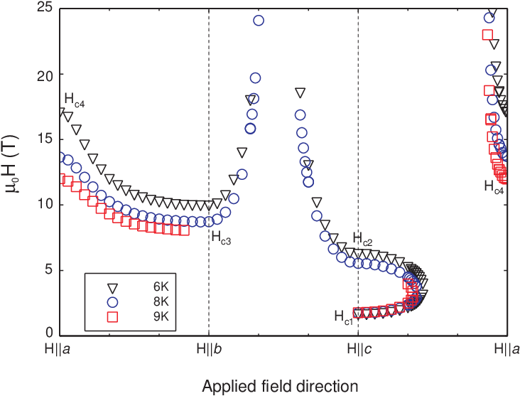
Finally, we also computed the angular dependence of the critical fields for spin-reorientation transitions (see Fig. 5). All the marked fields correspond to real transitions, accompanied by a jump in the susceptibility and by a sudden reorientation of the main order parameter $\mathbf{L}_{6}$. To ensure that the angular dependence is not affected by changes in magnitude of the main order parameter $\mathbf{L}_{6}$ (due to closeness to the PM-AFM phase boundary), the modelling was carried out at different temperatures (6, 8, and 9 K). All curves are qualitatively similar, with differences mostly due to the above mentioned temperature dependence of the upper critical fields $H_{c2,3,4}$ and, partially (for the 9 K curve), to the crossing of the PM-AFM phase boundary before a spin-reorientation transition has occurred. Our model predicts quite a remarkable angular dependence for the critical fields. On rotating from the hard axis $a$ towards the secondary easy-axis $b$, the critical field $H_{c4}$ transforms smoothly into $H_{c3}$. Upon further rotation towards the easy axis $c$, the field required for a spin-reorientation transition first grows very rapidly and, at an intermediate critical angle, diverges to infinity. Subsequently, it reappears from the high-field zone and finally converges to the critical field $H_{c2}$. A rotation from the easy axis $c$ towards the hard axis $a$ (right panel in Fig. 5) demonstrates the merging of the two critical fields $H_{c1}$ and $H_{c2}$ at a certain angle. Then the spin-reorientation transition reappears from high fields and, finally, close to the $a$ axis, evolves towards $H_{c4}$. To the best of our knowledge the angular dependence of the critical fields in BaCu₂Si₂O₇ has not yet been studied. Its experimental investigation would represent an independent additional test of the proposed model.

By making use of the Ginzburg-Landau theory of phase transitions we propose a semi-quantitative description of the magnetic phase diagram of 1D systems with competing interactions. We have demonstrated that the competition between the field-induced and the exchange-driven order parameters in a quasi-one-dimensional antiferromagnet can lead to an unusual phase diagram and to remarkable deviations of the magnetization process from that expected in a 1D Heisenberg antiferromagnet. Additionally, in the BaCu₂Si₂O₇ model system, we predict an unusual angular dependence of the critical fields, which will be object of future experimental investigations.