Vacuum structure and stability of a singlet fermion dark matter model with a singlet scalar messenger
Abstract
We consider the issue of vacuum stability and triviality bound of the singlet extension of the Standard Model (SM) with a singlet fermion dark matter (DM). In this model, the singlet scalar plays the role of a messenger between the SM sector and the dark matter sector. This model has two Higgs-like scalar bosons, and is consistent with all the data on electroweak precision tests, thermal relic density of DM and its direct detection constraints. We show that this model is stable without hitting Landau pole up to Planck scale for 125 GeV Higgs boson. We also perform a comprehensive study of vacuum structure, and point out that a region where electroweak vacuum is the global minimum is highly limited. In this model, both Higgs-like scalar bosons have reduced couplings to the SM weak gauge bosons and the SM fermions, because of the mixing between the SM Higgs boson and the singlet scalar. There is also a possibility of their invisible decay(s) into a pair of DM’s. Therefore this model would be disfavored if the future data on the or with and turn out larger than the SM predictions.
Keywords
vacuum structure, vacuum instability, singlet fermionic dark matter1 Introduction
The Standard Model (SM) has been extremely successful in describing interactions between quarks and leptons down to m, or up to a few TeV depending on the channels, and it would be complete if the Higgs sector is established experimentally, clarifying the origin of electroweak symmetry breaking (EWSB) and masses for the SM chiral fermions and EW gauge bosons.
However, the SM should be extended in order to accommodate 3 different directions:
- •
Neutrino masses and mixings cannot be explained within the context of renormalizable SM.
- •
Baryon number asymmetry of the universe requires a new source of CP violation, beyond the CKM phase in the SM [1].
- •
Nonbaryonic cold dark matter of the universe should be included in the SM.
Admittedly, the simplest and the most economic solution to the 1st and the 2nd problems is to invoke the seesaw mechanism [2] and leptogenesis by introducing extra singlet right-handed (RH) neutrinos [3]. This is also nicely fit to the idea of grand unified theory (GUT) based on and .
For the nonbaryonic cold dark matter, there are many candidates in particle physics models: axion and axino, the lightest supersymmetric particle (LSP) in SUSY models (neutralino or gravitino), the lightest Kaluza-Klein particle (LKP) in extra dimensional scenarios, to name only a few. Some of them are related with other problems in particle physics, such as strong CP problem or fine tuning problem of (Higgs mass)2, but there are many other models which are not related with other problems in particle physics.
Another possibility is to rely on the principle of Occam’s razor, namely the simplest extension of the SM with dark matter candidates. In terms of the least number of new degrees of freedom, a scalar DM model with symmetry would be the simplest one. However the origin of symmetry is not clear, since it is put in by hand. The simplest DM model without ad hoc symmetry would be a singlet Dirac fermion CDM with conserved charge associated with a global dark symmetry. In Ref. [4], three of the present authors proposed such a scenario, by considering a Dirac fermion DM () that couples to a real singlet scalar () (see also [5] and [6] for similar discussions). Writing the most general renormalizable lagrangian among these new fields ( and ) and the SM fields, including the so-called Higgs portal terms, we could describe the DM physics (thermal relic density and direct detection), and collider phenomenology and electroweak precision tests (EWPT). Adding the singlet scalar improves the overall EWPT fits [4].
In this model, the Higgs phenomenology is modified in an important way by two different reasons:
- •
There are two neutral Higgs-like scalar bosons, and , which are two mixtures of the SM Higgs boson and a singlet scalar , with a mixing angle . Couplings of and to the SM particles are reduced by or . Therefore the production cross sections for ’s at colliders will be reduced by or compared with that of the SM Higgs boson with the same mass.
- •
Both and can decay invisibly into a pair of DM if kinematically allowed : . This would make more difficult to observe the ’s produced at colliders.
These two independent mechanisms will make two Higgs-like scalar bosons have reduced signal strength into specific final states [ see Eq. (3.3) ].
Recently, ATLAS and CMS reported a tantalizing hint for a Higgs-like boson with mass around 125 GeV [7, 8, 9]. Its couplings to the , and are consistent with the SM predictions, albeit there are still large uncertainties because of limited statistics. More data accumulation is planned toward the end of this year, and we would learn much more about the detailed properties of the observed new Higgs-like boson.
If the SM Higgs boson has mass around 125 GeV, the electroweak (EW) vacuum might be meta-stable or even unstable due to the quantum corrections from top quark loop [10, 11, 12, 13, 14] though large uncertainties in determining SM quantities including top pole mass do not allow to draw a firm conclusion on this issue [13, 15, 16]. Meta-stability might be still allowed as long as the tunneling time to wrong vacuum is longer than the age of our universe. However, if the primordial inflation is supposed to take place along the direction of Higgs field, for example as the case of Higgs inflation [17], the possible meta-stability of EW vacuum should be improved [14] 11 1 Inflation due to Higgs field false vacuum [18, 19, 20] might be a possible alternative to Higgs inflation though the initial condition for inflation looks non-trivial to be realized. . Some new physics should be introduced well below the Planck scale in order to save this situation. It is the purpose of this paper to address this issue within the model proposed in Ref. [4]. In this model, there are only two more fields beyond the SM ones, the fermion DM and a real singlet scalar messenger . Since couples to the SM Higgs field directly, one can imagine that the EW vacuum in our model could be stable even if the new physics scale is as large as Planck scale. In other words, the Planck chimney could be possible for Higgs mass around 125 GeV.
However, once we introduce and into the SM, the vacuum structure can change significantly, which may give rise to various false vacua. For example, if develops the vacuum expectation value (VEV), the Higgs potential in the direction could take the form of a double-well potential. If it is tilted, it is no longer clear that the EW vacuum is the the global minimum. Furthermore, at the loop level contributes to the Higgs potential and may affect the vacuum structure as well. Nevertheless, such a vacuum analysis was often overlooked in the literature.
In this paper, we investigate the vacuum structure and stability in the SM with and . An effective potential approach is adopted to study the vacuum structure. We explore not only the EW vacuum but also other possible false vacua at the tree- and one-loop levels. At the tree level, we explicitly derive analytic expressions for the vacuum energies while the one-loop analysis exclusively relies on numerics.
In order to examine the vacuum instability occurring at the high-energy scale, we use the renormalization group (RG) method. The functions of all dimensionless couplings are derived at the one-loop level. As for the most relevant parameters such as the top quark Yukawa coupling, strong coupling and SU(2) doublet Higgs quartic coupling, we also include two-loop contributions coming from the SM sector. In addition to the vacuum stability, we also investigate the perturbativity of the quartic couplings up to the Planck scale.
This paper is organized as follows. In Sec. 2, we describe the model and the relevant constraints from colliders and dark matter physics are discussed in Sec. 3. In Sec. 4, we discuss the vacuum structures, and various vacua are scrutinized carefully. The stability of EW vacuum taking account of the RG effects up to some new physics scale is investigated in Sec. 5. The paper is summarized in Sec. 6. We collect the matching conditions used in our analysis in Appendix A, and the one-loop Higgs boson mass formulae as well as one-loop tadpole conditions are presented in Appendix B.
2 The model
We consider a SM gauge-singlet Dirac fermion DM () with a real singlet scalar () that couples to the SM sector by the Higgs portal [4]. The dark sector is described by the lagrangian
| (1) |
The most general renormalizable scalar potential including the Higgs portal interactions is given by
| (4) | |||||
where is the SM Higgs field.
In general, the neutral scalar fields develop nontrivial vacuum expectation values (VEVs), and . And we expand the neutral component of and as
in the unitary gauge. Then the minimization conditions of the Higgs potential at VEVs give
| (8) |
We introduce the Higgs mixing angle and the mass eigenvalues () which diagonalize the Higgs mass squared matrix such that
The quartic couplings, , in the Higgs potential can be expressed in terms of the Higgs mass parameters
| (18) |
so that they are obtained as a function of and which we take as input parameters. The mass eigenstates () with masses are written in terms of the SM Higgs scalar and the singlet scalar as
| (19) |
In the Higgs and dark sector we have 10 free parameters which are to be measured in the experiments:
| (20) |
The constraints on these parameters from perturbative unitarity of electroweak gauge boson scattering amplitudes, EWPT, collider searches for Higgs boson(s), DM relic density, DM direct detection experiments, were given in Ref. [4]. And those from the vacuum stability and triviality will be considered in this paper.
3 The constraints considered in Ref. [4]
In Ref. [4] we considered the following observables which can constrain our model:
The first three conditions do not constrain the dark matter sector, and they are also relevant to the singlet scalar extension of the SM without dark matter.
3.1 Perturbative unitarity of gauge boson scattering amplitudes
3.2 Collider bound
In Ref. [4] we defined two ratios () (what we called the reduction factor):
| (23) |
where is a specific SM final state, which measure the reduced signal strength with respect to the SM. In terms of the SM Higgs (singlet Higgs) decay width with mass , i.e. without the effect of the mixing, we get
| (24) |
We can see that the “reduction” of signal strength is a generic feature of this model, i.e. . If the future LHC data on for some (, ) is larger than 1, our model would be ruled out. In Ref. [4], we found that if , we get for (). So the heavy scalar boson will easily evade the detection at LHC.
If the Higgs splitting mode opens kinematically, it would provide a smoking gun signal for our model, like the four -jets, two-photons plus two -jets, four tau leptons, etc. The high-luminosity LHC machine can target these signals.
3.3 The oblique parameters:
In our model the new scalar particle can contribute to the and boson self-energy diagrams, , thereby changing the EWPT parameters [4]. Explicit expressions for the oblique parameters in our model can be found in Ref. [4]. The result is that including singlet scalar improves the overall fit to the EWPT, which can be seen in Fig. 1. For GeV, the mixing angle is constrained to be when GeV.

3.4 Dark matter relic density
The observed DM relic density, [26], is related with the thermally averaged annihilation cross section times relative velocity at freeze-out temperature roughly by22 2 There is a typo in this expression in Ref. [4] and we correct it here
| (25) |
The annihilation cross section of a DM pair is proportional to . Since the EWPT and LHC observation of the SM-like Higgs boson restricts to be small, the cross section is generically much smaller than is needed to explained the current relic density. This can be seen in Fig. 2 except for resonance regions.
At resonance, if , the non-relativistic approximation of the cross-section is [28]
| (26) |
where and . For example, ignoring decay, we find
| (27) |
If decays dominantly to dark matter,
| (28) | |||||
| (29) |
and hence
| (30) | |||||
| (31) |
where we have used and in the second line. Hence, even if might be constrained to be small, a right amount of CDM relic density can be obtained as long as is in the band of -channel resonance.
We used the micrOMEGAs package [29] for numerical calculation of DM relic density and direct detection cross section. In Fig. 2, we show the CDM relic density as a function of for various choices of GeV, with and . We can always find out the value which can accommodate thermal relic density of the singlet fermion CDM . Note that there is no strong constraint on the heavier Higgs with a small mixing angle , because would be mostly a singlet scalar so that it is very difficult to produce it at colliders, and also it could decay into a pair of CDM’s with a substantial branching ratio.

3.5 Direct detection
The null searches of the dark matter-proton scattering puts strong bounds on its spin-independent (SI) cross section [27]:
| (32) |
for the CDM in the mass range . The spin-dependent scattering cross section is zero in our model, because the scattering is due to two Higgs-like scalar bosons. Since the is proportional to the , the large annihilation cross section need for the relic density would also give large DM-proton scattering cross section, violating (32).
As pointed out in [4], there would be a destructive interference between and contributions to the scattering amplitude due to orthogonality of the Higgs mixing matrix, which is a very generic aspect in case there are extra singlet scalar bosons that can mix with the SM Higgs boson [30]. Hence, for regions , a cancellation occurs in and even the large , regions are only weakly constrained (see Fig. 4 of Ref. [4]). We also note that and are not strongly correlated near the Higgs resonance where the relic density can be explained. This helps to evade the strong bound on while accommodating the correct CDM density in the universe. This opens up a very interesting parameter space for Higgs boson search at the LHC, making one or two of the Higgs-like scalar bosons can decay into a pair of DM’s with a substantial invisible branching ratio(s).
3.6 Comparison with the effective lagrangian approach
In this subsection, we would like to compare our model with the so-called Higgs portal fermion dark matter model [31, 6], where the singlet scalar is presumed to be integrated out, resulting in the following model lagrangian:
| (33) |
Within this model, there is only one Higgs boson and its coupling to the DM is strongly constrained by the direct detection experiments. This result is very different from our analysis [4], where there is a generic cancellation between and contributions in the direct detection rates. In fact, depends also on , and it becomes zero when we ignore the mixing between the SM Higgs boson and the singlet scalar (see Eq. (3.16) of Ref. [4]). This result can never be obtained in the approach based on the above effective lagrangian (3.13). In our case the correlation between coupling and the direct detection cross section is not that strong compared with the results in Ref. [31]. It is important to consider the renormalizable models in order to discuss phenomenology related with the singlet fermion dark matter and Higgs bosons.
The same arguments also applies to the Higgs portal vector DM models, which is assumed to be described by the following lagrangian:
| (34) |
Although this lagrangian looks power-counting renormalizable, it is not really renormalizable. This is well known from the old intermediate vector boson theory for weak gauge boson . In order to give a mass to a spin-1 gauge boson, we need some symmetry breaking agency. Assuming a new complex scalar breaks the gauge symmetry spontaneously, one ends up with a new scalar boson from which would mix with the SM Higgs boson by Higgs portal. Therefore there will be two Higgs-like scalar boson in the end, and phenomenology in the scalar sector should be similar to that of the model described here and in Ref. [4]. We leave the detailed discussions of this issue for the future publication [30].
4 Vacuum structure
Because of the presence of the singlet scalar, the vacuum structure of this model is not that trivial. Since the Higgs potential is the quartic function of the Higgs fields (at the tree level), there could be another nondegenerate local minimum in the singlet Higgs direction unless some symmetry exists. If that is the case, our EW vacuum may not be global and its stability is unclear. In addition to this, the EW vacuum could be destabilized at a high energy scale by the RG effect of the top quark as in the SM. We separately examine the vacuum stability at the EW scale and the high energy scale. In this section, we focus on the former, and the latter will be discussed in the next section.
4.1 Tree level analysis
Let us first consider the vacuum structures of our model at tree level 33 3 The vacuum analysis of the singlet extension of the SM within the electroweak phase transition context can be found in [32]. . In this analysis, and are determined by Eq. (8) with fixed and . The tree-level effective potential then takes the form
| (35) |
where and are constant background fields. To avoid the potential unbounded from below, we impose
| (36) |
where the last condition is needed for .
Unlike the SM, there is a possibility that has a global minimum which is different from the prescribed vacuum . Following the Refs. [33, 34], we define the various vacua as follows:
| (37) | ||||
| (38) | ||||
| (39) | ||||
| (40) | ||||
| (41) |
where is the prescribed . In the phase III, although both and are nonzero, they are different from the prescribed vacuum (EW phase). Those various vacua are found by solving the following equations
| (42) | ||||
| (43) |
Note that one of the solutions corresponds to the EW phase. For the EW phase to be the global minimum, we require
| (44) |
where denote the VEVs in the SYM, I, II and III 44 4 Since we will not consider a case in which both and are simultaneously zero in the following discussion, the II phase would not be realized. . To begin with, we demonstrate a comparison between the EW and I phases. The vacuum energies of the both phases are as follows.
| (45) | ||||
| (46) |
Here, we define by taking the difference of the two vacuum energies
| (47) | |||||
To satisfy the condition (44), should be positive. However, it could be negative if gets large, which we will illustrate in the following. For simplicity we take . From Eq. (43), it follows that
| (48) |
where the second solution corresponds to the I phase, and should be satisfied for real solutions. The vacuum energy of the I phase is reduced to
| (49) |
Therefore, for the large values of and with their appropriate signs, we may have . As we will see later, the large can induce such a case.
Now we consider another solution in Eq. (42). The nonzero is expressed as
| (50) |
where the real solution of enforces . Plugging this into Eq. (43), we have a cubic equation for . If the cubic equation has only one real solution, it is nothing but and the III phase cannot exist. On the other hand, if the cubic equation has other real solutions, and simultaneously Eq. (50) has a real solution, the III phase would appear. In such a case, it should be checked whether the energy level of the EW vacuum is lower than that of the III phase. Let us denote the real solutions other than by and . We define as the solution that gives a local maximum and thus and its corresponding solution of yield the III phase.
Before going to the numerical analysis of the vacuum structures, we will obtain a range of consistent with the global vacuum conditions. To make the analysis simpler, we set . In the limit of , we may find
| (51) |
The vacuum energy of the EW phase then can be cast into the form
| (52) |
Requiring yields the lower bound of :
| (53) |
Furthermore, in the limit of , can be approximated as
| (54) |
Therefore, gives the upper bound of :
| (55) |
Similarly, we may also obtain another constraint on from . Instead of doing so, we investigate the vacuum structures numerically.


We begin with a case in which the EW vacuum becomes the local minimum and the III phase can be the global minimum. The representative example is shown in Fig. 3. We here take GeV, GeV, GeV, , . In the left panel, the red lines represent the prescribed VEVs (246 GeV, 500 GeV) and the upper and lower blue dotted curve denote and which significantly depend on the values of , and is mostly negative. In the right panel, the vacuum energies of the EW and III phases ( and) are shown, where is given by . We can see that holds only up to rad, and beyond this, the III phase becomes the global minimum.


As suggested by Eqs. (53) and (55), the region where the EW phase is the global minimum is also highly limited by the values of for a given and . In Fig. 4 we illustrate such constraints. In the upper panel, the vacuum structure is shown in the - plane, taking the same input parameters as those in Fig. 3. It is found that the EW phase can be the global minimum only for 160 GeV GeV, and in most of the parameter space, the III phase is the global minimum. It should be emphasized that the possible range of around rad is completely consistent with the analytic formulae and . From this observation, although we have not worked out the analytic formula from , the mass bounds on the second Higgs boson is more or less the same as and . In passing, we also find a region where the I phase becomes the global minimum at rad and GeV.
If the sign of is changed, namely, GeV is taken but keeping the rest of the input parameters, the vacuum structure is drastically changed as shown in the left lower panel. In this case, depending on and , the EW, SYM, I and III phases can become the global minimum. From this plot, we obtain the upper bound of the heavy Higgs boson mass, i.e., GeV around rad. Since is relatively large, this upper bound cannot be obtained from .
In the right panel, we set GeV. We can see that the global minimum region of the EW phases is significantly affected by the value of , rendering be as large as 800 GeV around rad. The possible lower value of is also pushed upward, GeV. For the small region, the allowed range of nicely agrees with the analytic formulae and .
4.2 One-loop level analysis
The tree-level Higgs potential receives the quantum corrections from the particles that couple to the Higgs fields. Therefore, the vacuum structure may change at the loop level. In our model, the DM in the hidden sector can also affect the Higgs potential through its couplings to the singlet Higgs field. So far, such an effect on the vacuum structure has not been investigated in the literature.
We analyze the vacuum structure using the one-loop effective potential [35]
| (56) |
which is regularized in the scheme; for scalars and fermions and for gauge bosons. is a renormalization scale which will be set on . is a field-dependent mass, and denotes particle species which is explicitly given by and their degrees of freedoms () are respectively given by
| (57) |
Unlike the tree-level analysis, it is impossible to obtain the analytic formulae of the vacuum structures. We thus numerically minimize
| (58) |
and find a global minimum. Since we are considering the vacuum stability at the low energy scale, we will concentrate on the fields space below 10 TeV.
We impose the one-loop tadpole conditions as
| (59) |
where , and is defined such that a field-dependent quantity is evaluated in the EW vacuum, namely, and . Since we are taking , , , and as the input parameters in place of , , , and , we solve the following coupled equations numerically
| (60) | ||||
| (61) | ||||
| (62) | ||||
| (63) |
where and are defined by the mass matrix of the Higgs bosons at the one-loop level. The explicit expressions of one-loop quantities are listed in Appendix B. Since the treatment of the Nambu-Goldstone (NG) boson loop contributions are somewhat tricky and numerically unimportant, we will not take them into account in the analysis here.


In Fig. 5, the vacuum structures at the one-loop level are shown. The input parameters in the Higgs sector are the same as in Fig. 4. As for the parameters in the DM sector, as an example, we set
| (64) |
In the upper plot, the significant difference between the tree and one-loop results is not observed in the entire region. As for the lower two plots, on the other hand, the region of the SYM phase appearing in the tree-level analysis vanishes, and the I phase region is enlarged instead. The reason is the following. At the tree level, solution can exist if as can be seen from Eqs. (42) and (43). At the one-loop level, on the contrary, there remain the constant terms in the tadpole condition for even after taking as we can observe in Eq. (112). Those constant terms are proportional to or which are always nonzero for the input parameters we are choosing here. Therefore, the SYM phase can never be realized at the one-loop level.
For GeV, the EW phase region is virtually unchanged and thus the allowed range of remains the same. For GeV, on the other hand, although the vacuum structure in the small region is not much affected by the one-loop contributions, the EW phase region is significantly distorted in , and the maximal can reach 1000 GeV around rad.
Here, we remark that since the chosen can be the half of in the allowed region, the DM relic density can be explained by the resonance effect as demonstrated in the previous section.


In order to see the DM loop effects on the vacuum structure, we vary as
| (65) |
taking and the rest of the parameters are the same as the previous cases. For the moment, we do not take account of the DM relic density constraint. Our findings are shown in Fig. 6. In the upper (lower) panels, GeV is taken, and in the left (right) panels, we set , where the red curves correspond to and the blue dotted curves represent . For the positive , the primary effect due to the increase of is the shift of the EW phase region to the right side, correspondingly, the minimal values of gets enhanced by about 25 (50) GeV around rad, and the maximal values of is enhanced by about 50 (200) GeV around rad in the case of GeV.
For the negative , on the other hand, the EW phase region is more sensitive to the change of , especially GeV case as shown in the upper right panel. The III phase region which can exist in the case is gone if , and the EW phase region is much enlarged. In this case, the range of GeV is allowed for any . The maximal value of , however, is reduced to 400 GeV which is realized at rad.
In the case of GeV, the minimal value of is increased by about 100 GeV, and the maximal value of it gets bigger by about 150 GeV when is changed from to .
Here, we comment on the DM relic density constraint. The choice of with Eq. (65) does not yield in the EW phase region. Therefore, the right amount of the DM relic density may not be guaranteed. It turns out that the change of has little effect on the vacuum structures once we take .
In summary, in this section we showed that the diverse types of the (false) vacua are realized in this model, which is due to the presence of the singlet scalar field. Most important consequence is that the EW vacuum is not always the global minimum and often becomes the metastable state. As explicitly demonstrated here, the global minimum condition for the EW vacuum can eliminate the large portion of the parameter space. As a result, we can obtain the strong bounds on . For rad, we find . Is should be stressed that this mass bound exclusively depends on and and not on the value of . For , however, the above range would not be valid any more. The EW phase regions appear somewhere near in which becomes the SM-like Higgs boson.
At the loop level, the DM also contributes to the effective potential. It is found that the vacuum structure has some sensitivity to the magnitude of , rendering the viable ranges of and changed. However, such effects would be diminished once is imposed, which is indeed the case if we wish to saturate the observed thermal relic density of CDM by a singlet fermion CDM.
5 Vacuum stability
Recent results of ATLAS and CMS experiments may indicate . If SM is assumed to be valid up to a very high energy scale, for example, GUT or Planck scale, the SM Higgs potential realizing such a light higgs faces the problem of vacuum instability, that is, the existence of non-SM deeper vacuum or unbound-from-below caused by the negativity of quartic self-coupling of Higgs at large field region. However, a simple extension of SM changes this situation drastically. As shown in the previous section, including a singlet which couples to SM via Higgs portal make vacuum structure very complicated. In this section, we show how the SM picture of instability problem of Higgs potential at high energy scale is changed in our model.
Before getting into the analysis, we fix the low energy boundary quantities at the scale of -boson pole mass.
| (66) |
where
| (67) |
We run up the couplings to the scale of top-quark running mass in -scheme. Denoted as , the running mass is obtained from the well-known formulas listed in Appendix. For the top-quark pole-mass [36]
| (68) |
we find
| (69) |
Correspondingly, the running top-Yukawa coupling is given by
| (70) |
Note that choosing as the matching scale results in which is smaller than by about . As shown in Fig. 7, this difference results in about higher instability scale of SM Higgs potential. It is similar size to the uncertainties of the top-quark pole mass and associated instability scale.

In order to obtain the running Higgs quartic coupling at , we solved Eqs. (60)-(63) numerically, ignoring momentum dependent corrections which is about %-level contributions [37] 55 5 In case of SM, a %-level correction to Higgs mass results in about an order of magnitude change of the instability scale. .
5.1 Tree-level (mixing) effect
The first thing we should note in a extension of SM like ours is how the mass of the SM-like higgs is determined. For the fixed VEV of SM Higgs field, is no more the only parameter which determines the mass of SM-like higgs. As studied in Refs. [38, 39], tree-level contribution of a singlet scalar can remove the instability problem in a very simple manner. Similarly, the tree-level effect of our model on the stability of SM Higgs potential can be read off from the mixing effect on the SM Higgs. At tree level, the SM Higgs quartic coupling can be written as
| (71) |
where is the mixing angle. If (no mixing), one obtains with . However, once the mixing is turned on, can be much larger than .
It may turn out that Higgs is very SM-like, so the mixing between the singlet and the SM Higgs might have to be highly suppressed. Even in such a case, we can still have a sizable increase of to achieve the stability of Higgs potential by pushing up to its unitary bound at most. If small, the mixing angle is given as
| (72) |
In the limit of large where the heavy singlet-like Higgs is likely to be decoupled, is approximated as
| (73) |
which is the same as the case of Ref. [39, 38]. On the other hand, if , the tree-level effect on is negligible, but the loop-effect from extra particles could be still large enough to remove the vacuum instability as long as is sizable.

In Fig. 8, we show contours in (,)-plane. If the RG-running of is pure SM-like, vacuum stability requires (corresponding to ) at 2-loop level. We can see in the figure that, even if , vacuum can be stable if .
5.2 Loop effect
5.2.1 RG equations
If is limited to be small due to constraints from collider experiments and/or direct searches of dark matter, we may have to resort to the additional loop contributions coming from the Yukawa couplings, , and .
The -function of a coupling in the renormalization group equation is defined as
| (74) |
where is the renormalization scale. For SM gauge couplings, the -functions are given as
| (75) |
where, for notational convenience, we have redefined the SM couplings as
| (76) |
and
| (77) | |||||
| (78) |
with
| (79) |
For dimensionless couplings (including the top Yukawa coupling) in the scalar potential, the 1-loop -functions are as follows.
| (80) | |||||
| (81) | |||||
| (82) | |||||
| (83) | |||||
| (84) |
For the top-Yukawa and quartic self couplings of Higgs field, the 2-loop -function contributions are as follows.
| (85) | |||||
| (86) | |||||
Note that is linearly proportional to , hence does not change its sign during its RG-running. does not change its sign, too, and it increases or decreases monotonically, depending its sign. appears in the RGEs of and as a squared one, so its sign does not affect RG-running of those couplings.
As can be seen from Eq. (84), the RGE of does not depend on any other couplings at 1-loop level. Hence it can be solved easily, giving the solution
| (87) |
We find that if
| (88) |
which corresponds to
| (89) |
where is the Planck mass. Note that has a strong dependence on , hence as becomes close to upper bound, the allowed band of for a perturbative positive becomes narrower and eventually disappears.
5.3 Numerical analysis
The aim of our numerical analysis is to see if the demand of vacuum stability constrains our model parameters which should satisfy EWPT, DM relic density and DM direction detection bound, and if there is any way to probe the model in future collider experiments. In this regard, the crucial parameters are
| (90) |
These parameters are involved in the following constraints.
- •
EWPT: , and
- •
DM relic density: The first 4 parameters
- •
DM direct searches: The first 4 parameters
- •
Vacuum stability ( and ): All of them.
Note that not all of those parameters are independent. For example, if we choose , and as an input, each element of the mass matrix is fixed through Eq. (2). Since , is fixed by the first line of Eq. (18), but we are free to choose and . Once () is chosen, () is given in terms of by the second and third lines of Eq. (18), respectively, where we assume . Therefore, the free parameters we can use in analyzing the scale dependence of dimensionless couplings are
| (91) |
Inspired by the recent results of LHC experiments, we take and vary and in the ranges,
| (92) |
Since we are interested in parameter space where couplings do not blow up, we consider ranging
| (93) |
We find that blows up if even for and . blows up if for and . If starts from a negative value, blows up if for and . Based on this observation, we scan the following ranges of our parameters.
| (94) |
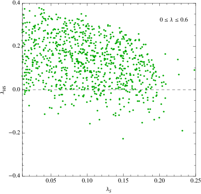
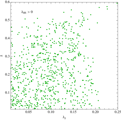
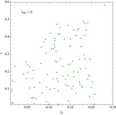
Fig. 9 shows a distribution of stable(red dots)/unstable(blue dots) vacua in (, ) plane for randomly chosen parameter sets. Left and right panels are for positive and negative , respectively. In both panels, the upper bound of red/blue dots are from the perturbativity constraints which we chose
| (95) |
In case of (left panel), red dots covers whole region below the perturbativity bound and go far below the SM bound. They appear even in the region where mixing is quite small. This is because non-zero can provide a large enough loop effect on the running of to remove the vacuum instability even if it is upper-bounded to a rather small value to avoid blow-up. On the other hand, for (right panel), quite small number of red dots(stable vacua) appear. This is because the constraint from unbounded-from-below at large field region removes big chunk of parameter space, which is clear from Fig. 10 and 11 where distributions of stable vacua shown in Fig. 9 are depicted in (,) and (,) planes, respectively.
As an example parameter set for stable vacuum, in Fig. 12 and 13, the RG-running of dimensionless couplings are shown for loop-effect only(left) and mixing only(right), respectively. Comparing both figures, we observe that, because of increasing magnitude of , the loop effect raises up the running of at high renormalization scale. Contrary to this, tree-level mixing effect is nearly like a simple shifting up of that can be also seen clearly in Fig. 14




The triviality and vacuum stability bound of Higgs mass as a function of the renormalization scale is shown in Fig. 14. Dashed lines in the figure corresponds to standard model bounds. Solid lines are bounds in our model. Note that in the left panel where only loop effect is included the solid-blue instability line is terminated at an intermediate scale of . It is because the quartic self-interaction of Higgs decreases at low scale but increases at high scale, as can be seen in the right panel of Fig. 12 66 6 As can be seen from Fig. 12, if is small, can cross-down zero-point at a scale, but cross-up at a higher scale. Instability, however, may not exist if SM-vacuum is the global minimum. Even if SM-vacuum is metastable, it is okay as long as the tunneling time is longer than the age of our universe. Cosmological danger of falling down to wrong vacuum may be also avoidable as long as Higgs field were in thermal touch with high temperature radiation background after inflation. . As shown in the figure, both of loop effect of and tree-level mixing can remove the vacuum instability easily in our model though they work differently.


5.4 Brief Summary
In brief summary, the numerical analysis shows that the vacuum stability of Higgs potential and perturbativity of couplings constrains new dimensionless couplings of our model as follows.
| (96) |
On the other hand, we cannot extract any useful bounds on the 2nd Higgs mass , since it depends on an unknown quantity, the singlet VEV .
6 Conclusion
In this paper, we have made a careful and comprehensive study of vacuum structure and vacuum stability in the singlet fermion dark matter with a real singlet scalar messenger. We found that the vacuum structure of this model has a very rich structure. In the parameter space we explore here, the EW, I, III and SYM phases (definitions are given in the text) appear, and any of them can become the global minimum. It is remarkable that the region where the EW vacuum is the global minimum is overly limited, eliminating the large parameter space. The tree-level analysis shows that the global vacuum condition yields the constraint on the mass of the second Higgs boson, i.e., for and 0.2 rad.
At the one-loop level, on top of the SM particles and singlet Higgs, the DM also participates in the effective potential. We found that effects of the DM on the vacuum structure can be significant depending on the magnitude and sign of . However, it tends to be small once we take which is favored by the DM relic abundance requirement. In such a case, above tree-level bound on is still valid at the one-loop level as verified numerically. Our findings also applies to the SM extension with a singlet scalar boson without CDM.
We also studied vacuum instability caused by the RG-running effect of the top quark at high-energy scales. Unlike the SM, in the current model can be positive all the way to the Planck scale. The reason is two-fold: due to the tree and loop effects coming from the singlet Higgs sector.
The former is related to the mixing between the doublet and singlet Higgs bosons at the tree level. Because of this, the Higgs quartic coupling and mass is no longer one-to-one correspondence. We can take larger with GeV by increasing and/or as shown in Eq. (71). This increment in the initial value of can avoid zero-crossing up to the Planck scale.
The latter is nothing but the effect of on the RG-running of . Such an effect can be sizable enough to compensate the negative contribution coming from the top quark at high-energy scale, preventing the Higgs potential from generating an unbounded-from-below direction or a potentially new global minimum. The perturbativity of the quartic couplings up to the Planck scale are also investigated. The results are summarized in Eq. (96).
Before closing, we make a comment on the bound of . Although we obtain the strong bound on through the global vacuum condition, is still not predictable since and are totally unknown. Therefore, we may need additional information to constrain those parameters somehow. For example, since strong first-order electroweak phase transition as needed for successful electroweak baryogenesis is closely related to specific vacuum structure and so the specific and , we may get more useful bound on . We leave this possibility to a future study.
7 Note Added
While we are finalizing this work, CMS and ATLAS Collaborations reported a new boson of mass around 125 GeV, which might be consistent with the SM Higgs boson. The invisible branching ratio of the observed particle seems to be small. In Fig. 15, we show the reduction factor for one of the Higgs boson mass is equal to 125 GeV. (Note that we took GeV in Ref. [4].)


Implications of this new results on the model studied in this work are the following:
- •
Since the observed properties of a new boson is close to those of the SM Higgs boson, its singlet component should be small, namely the mixing angle should be small in our model.
- •
If GeV, the singlet fermion DM mass may have to be greater than GeV so that is kinematically forbidden. The current Higgs search results can not be directly applied to , since would be mostly a singlet and difficult to be produced at colliders. Also it may decay into a pair of DM’s with a substantial branching ratio. Note that from Fig. 10 of Ref. [4].
- •
If GeV, the lighter Higgs boson can be light and may have escaped the detection if it is mostly SM singlet. This is still consistent with all the data available as of now.
- •
In order to test the idea of Higgs portal dark matter with a singlet fermion DM, it is important to search for two Higgs-like scalar bosons, one of which is to be identified with a new particle with mass around 125 GeV. The other scalar could be heavy and have escaped the Higgs search at the LHC and at the Tevatron, if it has substantial invisible branching ratio into a pair of DM’s.
- •
defined in Eq. (3.4) is always less than one in our model. Therefore, our model would be excluded, if turns out to be larger than one () in any of the decay channels in the future. On the other hand, if is observed in all observed channels in the future, our model could be a good candidate for the reason behind it. We have to wait for more precise determinations of for all possible measurable decay channels of Higgs-like boson with 125 GeV mass.
- •
In our model, there are two Higgs-like scalar bosons, one of which could be mostly singlet scalar and hard to discover at colliders, since . In Fig. 16, we show a scattered plot in the -plane for . Note that there is no strong constraint on the allowed mass range for the 2nd Higgs from the EWPT, collider or DM phenomenology. And the current SM Higgs search bounds do not apply directly, since the signal strength is reduced in our model () compared with the SM Higgs boson. Note that for all values of , for which case is always singlet-like. We find that for , making it difficult to search for the heavier (singlet-like) scalar particle. Therefore the current Higgs search should be continued for wider ranges of Higgs mass considering a possibility of , in order to look whether another Higgs-like scalar boson (mostly singlet-like) exists or not.
While we are finalizing this paper, there appeared a paper which considers Higgs phenomenology of a similar model, a singlet extension of the SM with DM in a hidden sector [40].
Acknowledgements
This work is supported in part by NRF Research Grant 2012R1A2A1A01006053 (PK and SB), and by SRC program of NRF Grant No. 20120001176 funded by MEST through Korea Nneutrino Research Center at Seoul National University (PK).
Appendix A The top-quark running mass
The top-quark pole-mass is related to the mass to NNLO as
| (97) |
where is the strong coupling with five active flavors, s are given as [41]
| (98) | |||||
| (99) | |||||
with and being zeta-constants. For matching, we have to set . At this scale the strong coupling can be found from the following relation for the running coupling
| (100) | |||||
where
| (101) | |||||
| (102) |
Appendix B Higgs boson masses at the one-loop level
Here, we write the useful formulae for the Higgs boson masses at the one-loop level. Let us begin by listing the field-dependent masses of all particles. The field-dependent masses of the Higgs bosons are given by the eigenvalues of the following 2-by-2 mass matrix
The field-dependent masses of the NG bosons, gauge bosons, top/bottom and singlet fermionic DM are respectively given by
| (107) | ||||
| (108) | ||||
| (109) | ||||
| (110) |
The one-loop tadpole conditions are cast into the form
| (111) | ||||
| (112) |
where
| (113) | ||||
| (114) | ||||
| (115) |
After imposing the one-loop tadpole conditions, the mass matrix elements of the Higgs bosons are
| (116) | ||||
| (117) | ||||
| (118) |
where
| (119) | ||||
| (120) | ||||
| (121) | ||||
| (122) | ||||
| (123) | ||||
| (124) | ||||
| (125) | ||||
| (126) | ||||
| (127) | ||||
| (128) |
References
- (1) M. B. Gavela, P. Hernandez, J. Orloff and O. Pene, Mod. Phys. Lett. A 9 (1994) 795 [hep-ph/9312215, hep-ph/9312215]; M. B. Gavela, P. Hernandez, J. Orloff, O. Pene and C. Quimbay, Nucl. Phys. B 430 (1994) 382 [hep-ph/9406289]; P. Huet and E. Sather, Phys. Rev. D 51 (1995) 379 [hep-ph/9404302]; T. Konstandin, T. Prokopec and M. G. Schmidt, Nucl. Phys. B 679 (2004) 246 [hep-ph/0309291].
- (2) P. Minkowski, Phys. Lett. B 67 (1977) 421; M. Gell-Mann, P. Ramond and R. Slansky, Conf. Proc. C 790927 (1979) 315; T. Yanagida, in Proceedings of the Workshop on Unified Theories and Baryon Number in the Universe, eds. O. Sawada and A. Sugamoto (KEK, Tsukuba, Japan, 1979); T. Yanagida, Prog. Theor. Phys. 64 (1980) 1103.
- (3) M. Fukugita and T. Yanagida, Phys. Lett. B 174 (1986) 45. For a review on leptogenesis, see W. Buchmuller and M. Plumacher, Int. J. Mod. Phys. A 15 (2000) 5047 [hep-ph/0007176]; W. Buchmuller, P. Di Bari and M. Plumacher, Annals Phys. 315 (2005) 305 [hep-ph/0401240]; W. Buchmuller, R. D. Peccei and T. Yanagida, Ann. Rev. Nucl. Part. Sci. 55 (2005) 311 [hep-ph/0502169]; M. -C. Chen, hep-ph/0703087 [HEP-PH]; S. Davidson, E. Nardi and Y. Nir, Phys. Rept. 466 (2008) 105 [arXiv:0802.2962 [hep-ph]].
- (4) S. Baek, P. Ko and W. -I. Park, JHEP 1202, 047 (2012) [arXiv:1112.1847 [hep-ph]].
- (5) Y. G. Kim, K. Y. Lee and S. Shin, JHEP 0805, 100 (2008) [arXiv:0803.2932 [hep-ph]].
- (6) L. Lopez-Honorez, T. Schwetz and J. Zupan, Phys. Lett. B 716 (2012) 179 [arXiv:1203.2064 [hep-ph]].
- (7) J. Incandela, CMS talk at Latest update in the search for the Higgs boson at CERN, July 4, 2012; F. Gianotti, ATLAS talk at Latest update in the search for the Higgs boson at CERN, July 4, 2012.
- (8) G. Aad et al. [The ATLAS Collaboration], arXiv:1207.7214 [hep-ex].
- (9) S. Chatrchyan et al. [The CMS Collaboration], arXiv:1207.7235 [hep-ex].
- (10) I. V. Krive and A. D. Linde, Nucl. Phys. B 117, 265 (1976).
- (11) N. Cabibbo, L. Maiani, G. Parisi and R. Petronzio, Nucl. Phys. B 158, 295 (1979).
- (12) G. W. Anderson, Phys. Lett. B 243, 265 (1990).
- (13) J. Elias-Miro, J. R. Espinosa, G. F. Giudice, G. Isidori, A. Riotto and A. Strumia, Phys. Lett. B 709, 222 (2012) [arXiv:1112.3022 [hep-ph]].
- (14) G. Degrassi, S. Di Vita, J. Elias-Miro, J. R. Espinosa, G. F. Giudice, G. Isidori and A. Strumia, JHEP 1208, 098 (2012) [arXiv:1205.6497 [hep-ph]].
- (15) S. Alekhin, A. Djouadi and S. Moch, arXiv:1207.0980 [hep-ph].
- (16) I. Masina, arXiv:1209.0393 [hep-ph].
- (17) F. L. Bezrukov and M. Shaposhnikov, Phys. Lett. B 659, 703 (2008) [arXiv:0710.3755 [hep-th]].
- (18) I. Masina and A. Notari, Phys. Rev. Lett. 108 (2012) 191302 [arXiv:1112.5430 [hep-ph]].
- (19) I. Masina and A. Notari, Phys. Rev. D 85 (2012) 123506 [arXiv:1112.2659 [hep-ph]].
- (20) I. Masina and A. Notari, arXiv:1204.4155 [hep-ph].
- (21) B. W. Lee, C. Quigg and H. B. Thacker, Phys. Rev. Lett. 38, 883 (1977).
- (22) C. Englert, T. Plehn, D. Zerwas, P. M. Zerwas, Phys. Lett. B703, 298-305 (2011). [arXiv:1106.3097 [hep-ph]].
- (23) R. Barate et al. [ LEP Working Group for Higgs boson searches and ALEPH and DELPHI and L3 and OPAL Collaborations ], Phys. Lett. B565, 61-75 (2003). [hep-ex/0306033].
- (24) M. E. Peskin and T. Takeuchi, Phys. Rev. Lett. 65, 964 (1990).
- (25) I. Maksymyk, C. P. Burgess and D. London, Phys. Rev. D 50, 529 (1994) [arXiv:hep-ph/9306267].
- (26) N. Jarosik, C. L. Bennett, J. Dunkley, B. Gold, M. R. Greason, M. Halpern, R. S. Hill, G. Hinshaw et al., Astrophys. J. Suppl. 192, 14 (2011). [arXiv:1001.4744 [astro-ph.CO]].
- (27) E. Aprile et al. [XENON100 Collaboration], arXiv:1207.5988 [astro-ph.CO].
- (28) P. Gondolo and G. Gelmini, Nucl. Phys. B 360, 145 (1991).
- (29) G. Belanger, F. Boudjema, A. Pukhov, A. Semenov, Comput. Phys. Commun. 180, 747-767 (2009). [arXiv:0803.2360 [hep-ph]].
- (30) S. Baek, P. Ko, W.I. Park and E. Senaha, work in preparation.
- (31) A. Djouadi, O. Lebedev, Y. Mambrini and J. Quevillon, Phys. Lett. B 709, 65 (2012) [arXiv:1112.3299 [hep-ph]].
- (32) J. R. Espinosa, T. Konstandin and F. Riva, Nucl. Phys. B 854 (2012) 592 [arXiv:1107.5441 [hep-ph]].
- (33) K. Funakubo, S. Tao and F. Toyoda, Prog. Theor. Phys. 114 (2005) 369 [hep-ph/0501052].
- (34) K. Cheung, T. -J. Hou, J. S. Lee and E. Senaha, Phys. Rev. D 82 (2010) 075007 [arXiv:1006.1458 [hep-ph]].
- (35) S. R. Coleman and E. J. Weinberg, Phys. Rev. D 7 (1973) 1888; R. Jackiw, Phys. Rev. D 9 (1974) 1686.
- (36) [Tevatron Electroweak Working Group and CDF and D0 Collaborations], arXiv:1107.5255 [hep-ex].
- (37) B. C. Allanach, A. Djouadi, J. L. Kneur, W. Porod and P. Slavich, JHEP 0409, 044 (2004) [hep-ph/0406166].
- (38) O. Lebedev, arXiv:1203.0156 [hep-ph].
- (39) J. Elias-Miro, J. R. Espinosa, G. F. Giudice, H. M. Lee and A. Strumia, JHEP 1206, 031 (2012) [arXiv:1203.0237 [hep-ph]].
- (40) B. Batell, D. McKeen and M. Pospelov, arXiv:1207.6252 [hep-ph].
- (41) U. Langenfeld, S. Moch and P. Uwer, Phys. Rev. D 80, 054009 (2009) [arXiv:0906.5273 [hep-ph]].