跳到论文正文
W Papers独立论文阅读器 arXiv:1209.4105 论文正文 计算阅读时间 · 0%
引用这篇论文根据当前论文元数据生成,正式投稿前建议核对。


License: arXiv.org perpetual non-exclusive license
arXiv:1209.4105v1 [hep-ph] 18 Sep 2012

KNO scaling from a nearly Gaussian action for small-xx gluons

Adrian Dumitrua,b,c and Elena Petreskab,c Affiliation: a RIKEN BNL Research Center, Brookhaven National Laboratory, Upton, NY 11973, USA
b Department of Natural Sciences, Baruch College, CUNY,
17 Lexington Avenue, New York, NY 10010, USA
c The Graduate School and University Center, The City University of New York, 365 Fifth Avenue, New York, NY 10016, USA
Abstract

Transverse momentum integrated multiplicities in the central region of p​ppp collisions at LHC energies satisfy Koba-Nielsen-Olesen scaling. We attempt to relate this finding to multiplicity distributions of soft gluons. KNO scaling emerges if the effective theory describing color charge fluctuations at a scale on the order of the saturation momentum is approximately Gaussian. From an evolution equation for quantum corrections which includes both saturation as well as fluctuations we find that evolution with the QCD β\beta-function satisfies KNO scaling while fixed-coupling evolution does not. Thus, non-linear saturation effects and running-coupling evolution are both required in order to reproduce geometric scaling of the DIS cross section and KNO scaling of virtual dipoles in a hadron wave function.

I Introduction

The color fields of hadrons boosted to the light cone are thought to grow very strong, parametrically of order A+∼1/gA^{+}\sim 1/g where gg is the coupling [1]. The fields of nuclei are enhanced further by the high density of valence charges per unit transverse area, which is proportional to the thickness A1/3A^{1/3} of a nucleus [2].

In collisions of such strong color fields a large number of soft gluons is released. Due to the genuinely non-perturbative dynamics of the strong color fields a semi-hard “saturation scale” QsQ_{s} emerges; it corresponds to the transverse momentum where the phase space density of produced gluons is of order 1/αs1/\alpha_{s}. The mean multiplicity per unit rapidity in high-energy collisions is then n¯≡⟨d​N/d​y⟩∼1/αs\bar{n}\equiv\langle dN/dy\rangle\sim 1/\alpha_{s}. Below we argue that a semi-classical effective theory of valence color charge fluctuations predicts that the variance of the multiplicity distribution is of order k−1∼𝒪⁡(αs0)k^{-1}\sim{\cal O}(\alpha_{s}^{0}) so that the perturbative expansion of n¯/k\bar{n}/k begins at order 1/αs≫11/\alpha_{s}\gg 1. We show that in the strong field limit then a Gaussian effective theory leads to Koba-Nielsen-Olesen (KNO) scaling [3]. This relates the emergence of KNO scaling in p⟂p_{\perp}-integrated multiplicity distributions from high-energy collisions to properties of soft gluons around the saturation scale.

Refer to caption
Figure 1: KNO scaling of charged particle multiplicity distributions in non-single diffractive p​p/p​p¯pp\,/\,p\overline{p} collisions at various energies as measured by the UA5 [4], ALICE [5] and CMS [6] collaborations, respectively. Note that we restrict to the bulk of the distributions up to 3.5 times the mean multiplicity.

The KNO scaling conjecture refers to the fact that the particle multiplicity distribution in high-energy hadronic collisions is universal (i.e., energy independent) if expressed in terms of the fractional multiplicity z≡n/n¯z\equiv n/\bar{n}. This is satisfied to a good approximation in the central (pseudo-) rapidity region at center of mass energies of 900 GeV and above [5, 6] as shown in fig. 1. On the other hand, UA5 data [4] taken at s=200\surd s=200 GeV appears to show a slightly distorted multiplicity distribution. This is in line with the observation that at lower energies higher-order factorial moments GqG_{q} of the distribution are energy dependent and significantly different from the reduced moments CqC_{q} [7]:

Gq≡⟨n(n−1)⋯(n−q+1)⟩n¯q,Cq≡⟨nq⟩n¯q.G_{q}\equiv\frac{\langle n\,(n-1)\cdots(n-q+1)\rangle}{\bar{n}^{q}}~~~,~~~C_{q}\equiv\frac{\langle n^{q}\rangle}{\bar{n}^{q}}~~. (1)

In fact, since the difference of GqG_{q} and CqC_{q} is subleading in the density of valence charges one may interpret this finding to indicate that the high density approximation is less accurate for s=200\surd s=200 GeV p​ppp collisions. Approximate KNO scaling has been predicted to persist also for min-bias p+P​bp+Pb collisions (at LHC energies) in spite of additional Glauber fluctuations of the number of participants and binary collisions [8]. A more detailed discussion of multiplicity distributions at TeV energies is given in refs. [9], and references therein.

Transverse momentum integrated multiplicities in inelastic hadronic collisions are not governed by an external hard scale, unlike say multiplicity distributions in e+​e−e^{+}e^{-} annihilation or in jets [10]. Hence, the explanation for the experimental observation should relate to properties of the distribution of produced gluons around the saturation scale QsQ_{s}.

II KNO scaling from a Gaussian action in the classical limit

We shall first discuss the multiplicity distribution of small-xx gluons obtained from a Gaussian effective action for the color charge fluctuations of the valence charge densities ρ\rho [2],

Z\displaystyle Z =\displaystyle= ∫𝒟​ρ​e−SM​V​[ρ],\displaystyle\int{\cal D}\rho\;e^{-S_{MV}[\rho]}~, (2)
SM​V​[ρ]\displaystyle S_{MV}[\rho] =\displaystyle= ∫d2​𝕩⟂​∫−∞∞d​x−​ρa​(x−,𝕩⟂)​ρa​(x−,𝕩⟂)2​μ2​(x−).\displaystyle\int d^{2}\mathbb{x}_{\perp}\int^{\infty}_{-\infty}dx^{-}~\frac{\rho^{a}(x^{-},\mathbb{x}_{\perp})\,\rho^{a}(x^{-},\mathbb{x}_{\perp})}{2\mu^{2}(x^{-})}~. (3)

In the strong field limit a semi-classical approximation is appropriate and the soft gluon field (in covariant gauge) can be obtained in the Weizsäcker-Williams approximation as

A+​(z−,𝕩⟂)=−g​1∇⟂2​ρa​(z−,𝕩⟂)=g​∫d2​𝕫⟂​∫d2​𝕜⟂(2​π)2​ei​𝕜⟂⋅(𝕩⟂−𝕫⟂)𝕜⟂2​ρa​(z−,𝕫⟂).A^{+}(z^{-},\mathbb{x}_{\perp})=-g\,\frac{1}{\nabla^{2}_{\perp}}\rho^{a}(z^{-},\mathbb{x}_{\perp})=g\int d^{2}\mathbb{z}_{\perp}\int\frac{d^{2}\mathbb{k}_{\perp}}{(2\pi)^{2}}\frac{e^{i\mathbb{k}_{\perp}\cdot(\mathbb{x}_{\perp}-\mathbb{z}_{\perp})}}{\mathbb{k}^{2}_{\perp}}\rho^{a}(z^{-},\mathbb{z}_{\perp})~. (4)

Parametrically, the mean multiplicity obtained from the action (3) is then

n¯∼Nc​(Nc2−1)αs​Qs2​S⟂,\bar{n}\sim\frac{N_{c}\,(N_{c}^{2}-1)}{\alpha_{s}}\;Q_{s}^{2}S_{\perp}~, (5)

where S⟂S_{\perp} denotes a transverse area and Qs∼g2​μQ_{s}\sim g^{2}\mu. The prefactor in (5) can be determined numerically [11, 12] but is not required for our present considerations.

One can similarly calculate the probability to produce qq particles by considering fully connected diagrams with qq valence sources ρ\rho in the amplitude and qq sources ρ∗\rho^{*} in the conjugate amplitude (for both projectile and target, respectively). These can be expressed as [13] 11 1 The rapidities y1⋯yqy_{1}\cdots y_{q} of the qq particles should be similar. Here we assume that all particles are in the same rapidity bin.

⟨dq​Ndy1⋯dyq⟩conn.=Cq⟨d​Nd​y1⟩⋯⟨d​Nd​yq⟩,\left<\frac{d^{q}N}{dy_{1}\cdots dy_{q}}\right>_{\rm conn.}=C_{q}\,\left<\frac{dN}{dy_{1}}\right>\cdots\left<\frac{dN}{dy_{q}}\right>~, (6)

where the reduced moments

Cq=(q−1)!kq−1.C_{q}=\frac{(q-1)!}{k^{q-1}}~. (7)

This expression is valid with logarithmic accuracy and was derived under the assumption that all transverse momentum integrals over pT,1⋯pT,qp_{T,1}\cdots p_{T,q} are effectively cut off in the infrared at a scale ∼Qs\sim Q_{s} due to non-linear effects.

The fluctuation parameter kk in eq. (7) is of order

k∼(Nc2−1)​Qs2​S⟂.k\sim(N_{c}^{2}-1)\,Q_{s}^{2}\,S_{\perp}~. (8)

Once again, the precise numerical prefactor (in the classical approximation) has been determined by a numerical computation to all orders in the valence charge density ρ\rho [15].

The multiplicity distribution is therefore a negative binomial distribution (NBD) [13],

P⁡(n)=Γ⁡(k+n)Γ⁡(k)​Γ​(n+1)​n¯n​kk(n¯+k)n+k.P(n)=\frac{\Gamma(k+n)}{\Gamma(k)\,\Gamma(n+1)}\frac{\bar{n}^{n}k^{k}}{(\bar{n}+k)^{n+k}}~. (9)

Indeed, multiplicity distributions observed in high-energy p​ppp collisions (in the central region) can be described quite well by a NBD, see for example refs. [8, 14]. The parameter k−1k^{-1} determines the variance of the distribution22 2 More precisely, the width is given by n¯​k−1+n¯−1∼n¯/k\bar{n}\,\sqrt{k^{-1}+\bar{n}^{-1}}\sim\bar{n}/\surd k; the latter approximation applies in the limit n¯/k≫1\bar{n}/k\gg 1, see below. and can be obtained from the (inclusive) double-gluon multiplicity:

⟨d2​Nd​y1​d​y2⟩conn.=1k​⟨d​Nd​y1⟩​⟨d​Nd​y2⟩.\left<\frac{d^{2}N}{dy_{1}dy_{2}}\right>_{\rm conn.}=\frac{1}{k}\;\left<\frac{dN}{dy_{1}}\right>\;\left<\frac{dN}{dy_{2}}\right>~. (10)

From this expression it is straightforward to see that the perturbative expansion of k−1k^{-1} starts at 𝒪⁡(αs0){\cal O}(\alpha_{s}^{0}) since the connected diagrams on the lhs of eq. (10) involve the same number of sources and vertices as the disconnected diagrams on the rhs of that equation (also see appendix). This observation is important since in general the NBD (9) exhibits KNO scaling only when n¯/k≫1\bar{n}/k\gg 1, and if kk is not strongly energy dependent. A numerical analysis of the multiplicity distribution at 2360 GeV, for example, achieves a good fit to the data for n¯/k≃6−7\bar{n}/k\simeq 6-7 [8], which we confirm below. Such values for n¯/k\bar{n}/k have also been found for peripheral collisions of heavy ions from ab initio solutions of the classical Yang-Mills equations [16]; furthermore those solutions predict that n¯/k<1\bar{n}/k<1 for central collisions of A∼200A\sim 200 nuclei.

To illustrate how deviations from KNO scaling arise it is instructive to consider a “deformed” theory with an additional contribution to the quadratic action. We shall add a quartic operator [17],

SQ​[ρ]=∫d2​𝕧⟂​∫−∞∞d​v1−​{ρa​(v1−,𝕧⟂)​ρa​(v1−,𝕧⟂)2​μ~2​(v1−)+∫−∞∞d​v2−​ρa​(v1−,𝕧⟂)​ρa​(v1−,𝕧⟂)​ρb​(v2−,𝕧⟂)​ρb​(v2−,𝕧⟂)κ4}.\displaystyle S_{Q}[\rho]=\int d^{2}\mathbb{v}_{\perp}\int^{\infty}_{-\infty}dv_{1}^{-}\left\{\frac{\rho^{a}(v_{1}^{-},\mathbb{v}_{\perp})\rho^{a}(v_{1}^{-},\mathbb{v}_{\perp})}{2\tilde{\mu}^{2}(v_{1}^{-})}+\int^{\infty}_{-\infty}dv_{2}^{-}\,\frac{\rho^{a}(v_{1}^{-},\mathbb{v}_{\perp})\rho^{a}(v_{1}^{-},\mathbb{v}_{\perp})\rho^{b}(v_{2}^{-},\mathbb{v}_{\perp})\rho^{b}(v_{2}^{-},\mathbb{v}_{\perp})}{\kappa_{4}}\right\}~. (11)

We assume that the contribution from the quartic operator is a small perturbation since κ4∼g​(g​A1/3)3\kappa_{4}\sim g\,(gA^{1/3})^{3} while μ~2∼g⁡(g​A1/3)\tilde{\mu}^{2}\sim g\,(gA^{1/3}). In the classical approximation the mean multiplicity is unaffected by the correction as it involves only two-point functions33 3 The two-point functions ⟨ρ​ρ⟩\langle\rho\rho\rangle in the theories (3) and (11) need to be matched. Thus, the “bare” parameters μ2\mu^{2} in (3) and μ~2\tilde{\mu}^{2} in (11) are different as the latter absorbs some self-energy corrections. We refer to ref. [17] for details.. On the other hand, k−1k^{-1} as defined in (10) now becomes

Nc2−12​π​Qs2​S⟂​1k\displaystyle\frac{N_{c}^{2}-1}{2\pi}Q_{s}^{2}\,S_{\perp}\frac{1}{k} =\displaystyle= 1−3​β​(Nc2+1)(with​β≡CF26​π3​g8Qs2​κ4​[∫−∞∞d​z−​μ4​(z−)]2).\displaystyle 1-3\beta\,(N_{c}^{2}+1)~~~~~~~~\left(\mathrm{with}~\beta\equiv\frac{C_{F}^{2}}{6\pi^{3}}\frac{g^{8}}{Q_{s}^{2}\,\kappa_{4}}\left[\int_{-\infty}^{\infty}dz^{-}\mu^{4}(z^{-})\right]^{2}\right)~. (12)
Refer to caption
Refer to caption
Figure 2: KNO scaling plots of charged particle multiplicity distributions at |η|<0.5|\eta|<0.5 in NSD collisions at various energies and NBD fits; z≡Nch/⟨Nch⟩z\equiv N_{\rm ch}/\langle N_{\rm ch}\rangle and Ψ⁡(z)≡⟨Nch⟩​P​(Nch)\Psi(z)\equiv\langle N_{\rm ch}\rangle\,P(N_{\rm ch}). Note that the mean multiplicity quoted for the fits has been rescaled by 1.5 to include neutral particles; also, that here kk is integrated over the transverse plane of the collision.

Therefore, in the classical approximation

n¯k∼Ncαs​(1−3​β​(Nc2+1)).\frac{\bar{n}}{k}\sim\frac{N_{c}}{\alpha_{s}}\left(1-3\beta\,(N_{c}^{2}+1)\right)~. (13)

This result illustrates that n¯/k\bar{n}/k decreases as the contribution of the ∼ρ4\sim\rho^{4} operator increases. We repeat that the derivation assumed that the correction is small so that (13) does not apply for large values of β​Nc2\beta N_{c}^{2}.

Ref. [17] estimated by entirely different considerations that for protons β≃0.01\beta\simeq 0.01 at x=10−2x=10^{-2}. That would correspond to a smaller value of n¯/k\bar{n}/k by a factor of 1.43 than for the Gaussian theory. Assuming that RG flow with energy approaches a Gaussian action [18], n¯/k\bar{n}/k should increase by about this factor. NBD fits to the data shown in fig. 2 confirm that n¯/k\bar{n}/k indeed increases with energy, which might indicate flow towards a Gaussian action; however, the observed increase from s=200\surd s=200 GeV to 7 TeV is much stronger: a factor of about 3. This apparent discrepancy could be resolved at least partially by running of the coupling in eqs. (5,13) with QsQ_{s} but this requires more careful analysis44 4 In fact, the running of αs\alpha_{s} at the effective scale QsQ_{s} is taken into account if the mean multiplicity is computed with energy evolved unintegrated gluon distributions like e.g. in refs. [8, 12]..

III Quantum evolution and the distribution of dipoles in the hadronic wave function

In the previous section we considered the multiplicity distribution of “produced gluons” in a collision of classical YM fields sourced by classical color charges ρ\rho moving on the light-cone. At high energies though (i.e., when αs​log⁡x−1∼1\alpha_{s}\log x^{-1}\sim 1) the classical fields are modified by quantum fluctuations [1]. Resummation of boost-invariant quantum fluctuations leads to an energy dependent saturation scale, for example, as required in order to reproduce the growth of the multiplicity n¯\bar{n} with energy. In particular, the energy dependence of the mean saturation scale, averaged over all “evolution ladders” (distribution of quantum emissions), can be obtained by solving the running-coupling BK equation [19].

Instead, in this section we shall solve a stochastic evolution equation which accounts both for saturation (non-linear) effects as well as for the fluctuations of the rapidities and transverse momenta of the virtual gluons in the wave function of a hadron before the collision. We do this in order to determine the multiplicity distribution (rather than just the mean number) of dipoles in a hadronic wave function boosted to rapidity YY.

We shall do so by solving via Monte-Carlo techniques the following evolution equation for P⁡[n⁡(x),Y]P[n(x),Y], which is the probability for the dipole size distribution n⁡(x)n(x) to occur:

∂P⁡[n⁡(x),Y]∂Y=∫zfz​[n⁡(x)−δx​z]​P​[n⁡(x)−δx​z,Y]−∫zfz​[n⁡(x)]​P​[n⁡(x),Y].\frac{\partial P[n(x),Y]}{\partial Y}=\int\limits_{z}f_{z}[n(x)-\delta_{xz}]\,P[n(x)-\delta_{xz},Y]-\int\limits_{z}f_{z}[n(x)]\,P[n(x),Y]~. (14)

Note that in this section x=log⁡ 1/r2x=\log\,1/r^{2} denotes the logarithmic dipole size (conjugate to its transverse momentum) rather than to a light-cone momentum fraction. This equation has been studied before in ref. [20] for fixed αs\alpha_{s} and in ref. [21] for running αs​(r2)\alpha_{s}(r^{2}). Those papers also provide references to related earlier work.

The first term in (14) is a gain term due to dipole splitting while the second term corresponds to loss due to “recombination”.

fz​[n⁡(x)]=Tz​[n​(x)]α⁡(z)f_{z}[n(x)]=\frac{T_{z}[n(x)]}{\alpha(z)} (15)

is the splitting rate and

Tz[n(x)]=1−exp∫xn(x)log(1−τ(z|x))T_{z}[n(x)]=1-\exp\int\limits_{x}n(x)\;\log\left(1-\tau(z|x)\right) (16)

is the dipole scattering amplitude for a dipole projectile of size zz to scatter off the target with the dipole distribution n⁡(x)n(x). Note that Tz​[n​(x)]T_{z}[n(x)] is non-linear in the dipole density as it involves also the pair (and higher) densities. Finally,

τ⁡(x|y)=α⁡(x)​α​(y)​exp⁡(−|x−y|)≡α⁡(r<2)​α​(r>2)​r<2r>2\tau(x|y)=\alpha(x)\alpha(y)\exp(-|x-y|)\equiv\alpha(r^{2}_{<})\,\alpha(r^{2}_{>})\,\frac{r^{2}_{<}}{r^{2}_{>}} (17)

is the elementary dipole-dipole scattering amplitude at LO in perturbative QCD. For more details we refer to ref. [21]. Here, we recall only that it was found there that evolution with a running coupling suppresses fluctuations in the tails of the travelling waves and so restores approximate geometric scaling [22].

We have determined the multiplicity distribution of dipoles with size ∼1/Qs​(Y)\sim 1/Q_{s}(Y),

Ni(Y)=∫r2<1/⟨Qs2​(Y)⟩dxni(x,Y)(i=1⋯105)N_{i}(Y)=\int\limits_{r^{2}<1/\langle Q_{s}^{2}(Y)\rangle}dx~n_{i}(x,Y)\hskip 56.9055pt(i=1\cdots 10^{5}) (18)

by evolving a given initial configuration n⁡(x,Y=0)n(x,Y=0) 10510^{5} times. Despite starting with a fixed initial condition, evolution introduces fluctuations in the rapidities where splittings occur, and in the sizes of the emerging dipoles.

Refer to caption
Refer to caption
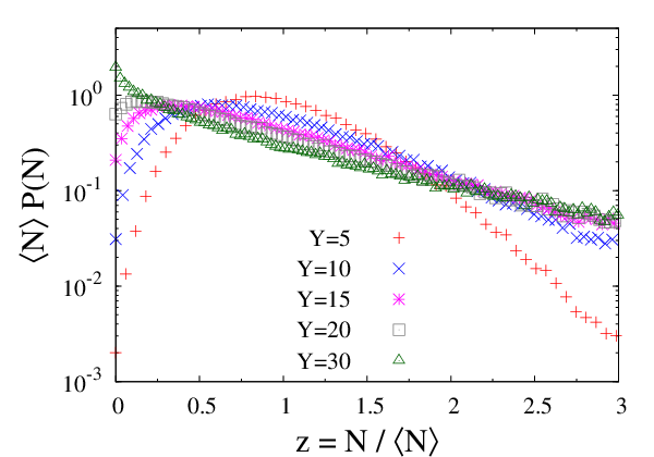
Figure 3: Multiplicity distribution of virtual dipoles with size r2<1/⟨Qs2​(Y)⟩r^{2}<1/\langle Q_{s}^{2}(Y)\rangle in the wave function. Left: evolution with trivial β\beta-function, αs=\alpha_{s}=const. Right: QCD β\beta-function.

In fig. 3 we show that fixed-coupling evolution does not obey KNO scaling of the distribution of virtual quanta while running-coupling evolution does. The shape of the distribution however looks different than the measured distribution of produced particles from fig. 1. This could be due to the fact that our evolution model does not treat diffusion in impact parameter space. Hence, P⁡(N)P(N) shown in fig. 3 should be interpreted as the multiplicity distribution at the center of the hadron.

Acknowledgements.
Our work is supported by the DOE Office of Nuclear Physics through Grant No. DE-FG02-09ER41620 and by The City University of New York through the PSC-CUNY Research Award Program, grant 65041-0043.

Appendix A The moment C2=k−1C_{2}=k^{-1} with the quartic action

We can obtain the fluctuation parameter kk by calculating the inclusive double gluon multiplicity and expressing it in terms of the single inclusive or mean multiplicity. The connected two particle production cross section for gluons with rapidity y1y_{1} and y2y_{2} has the form:

N2​(p,q)≡⟨d2​Nd​y1​d​y2⟩−⟨d​Nd​y1⟩​⟨d​Nd​y2⟩≡⟨d2​Nd​y1​d​y2⟩c​o​n​n.N_{2}(p,q)\equiv\left<\frac{d^{2}N}{dy_{1}dy_{2}}\right>-\left<\frac{dN}{dy_{1}}\right>\left<\frac{dN}{dy_{2}}\right>\equiv\left<\frac{d^{2}N}{dy_{1}dy_{2}}\right>_{conn.} (19)

⟨d​Nd​y⟩\left<\frac{dN}{dy}\right> is the mean multiplicity and the brackets denote an average over events. N2​(p,q)N_{2}(p,q) is given by:

N2(p,q)=g124​(2​π)6fg​a​a′fg′​b​b′fg​c​c′fg′​d​d′∫∏i=14d2​ki(2​π)2​ki2Lμ​(p,k1)​Lμ​(p,k2)​Lν​(q,k3)​Lν​(q,k4)(p−k1)2​(p−k2)2​(q−k3)2​(q−k4)2×\displaystyle N_{2}(p,q)=\frac{g^{12}}{4(2\pi)^{6}}f_{gaa^{\prime}}f_{g^{\prime}bb^{\prime}}f_{gcc^{\prime}}f_{g^{\prime}dd^{\prime}}\int\prod\limits_{i=1}^{4}\frac{d^{2}k_{i}}{(2\pi)^{2}k^{2}_{i}}\frac{L_{\mu}(p,k_{1})L^{\mu}(p,k_{2})L_{\nu}(q,k_{3})L^{\nu}(q,k_{4})}{(p-k_{1})^{2}(p-k_{2})^{2}(q-k_{3})^{2}(q-k_{4})^{2}}\times
⟨ρ1∗a​(k2)​ρ1∗b​(k4)​ρ1c​(k1)​ρ1d​(k3)⟩​⟨ρ2∗a′​(p−k2)​ρ2∗b′​(q−k4)​ρ2c′​(p−k1)​ρ2d′​(q−k3)⟩.\displaystyle\langle\rho_{1}^{*a}(k_{2})\rho_{1}^{*b}(k_{4})\rho_{1}^{c}(k_{1})\rho_{1}^{d}(k_{3})\rangle\langle\rho_{2}^{*a^{\prime}}(p-k_{2})\rho_{2}^{*b^{\prime}}(q-k_{4})\rho_{2}^{c^{\prime}}(p-k_{1})\rho_{2}^{d^{\prime}}(q-k_{3})\rangle~.~~~~~

LμL^{\mu} denotes the Lipatov vertex, for which:

Lμ​(p,k)​Lμ​(p,k)=−4​k2p2​(p−k)2.L_{\mu}(p,k)L^{\mu}(p,k)=-\frac{4k^{2}}{p^{2}}(p-k)^{2}~. (20)

For the four-point function in the target and projectile fields we use [17]

⟨ρ2∗a′​(p−k2)​ρ2∗b′​(q−k4)​ρ2c′​(p−k1)​ρ2d′​(q−k3)⟩=\displaystyle\langle\rho^{*a^{\prime}}_{2}(p-k_{2})\rho^{*b^{\prime}}_{2}(q-k_{4})\rho^{c^{\prime}}_{2}(p-k_{1})\rho^{d^{\prime}}_{2}(q-k_{3})\rangle=~~~~~~~~~~~~~~~~~~~~~~~~~~~~~~~~~~~~~~~~~~~~~
(2π)4[∫dz−μ~2(z−)]2[δa′​b′δc′​d′δ(p+q−k2−k4)δ(p+q−k1−k3)\displaystyle(2\pi)^{4}\,\left[\int dz^{-}\tilde{\mu}^{2}(z^{-})\right]^{2}\left[\delta^{a^{\prime}b^{\prime}}\delta^{c^{\prime}d^{\prime}}\delta(p+q-k_{2}-k_{4})\delta(p+q-k_{1}-k_{3})\right.~~~~~~~~~~~~
+δa′​c′δb′​d′δ(k1−k2)δ(k3−k4)+δa′​d′δb′​c′δ(p−q−k2+k3)δ(p−q−k1+k4)]\displaystyle\left.+\delta^{a^{\prime}c^{\prime}}\delta^{b^{\prime}d^{\prime}}\delta(k_{1}-k_{2})\delta(k_{3}-k_{4})+\delta^{a^{\prime}d^{\prime}}\delta^{b^{\prime}c^{\prime}}\delta(p-q-k_{2}+k_{3})\delta(p-q-k_{1}+k_{4})\right]
−(2​π)4​2π2​κ4​[∫d​z−​μ~4​(z−)]2​(δa′​b′​δc′​d′+δa′​c′​δb′​d′+δa′​d′​δb′​c′)​δ​(k1+k3−k2−k4).\displaystyle-(2\pi)^{4}\frac{2}{\pi^{2}\kappa_{4}}\left[\int dz^{-}\tilde{\mu}^{4}(z^{-})\right]^{2}\left(\delta^{a^{\prime}b^{\prime}}\delta^{c^{\prime}d^{\prime}}+\delta^{a^{\prime}c^{\prime}}\delta^{b^{\prime}d^{\prime}}+\delta^{a^{\prime}d^{\prime}}\delta^{b^{\prime}c^{\prime}}\right)\delta(k_{1}+k_{3}-k_{2}-k_{4})~.

The first two lines on the rhs of the above equation originate from the quadratic part of the action while the third line is due to the quartic operator. The product of the Gaussian parts of the two four-point functions gives nine terms, one of which (∼δa​c​δb​d​δa′​c′​δb′​d′)(\sim\delta^{ac}\delta^{bd}\delta^{a^{\prime}c^{\prime}}\delta^{b^{\prime}d^{\prime}}) corresponds to a disconnected contribution. It exactly cancels the second term in eq. (19).

Refer to caption
Figure 4: One of eight connected diagrams for two-gluon production with the quadratic MV action.

Four of the other eight terms (∼δa​c​δb​dCLOSE(\sim\delta^{ac}\delta^{bd} or OPEN∼δa′​c′​δb′​d′)\sim\delta^{a^{\prime}c^{\prime}}\delta^{b^{\prime}d^{\prime}}) give identical leading contributions to double gluon production. They correspond to a “rainbow” diagram like the one shown in Fig. 4. In the “rainbow” diagram, on one side (target or projectile), the ρ\rho’s corresponding to the same gluon momentum are contracted with each other. The remaining four “non-rainbow” diagrams are suppressed relative to the terms we keep at large pp and qq [13]. Hence, the leading Gaussian contribution is:

∼g128​π7​[∫d​z−​μ~2​(z−)]4​S⟂Qs2​Nc2​(Nc2−1)p4​q4.\sim\frac{g^{12}}{8\pi^{7}}\left[\int dz^{-}\tilde{\mu}^{2}(z^{-})\right]^{4}\frac{S_{\perp}}{Q_{s}^{2}}\frac{N_{c}^{2}(N_{c}^{2}-1)}{p^{4}q^{4}}~. (21)

The same reasoning applies also for the additional quartic contribution and only “rainbow” diagrams are considered, like the one in Fig. 5. There are two of them (one for the projectile and one for the target) to first order in κ4−1\kappa_{4}^{-1}, and their contribution is:

∼−g122​(2​π)6fg​a​a′fg′​b​b′fg​c​c′fg′​d​d′∫∏i=14d2​ki(2​π)2​ki2Lμ​(p,k1)​Lμ​(p,k2)​Lν​(q,k3)​Lν​(q,k4)(p−k1)2​(p−k2)2​(q−k3)2​(q−k4)2×\displaystyle\sim-\frac{g^{12}}{2(2\pi)^{6}}f_{gaa^{\prime}}f_{g^{\prime}bb^{\prime}}f_{gcc^{\prime}}f_{g^{\prime}dd^{\prime}}\int\prod\limits_{i=1}^{4}\frac{d^{2}k_{i}}{(2\pi)^{2}k^{2}_{i}}\frac{L_{\mu}(p,k_{1})L^{\mu}(p,k_{2})L_{\nu}(q,k_{3})L^{\nu}(q,k_{4})}{(p-k_{1})^{2}(p-k_{2})^{2}(q-k_{3})^{2}(q-k_{4})^{2}}\times
2​(2​π)8π2​κ4[∫dz−μ~2(z−)]2[∫dz−μ~4(z−)]2δa​cδb​dδ(k1−k2)δ(k3−k4)×\displaystyle\frac{2(2\pi)^{8}}{\pi^{2}\kappa_{4}}\left[\int dz^{-}\tilde{\mu}^{2}(z^{-})\right]^{2}\left[\int dz^{-}\tilde{\mu}^{4}(z^{-})\right]^{2}\delta^{ac}\delta^{bd}\delta(k_{1}-k_{2})\delta(k_{3}-k_{4})\times
(δa′​b′​δc′​d′+δa′​c′​δb′​d′+δa′​d′​δb′​c′)​δ​(k1+k3−k2−k4).\displaystyle\left(\delta^{a^{\prime}b^{\prime}}\delta^{c^{\prime}d^{\prime}}+\delta^{a^{\prime}c^{\prime}}\delta^{b^{\prime}d^{\prime}}+\delta^{a^{\prime}d^{\prime}}\delta^{b^{\prime}c^{\prime}}\right)\delta(k_{1}+k_{3}-k_{2}-k_{4})~.
Refer to caption
Figure 5: Connected diagram for two-gluon production from the quartic operator in the action [17].

The color factor evaluates to

fg​a​a′​fg′​b​b′​fg​c​c′​fg′​d​d′​δa​c​δb​d​(δa′​b′​δc′​d′+δa′​c′​δb′​d′+δa′​d′​δb′​c′)=2​Nc2​(Nc2−1)+Nc2​(Nc2−1)2.f_{gaa^{\prime}}f_{g^{\prime}bb^{\prime}}f_{gcc^{\prime}}f_{g^{\prime}dd^{\prime}}\delta^{ac}\delta^{bd}\left(\delta^{a^{\prime}b^{\prime}}\delta^{c^{\prime}d^{\prime}}+\delta^{a^{\prime}c^{\prime}}\delta^{b^{\prime}d^{\prime}}+\delta^{a^{\prime}d^{\prime}}\delta^{b^{\prime}c^{\prime}}\right)=2N_{c}^{2}(N_{c}^{2}-1)+N_{c}^{2}(N_{c}^{2}-1)^{2}~.

Using eq. (20) we get:

−16​g12(2​π)8​π2​κ4[∫dz−μ~2(z−)]2[∫dz−μ~4(z−)]2[2Nc2(Nc2−1)+Nc2(Nc2−1)2]×\displaystyle-\frac{16g^{12}}{(2\pi)^{8}\pi^{2}\kappa_{4}}\left[\int dz^{-}\tilde{\mu}^{2}(z^{-})\right]^{2}\left[\int dz^{-}\tilde{\mu}^{4}(z^{-})\right]^{2}\left[2N_{c}^{2}(N_{c}^{2}-1)+N_{c}^{2}(N_{c}^{2}-1)^{2}\right]\times
S⟂p2​q2​∫d2​k1k12​(p−k1)2​∫d2​k3k32​(q−k3)2.\displaystyle\frac{S_{\perp}}{p^{2}q^{2}}\int\frac{d^{2}k_{1}}{k_{1}^{2}(p-k_{1})^{2}}\int\frac{d^{2}k_{3}}{k_{3}^{2}(q-k_{3})^{2}}~.

The integral over the ladder momentum is again cut off at the saturation scale QsQ_{s}:

∫d2​k1k12​(p−k1)2≈2​πp2​log⁡pQs.\int\frac{d^{2}k_{1}}{k_{1}^{2}(p-k_{1})^{2}}\approx\frac{2\pi}{p^{2}}\log\frac{p}{Q_{s}}~.

Then, the quartic contribution to connected two gluon production becomes

−g124​π8​κ4​[∫d​z−​μ~2​(z−)]2​[∫d​z−​μ~4​(z−)]2​[2​Nc2​(Nc2−1)+Nc2​(Nc2−1)2]​S⟂p4​q4​log⁡pQs​log​qQs.-\frac{g^{12}}{4\pi^{8}\kappa_{4}}\left[\int dz^{-}\tilde{\mu}^{2}(z^{-})\right]^{2}\left[\int dz^{-}\tilde{\mu}^{4}(z^{-})\right]^{2}\left[2N_{c}^{2}(N_{c}^{2}-1)+N_{c}^{2}(N_{c}^{2}-1)^{2}\right]\frac{S_{\perp}}{p^{4}q^{4}}\log\frac{p}{Q_{s}}\log\frac{q}{Q_{s}}~. (22)

The last step is to express the fully connected diagrams in terms of the single inclusive cross section:

⟨d​Nd​y⟩=g64​π4​[∫d​z−​μ~2​(z−)]2​Nc​(Nc2−1)​S⟂p4​log⁡pQs.\left<\frac{dN}{dy}\right>=\frac{g^{6}}{4\pi^{4}}\left[\int dz^{-}\tilde{\mu}^{2}(z^{-})\right]^{2}N_{c}(N_{c}^{2}-1)\frac{S_{\perp}}{p^{4}}\log\frac{p}{Q_{s}}~. (23)

Summing eq. (21) and eq. (22) and using eq. (23) we get:

⟨d2​Nd​y1​d​y2⟩c​o​n​n.=[2​πQs2​(Nc2−1)​S⟂−4​(Nc2+1)κ4​S⟂​(Nc2−1)​[∫d​z−​μ~4​(z−)]2[∫d​z−​μ~2​(z−)]2]​⟨d​Nd​y1⟩​⟨d​Nd​y2⟩.\left<\frac{d^{2}N}{dy_{1}dy_{2}}\right>_{conn.}=\left[\frac{2\pi}{Q_{s}^{2}(N_{c}^{2}-1)S_{\perp}}-\frac{4(N_{c}^{2}+1)}{\kappa_{4}S_{\perp}(N_{c}^{2}-1)}\frac{\left[\int dz^{-}\tilde{\mu}^{4}(z^{-})\right]^{2}}{\left[\int dz^{-}\tilde{\mu}^{2}(z^{-})\right]^{2}}\right]\left<\frac{dN}{dy_{1}}\right>\left<\frac{dN}{dy_{2}}\right>~.

The fluctuation parameter k−1k^{-1} is now identified with the expression in the square brackets. We rewrite it in terms of

β≡CF26​π3​g8Qs2​κ4​[∫d​z−​μ~4​(z−)]2,\beta\equiv\frac{C_{F}^{2}}{6\pi^{3}}\frac{g^{8}}{Q_{s}^{2}\kappa_{4}}\left[\int dz^{-}\tilde{\mu}^{4}(z^{-})\right]^{2}~, (24)

and use

Qs2=g4​CF2​π​∫d​z−​μ~2​(z−),Q_{s}^{2}=\frac{g^{4}C_{F}}{2\pi}\int dz^{-}\tilde{\mu}^{2}(z^{-})~, (25)

to arrive at the final expression

Nc2−12​π​Qs2​S⟂​1k=1−3​β​(Nc2+1).\frac{N_{c}^{2}-1}{2\pi}\,Q_{s}^{2}S_{\perp}\,\frac{1}{k}=1-3\beta(N_{c}^{2}+1)~. (26)

Appendix B The moment C3C_{3} with the quartic action

In this section we are going to calculate the connected diagrams for three-gluon production to obtain the correction to the reduced moment C3C_{3} at order 1/κ4∼1/[g​(g​A1/3)3]1/\kappa_{4}\sim 1/[g(gA^{1/3})^{3}], assuming as before that g​A1/3>1gA^{1/3}>1. At the end of this section we also outline corrections suppressed by higher powers of g​A1/3gA^{1/3}.

We are looking for the contribution of the connected diagrams to the following expression [23]:

⟨d3​Nd​y1​d​y2​d​y3⟩=(−i​g3)68​(2​π)9fg​a​a′fg′​b​b′fg′′​c​c′fg​f​f′fg′​e​e′fg′′​d​d′×\displaystyle\left<\frac{d^{3}N}{dy_{1}dy_{2}dy_{3}}\right>=\frac{(-ig^{3})^{6}}{8(2\pi)^{9}}f_{gaa^{\prime}}f_{g^{\prime}bb^{\prime}}f_{g^{\prime\prime}cc^{\prime}}f_{gff^{\prime}}f_{g^{\prime}ee^{\prime}}f_{g^{\prime\prime}dd^{\prime}}\times~~~~~~~~~~~~~~~~~~~~~~~~~~~~~~~~~~~
∫∏i=16d2​ki(2​π)2​ki2Lα​(p,k1)​Lα​(p,k2)​Lβ​(q,k3)​Lβ​(q,k4)​Lγ​(l,k5)​Lγ​(l,k6)(p−k1)2​(p−k2)2​(q−k3)2​(q−k4)2​(l−k5)2​(l−k6)2×\displaystyle\int\prod\limits_{i=1}^{6}\frac{d^{2}k_{i}}{(2\pi)^{2}k^{2}_{i}}\frac{L_{\alpha}(p,k_{1})L^{\alpha}(p,k_{2})L_{\beta}(q,k_{3})L^{\beta}(q,k_{4})L_{\gamma}(l,k_{5})L^{\gamma}(l,k_{6})}{(p-k_{1})^{2}(p-k_{2})^{2}(q-k_{3})^{2}(q-k_{4})^{2}(l-k_{5})^{2}(l-k_{6})^{2}}\times
⟨ρ1∗f(p−k2)ρ1∗e(q−k4)ρ1∗d(l−k6)ρ1a(p−k1)ρ1b(q−k3)ρ1c(l−k5)⟩×\displaystyle\langle\rho_{1}^{*f}(p-k_{2})\rho_{1}^{*e}(q-k_{4})\rho_{1}^{*d}(l-k_{6})\rho_{1}^{a}(p-k_{1})\rho_{1}^{b}(q-k_{3})\rho_{1}^{c}(l-k_{5})\rangle\times
⟨ρ2∗f′​(k2)​ρ2∗e′​(k4)​ρ2∗d′​(k6)​ρ2a′​(k1)​ρ2b′​(k3)​ρ2c′​(k5)⟩.\displaystyle\langle\rho_{2}^{*f^{\prime}}(k_{2})\rho_{2}^{*e^{\prime}}(k_{4})\rho_{2}^{*d^{\prime}}(k_{6})\rho_{2}^{a^{\prime}}(k_{1})\rho_{2}^{b^{\prime}}(k_{3})\rho_{2}^{c^{\prime}}(k_{5})\rangle~.~~~~~~~~~~~~~~~~~~~~~~~~~~~~~ (27)

As before, the ρ\rho correlators of the target and the projectile consist of two parts, one from the quadratic operator in the action and another from the additional ρ4\rho^{4} operator:

⟨ρ∗f​ρ∗e​ρ∗d​ρa​ρb​ρc⟩=⟨ρ∗f​ρ∗e​ρ∗d​ρa​ρb​ρc⟩Gaussian+⟨ρ∗f​ρ∗e​ρ∗d​ρa​ρb​ρc⟩Correction.\langle\rho^{*f}\rho^{*e}\rho^{*d}\rho^{a}\rho^{b}\rho^{c}\rangle=\langle\rho^{*f}\rho^{*e}\rho^{*d}\rho^{a}\rho^{b}\rho^{c}\rangle_{\text{Gaussian}}+\langle\rho^{*f}\rho^{*e}\rho^{*d}\rho^{a}\rho^{b}\rho^{c}\rangle_{\text{Correction}}~.

The product of the two Gaussian contributions from the target and the projectile, to leading order in the gluon momenta, gives rise to 16 ”rainbow” diagrams. The result has been obtained previously [13] and reads (expressed in terms of the mean multiplicity):

⟨d3​Nd​y1​d​y2​d​y3⟩Conn. Gaussian=8​π2Qs4​S⟂2​(Nc2−1)2​⟨d​Nd​y1⟩​⟨d​Nd​y2⟩​⟨d​Nd​y3⟩.\left<\frac{d^{3}N}{dy_{1}dy_{2}dy_{3}}\right>_{\text{Conn. Gaussian}}=\frac{8\pi^{2}}{Q_{s}^{4}S_{\perp}^{2}(N_{c}^{2}-1)^{2}}\left<\frac{dN}{dy_{1}}\right>\left<\frac{dN}{dy_{2}}\right>\left<\frac{dN}{dy_{3}}\right>~. (28)

The correction, to first order in κ4−1\kappa_{4}^{-1} is

∼2​⟨ρ∗f′​ρ∗e′​ρ∗d′​ρa′​ρb′​ρc′⟩Gaussian​⟨ρ∗f​ρ∗e​ρ∗d​ρa​ρb​ρc⟩Correction.\sim 2\langle\rho^{*f^{\prime}}\rho^{*e^{\prime}}\rho^{*d^{\prime}}\rho^{a^{\prime}}\rho^{b^{\prime}}\rho^{c^{\prime}}\rangle_{\text{Gaussian}}~\langle\rho^{*f}\rho^{*e}\rho^{*d}\rho^{a}\rho^{b}\rho^{c}\rangle_{\text{Correction}}~. (29)

Again, we are considering only rainbow diagrams, so for the Gaussian six-point function in the above expression, from all possible contractions, we keep only the term

(2​π)6​[∫d​z−​μ~2​(z−)]3​δa′​f′​δb′​e′​δc′​d′​δ​(k1−k2)​δ​(k3−k4)​δ​(k5−k6).(2\pi)^{6}\left[\int dz^{-}\tilde{\mu}^{2}(z^{-})\right]^{3}\delta^{a^{\prime}f^{\prime}}\delta^{b^{\prime}e^{\prime}}\delta^{c^{\prime}d^{\prime}}\delta(k_{1}-k_{2})\delta(k_{3}-k_{4})\delta(k_{5}-k_{6})~.

To calculate the correction to the six-point function to first order in κ4−1\kappa_{4}^{-1} we factorize it into a product of two- and four-point functions. There are fifteen possible factorizations of that kind. Three of them are disconnected diagrams and the remaining twelve give identical contributions. We consider, for example, the following combination:

⟨ρ1∗f​(p−k2)​ρ1∗e​(q−k4)​ρ1∗d​(l−k6)​ρ1a​(p−k1)​ρ1b​(q−k3)​ρ1c​(l−k5)⟩\displaystyle\langle\rho_{1}^{*f}(p-k_{2})\rho_{1}^{*e}(q-k_{4})\rho_{1}^{*d}(l-k_{6})\rho_{1}^{a}(p-k_{1})\rho_{1}^{b}(q-k_{3})\rho_{1}^{c}(l-k_{5})\rangle~~~~~~~~~~~~~~~~~~~~~~~~~~~~~~~~~~
=⟨ρ1a​(p−k1)​ρ1b​(q−k3)⟩​⟨ρ1∗f​(p−k2)​ρ1∗e​(q−k4)​ρ1∗d​(l−k6)​ρ1c​(l−k5)⟩.\displaystyle=\langle\rho_{1}^{a}(p-k_{1})\rho_{1}^{b}(q-k_{3})\rangle\langle\rho_{1}^{*f}(p-k_{2})\rho_{1}^{*e}(q-k_{4})\rho_{1}^{*d}(l-k_{6})\rho_{1}^{c}(l-k_{5})\rangle~.~~~~~~~~~~~~~~~~~~~~~

The two point function is

⟨ρ1a​(p−k1)​ρ1b​(q−k3)⟩=(2​π)2​[∫d​z−​μ~2​(z−)]​δa​b​δ​(p+q−k1−k3),\langle\rho_{1}^{a}(p-k_{1})\rho_{1}^{b}(q-k_{3})\rangle=(2\pi)^{2}\left[\int dz^{-}\tilde{\mu}^{2}(z^{-})\right]\delta^{ab}\delta(p+q-k_{1}-k_{3})~,

and for the correction to the four-point function we use the last line from eq. (A).

The color factor is

fg​a​a′​fg′​b​b′​fg′′​c​c′​fg​f​f′​fg′​e​e′​fg′′​d​d′​δa​b​(δc​d​δe​f+δc​e​δd​f+δc​f​δd​e)​δa′​f′​δb′​e′​δc′​d′\displaystyle f_{gaa^{\prime}}f_{g^{\prime}bb^{\prime}}f_{g^{\prime\prime}cc^{\prime}}f_{gff^{\prime}}f_{g^{\prime}ee^{\prime}}f_{g^{\prime\prime}dd^{\prime}}\delta^{ab}\left(\delta^{cd}\delta^{ef}+\delta^{ce}\delta^{df}+\delta^{cf}\delta^{de}\right)\delta^{a^{\prime}f^{\prime}}\delta^{b^{\prime}e^{\prime}}\delta^{c^{\prime}d^{\prime}}
=2​Nc3​(Nc2−1)+Nc3​(Nc2−1)2.\displaystyle=2N_{c}^{3}(N_{c}^{2}-1)+N_{c}^{3}(N_{c}^{2}-1)^{2}~.~~~~~~~~~~~~~~~~~~~~~~~~~~~~

Putting everything together into eq. (27) and multiplying by two [because of (29)] and by twelve (which is the number of possible diagrams) we get:

⟨d3​Nd​y1​d​y2​d​y3⟩Conn. Correction=48​g18​πκ4[∫dz−μ~2(z−)]4[∫dz−μ~4(z−)]2[2Nc3(Nc2−1)+Nc3(Nc2−1)2]×\displaystyle\left<\frac{d^{3}N}{dy_{1}dy_{2}dy_{3}}\right>_{\text{Conn. Correction}}=\frac{48g^{18}\pi}{\kappa_{4}}\left[\int dz^{-}\tilde{\mu}^{2}(z^{-})\right]^{4}\left[\int dz^{-}\tilde{\mu}^{4}(z^{-})\right]^{2}\left[2N_{c}^{3}(N_{c}^{2}-1)+N_{c}^{3}(N_{c}^{2}-1)^{2}\right]\times
∫∏i=16d2​ki(2​π)2​ki2Lα​(p,k1)​Lα​(p,k2)​Lβ​(q,k3)​Lβ​(q,k4)​Lγ​(l,k5)​Lγ​(l,k6)(p−k1)2​(p−k2)2​(q−k3)2​(q−k4)2​(l−k5)2​(l−k6)2×\displaystyle\int\prod\limits_{i=1}^{6}\frac{d^{2}k_{i}}{(2\pi)^{2}k^{2}_{i}}\frac{L_{\alpha}(p,k_{1})L^{\alpha}(p,k_{2})L_{\beta}(q,k_{3})L^{\beta}(q,k_{4})L_{\gamma}(l,k_{5})L^{\gamma}(l,k_{6})}{(p-k_{1})^{2}(p-k_{2})^{2}(q-k_{3})^{2}(q-k_{4})^{2}(l-k_{5})^{2}(l-k_{6})^{2}}\times~~~~~~~~
δ⁡(k1−k2)​δ​(k3−k4)​δ​(k5−k6)​δ​(p+q−k1−k3)​δ​(p+q−k2−k4−k6+k5)\displaystyle\delta(k_{1}-k_{2})\delta(k_{3}-k_{4})\delta(k_{5}-k_{6})\delta(p+q-k_{1}-k_{3})\delta(p+q-k_{2}-k_{4}-k_{6}+k_{5})
=−3​g1816​κ4​π13S⟂p2​q2​l2[∫dz−μ~2(z−)]4[∫dz−μ~4(z−)]2[2Nc3(Nc2−1)+Nc3(Nc2−1)2]×\displaystyle=-\frac{3g^{18}}{16\kappa_{4}\pi^{13}}\frac{S_{\perp}}{p^{2}q^{2}l^{2}}\left[\int dz^{-}\tilde{\mu}^{2}(z^{-})\right]^{4}\left[\int dz^{-}\tilde{\mu}^{4}(z^{-})\right]^{2}\left[2N_{c}^{3}(N_{c}^{2}-1)+N_{c}^{3}(N_{c}^{2}-1)^{2}\right]\times
∫d2​k1k12​(p+q−k1)2​(p−k1)4​∫d2​k2k22​(l−k2)2.\displaystyle\int\frac{d^{2}k_{1}}{k_{1}^{2}(p+q-k_{1})^{2}(p-k_{1})^{4}}\int\frac{d^{2}k_{2}}{k_{2}^{2}(l-k_{2})^{2}}~.

Again, we regularize the ladder integrals at the saturation scale,

∫d2​kk2​(p+q−k)2​(p−k)4≃2​πp2​q2​1Qs2.\int\frac{d^{2}k}{k^{2}(p+q-k)^{2}(p-k)^{4}}\simeq\frac{2\pi}{p^{2}q^{2}}\frac{1}{Q_{s}^{2}}~.

Finally, using expression (23) for the mean multiplicity the ρ4\rho^{4} contribution to three-gluon production becomes

⟨d3​Nd​y1​d​y2​d​y3⟩Conn. Correction=−48​π​(Nc2+1)κ4​Qs2​S⟂2​(Nc2−1)2​[∫d​z−​μ~4​(z−)]2[∫d​z−​μ~2​(z−)]2​⟨d​Nd​y1⟩​⟨d​Nd​y2⟩​⟨d​Nd​y3⟩.\left<\frac{d^{3}N}{dy_{1}dy_{2}dy_{3}}\right>_{\text{Conn. Correction}}=-\frac{48\pi(N_{c}^{2}+1)}{\kappa_{4}Q_{s}^{2}S_{\perp}^{2}(N_{c}^{2}-1)^{2}}\frac{\left[\int dz^{-}\tilde{\mu}^{4}(z^{-})\right]^{2}}{\left[\int dz^{-}\tilde{\mu}^{2}(z^{-})\right]^{2}}\left<\frac{dN}{dy_{1}}\right>\left<\frac{dN}{dy_{2}}\right>\left<\frac{dN}{dy_{3}}\right>~. (30)

Summing (28) and (30),

⟨d3​Nd​y1​d​y2​d​y3⟩Conn.=[8​π2Qs4​S⟂2​(Nc2−1)2−48​π​(Nc2+1)κ4​Qs2​S⟂2​(Nc2−1)2​[∫d​z−​μ~4​(z−)]2[∫d​z−​μ~2​(z−)]2]​⟨d​Nd​y1⟩​⟨d​Nd​y2⟩​⟨d​Nd​y3⟩.\left<\frac{d^{3}N}{dy_{1}dy_{2}dy_{3}}\right>_{\text{Conn.}}=\left[\frac{8\pi^{2}}{Q_{s}^{4}S_{\perp}^{2}(N_{c}^{2}-1)^{2}}-\frac{48\pi(N_{c}^{2}+1)}{\kappa_{4}Q_{s}^{2}S_{\perp}^{2}(N_{c}^{2}-1)^{2}}\frac{\left[\int dz^{-}\tilde{\mu}^{4}(z^{-})\right]^{2}}{\left[\int dz^{-}\tilde{\mu}^{2}(z^{-})\right]^{2}}\right]\left<\frac{dN}{dy_{1}}\right>\left<\frac{dN}{dy_{2}}\right>\left<\frac{dN}{dy_{3}}\right>~.

From the above equation the third reduced moment is:

C3=8​π2Qs4​S⟂2​(Nc2−1)2−48​π​(Nc2+1)κ4​Qs2​S⟂2​(Nc2−1)2​[∫d​z−​μ~4​(z−)]2[∫d​z−​μ~2​(z−)]2,C_{3}=\frac{8\pi^{2}}{Q_{s}^{4}S_{\perp}^{2}(N_{c}^{2}-1)^{2}}-\frac{48\pi(N_{c}^{2}+1)}{\kappa_{4}Q_{s}^{2}S_{\perp}^{2}(N_{c}^{2}-1)^{2}}\frac{\left[\int dz^{-}\tilde{\mu}^{4}(z^{-})\right]^{2}}{\left[\int dz^{-}\tilde{\mu}^{2}(z^{-})\right]^{2}}~,

or

(Nc2−1)24​π2​Qs4​S⟂2​C32=1−9​β​(Nc2+1),\frac{(N_{c}^{2}-1)^{2}}{4\pi^{2}}Q_{s}^{4}S_{\perp}^{2}\frac{C_{3}}{2}=1-9\beta(N_{c}^{2}+1)~, (31)

where we have used expressions (24) and (25).

For a NBD we have that C3=2/k2C_{3}=2/k^{2} but if we compare (31) to the square of eq. (26), which is

(Nc2−1)24​π2​Qs4​S⟂2​1k2=1−6​β​(Nc2+1),\frac{(N_{c}^{2}-1)^{2}}{4\pi^{2}}Q_{s}^{4}S_{\perp}^{2}\frac{1}{k^{2}}=1-6\beta(N_{c}^{2}+1)~, (32)

we see that the coefficients of the corrections at order 𝒪⁡(β){\cal O}(\beta) differ. That means that the ρ4\rho^{4} operator in the action provides a correction to the negative binomial distribution.

In fact, such deviation from a NBD is more obvious if even higher order operators are added to the action. Dropping the longitudinal dependence of the operators for simplicity, such an action would have the form

S≃∫d2𝕧⟂[δa​b​ρa​ρb2​μ~2−da​b​c​ρa​ρb​ρcκ3+δa​b​δc​d+perm.κ4ρaρbρcρd−δa​b​dc​d​e+perm.κ5ρaρbρcρdρe\displaystyle S\simeq\int d^{2}\mathbb{v}_{\perp}\left[\frac{\delta^{ab}\rho^{a}\rho^{b}}{2\tilde{\mu}^{2}}-\frac{d^{abc}\rho^{a}\rho^{b}\rho^{c}}{\kappa_{3}}+\frac{\delta^{ab}\delta^{cd}+\text{perm.}}{\kappa_{4}}\rho^{a}\rho^{b}\rho^{c}\rho^{d}-\frac{\delta^{ab}d^{cde}+\text{perm.}}{\kappa_{5}}\rho^{a}\rho^{b}\rho^{c}\rho^{d}\rho^{e}\right.
+(δa​b​δc​d​δe​f+perm.)+(da​b​c​dd​e​f+perm.)κ6ρaρbρcρdρeρf+…].\displaystyle\left.+\frac{(\delta^{ab}\delta^{cd}\delta^{ef}+\text{perm.})+(d^{abc}d^{def}+\text{perm.})}{\kappa_{6}}\rho^{a}\rho^{b}\rho^{c}\rho^{d}\rho^{e}\rho^{f}+\dots\right]~.

The additional terms are suppressed by powers of g​A1/3gA^{1/3} [24]:

μ~2∼g⁡(g​A1/3),κ3∼g​(g​A1/3)2,κ4∼g​(g​A1/3)3,κ5∼g​(g​A1/3)4,κ6∼g​(g​A1/3)5.\displaystyle\tilde{\mu}^{2}\sim g(gA^{1/3})~,~~~~~~\kappa_{3}\sim g(gA^{1/3})^{2}~,~~~~~~\kappa_{4}\sim g(gA^{1/3})^{3}~,~~~~~~\kappa_{5}\sim g(gA^{1/3})^{4}~,~~~~~~\kappa_{6}\sim g(gA^{1/3})^{5}~.

The cubic operator gives a correction to the six-point function, i.e. to C3C_{3} at order 1/κ321/\kappa_{3}^{2} but does not correct the four-point function, i.e. C2=1/kC_{2}=1/k (it only renormalizes μ2\mu^{2}). The same applies to the ρ6\rho^{6} operator: C3C_{3} will contain a term ∼1/κ6\sim 1/\kappa_{6} but 1/k1/k does not. Hence, beyond a quadratic action the relation C3=2/k2C_{3}=2/k^{2} is not exact.

References

  • [1] A. H. Mueller, Nucl. Phys. B 558, 285 (1999).
  • [2] L. D. McLerran and R. Venugopalan, Phys. Rev. D49 (1994) 2233, Phys. Rev. D49 (1994) 3352; Yu. V. Kovchegov, Phys. Rev. D54 (1996) 5463.
  • [3] Z. Koba, H. B. Nielsen and P. Olesen, Nucl. Phys. B 40, 317 (1972).
  • [4] R. E. Ansorge et al. [UA5 Collaboration], Z. Phys. C 43, 357 (1989).
  • [5] K. Aamodt et al. [ALICE Collaboration], Eur. Phys. J. C 68, 89 (2010).
  • [6] V. Khachatryan et al. [CMS Collaboration], JHEP 1101, 079 (2011).
  • [7] W. A. Zajc, Phys. Lett. B 175, 219 (1986).
  • [8] A. Dumitru and Y. Nara, Phys. Rev. C 85, 034907 (2012).
  • [9] R. Ugoccioni and A. Giovannini, J. Phys. Conf. Ser. 5, 199 (2005) [hep-ph/0410186]; D. Prorok, Int. J. Mod. Phys. A 26, 3171 (2011) [arXiv:1101.0787 [hep-ph]]; T. Mizoguchi and M. Biyajim, arXiv:1207.0916 [hep-ph].
  • [10] A. Bassetto, M. Ciafaloni and G. Marchesini, Nucl. Phys. B 163, 477 (1980); Y. L. Dokshitzer, V. S. Fadin and V. A. Khoze, Z. Phys. C 18, 37 (1983); Y. L. Dokshitzer, Phys. Lett. B 305, 295 (1993); G. P. Salam, Nucl. Phys. B 449, 589 (1995).
  • [11] A. Krasnitz, Y. Nara and R. Venugopalan, Phys. Rev. Lett. 87, 192302 (2001); Nucl. Phys. A 727, 427 (2003); T. Lappi, Phys. Rev. C 67, 054903 (2003).
  • [12] D. Kharzeev, E. Levin and M. Nardi, Nucl. Phys. A 730, 448 (2004) [Erratum-ibid. A 743, 329 (2004)]; Nucl. Phys. A 747, 609 (2005); A. Dumitru, D. E. Kharzeev, E. M. Levin and Y. Nara, Phys. Rev. C 85, 044920 (2012); J. L. Albacete, A. Dumitru, H. Fujii and Y. Nara, arXiv:1209.2001 [hep-ph].
  • [13] F. Gelis, T. Lappi and L. McLerran, Nucl. Phys. A 828, 149 (2009).
  • [14] P. Tribedy and R. Venugopalan, Nucl. Phys. A 850, 136 (2011) [Erratum-ibid. A 859, 185 (2011)]; arXiv:1112.2445 [hep-ph].
  • [15] T. Lappi, S. Srednyak and R. Venugopalan, JHEP 1001, 066 (2010).
  • [16] B. Schenke, P. Tribedy and R. Venugopalan, arXiv:1206.6805 [hep-ph].
  • [17] A. Dumitru and E. Petreska, Nucl. Phys. A 879, 59 (2012).
  • [18] E. Iancu, K. Itakura and L. McLerran, Nucl. Phys. A 724, 181 (2003); A. Dumitru, J. Jalilian-Marian, T. Lappi, B. Schenke and R. Venugopalan, Phys. Lett. B 706, 219 (2011); E. Iancu and D. N. Triantafyllopoulos, JHEP 1111, 105 (2011); JHEP 1204, 025 (2012).
  • [19] I. Balitsky, Phys. Rev. D 75, 014001 (2007); Y. V. Kovchegov and H. Weigert, Nucl. Phys. A 784, 188 (2007); Nucl. Phys. A 789, 260 (2007); J. L. Albacete and Y. V. Kovchegov, Phys. Rev. D 75, 125021 (2007).
  • [20] E. Iancu, J. T. de Santana Amaral, G. Soyez and D. N. Triantafyllopoulos, Nucl. Phys. A 786, 131 (2007).
  • [21] A. Dumitru, E. Iancu, L. Portugal, G. Soyez and D. N. Triantafyllopoulos, JHEP 0708, 062 (2007).
  • [22] A. M. Stasto, K. J. Golec-Biernat and J. Kwiecinski, Phys. Rev. Lett. 86, 596 (2001).
  • [23] K. Dusling, D. Fernandez-Fraile and R. Venugopalan, Nucl. Phys. A828, 161 (2009) [arXiv:0902.4435 [nucl-th]].
  • [24] S. Jeon and R. Venugopalan, Phys. Rev. D 70, 105012 (2004); Phys. Rev. D 71, 125003 (2005); A. Dumitru, J. Jalilian-Marian and E. Petreska, Phys. Rev. D 84, 014018 (2011)