New algorithm for classical gauge theory simulations in an expanding box

The initial condition of heavy ion collisions of asymptotically large nuclei at asymptotically large energies is described by the color glass condensate framework [1, 2], in which the relevant degrees of freedom right after the collision are nearly boost invariant large-amplitude gauge fields, or “glasma” fields [3]. The subsequent evolution towards local thermal equilibrium is of phenomenological interest and has attracted a lot of theoretical attention.

The large amplitudes of the fields admit a classical statistical treatment, and the evolution of the fields at early times can be followed in classical statistical lattice simulations. In the case of exact boost invariance, it is enough to perform simulations in $2+1$D [4, 5, 6]. However, fluctuations are not boost invariant, and some fluctuations are unstable to exponential growth [7]. Therefore the study of this system, and particularly of the growth and fate of these fluctuations, requires classical lattice gauge theory studies in longitudinally expanding 3+1 dimensions.

In the simulations, one discretizes the gauge fields, and solves the classical Yang-Mills equations for time evolution. The approximate statistical boost invariance of the system makes it most convenient to discretize the co-moving coordinates $\tau=\sqrt{t^{2}-z^{2}}$ and $\eta={\rm atanh}(z/t)$. In these coordinates the physical lattice spacing in the longitudinal direction $a_{\eta}=\tau\Delta\eta$ grows linearly as a function of proper time, while the transverse lattice spacing $a_{\perp}$ stays constant. This, however, introduces the bottleneck numerical challenge of these simulations: the longitudinal spacing $\tau\Delta\eta$ cannot be much larger than the transverse spacing even at the end of the simulation $\tau_{f}$; but this requires that one start the simulation with an extremely fine lattice in the $\eta$-direction, and hence with a fantastically large aspect ratio $N_{\eta}/N_{\perp}$ to have enough dynamical range in proper time. For a given number of lattice points available, this inevitably restricts simulations to boxes with small physical transverse size, making it very difficult to accommodate all the physical scales inside the lattice. Indeed, the state of the art simulations in expanding lattices are being performed on lattices with e.g., $N_{\perp}^{2}\times N_{\eta}=32^{2}\times 1024$ [8], which is to be compared with simulations in static boxes reaching $N^{3}=256^{3}$ [9]. This is especially problematic because the classical field evolution becomes a multi-scale problem; there is the scale $Q_{s}$ associated with the structure of the initial conditions, and there is a screening scale $m$ which at late times is parametrically $m\sim Q_{s}(Q_{s}\tau)^{-1/2}$. The transverse lattice spacing needs to be fine enough to resolve the scale $Q_{s}$, $Q_{s}a_{\perp}<1$, but the transverse size should be enough to contain the scale $m$, $mL_{\perp}>1$ (with $L_{\perp}=N_{\perp}a_{\perp}$); otherwise important features of the dynamics may be missed.

The purpose of this short note is to propose a new algorithm to overcome this problem, and to facilitate simulations with arbitrary dynamical range in time while having large $N_{\perp}$. The algorithm works by cropping the lattice in half in the $\eta$-direction whenever the ratio $a_{\eta}/a_{\perp}\equiv\xi$ has become too large. This procedure reduces the number of degrees of freedom to half, which are subsequently recovered by a mesh refinement in the $\eta$-direction, halving the physical lattice spacing $a_{\eta}$. In non-abelian gauge theories, the mesh refinement procedure generates Gauss’s law violations of the order of $a^{2}F$, which are then eliminated in the third step of the algorithm by projecting the new field configuration to the physical manifold.

In Section II, we describe our algorithm in a simpler scalar theory. For the scalar theory, the implementation is extremely simple and should be easily incorporated into any lattice practitioner’s code without effort. We then move to non-abelian gauge theory and consider the subtleties that arise in that case.

As a warmup, let us consider a lattice scalar field theory discretized on a co-moving lattice with a lattice spacing $a_{\perp}$ in the transverse direction and $\Delta\eta$ in the rapidity direction. The extent of the lattice is $N_{\perp}^{2}\times(N_{\eta}+1)$; the field $\phi_{\hat{\eta},\hat{{\bf n}}}$ and its conjugate momentum $\pi_{\hat{\eta},\hat{{\bf n}}}$ live on the lattice sites $\hat{\bf{x}}=(\hat{\eta},\hat{n}_{1},\hat{n}_{2})$, labeled by the indices $\hat{\eta}=\{0,\ldots,N_{\eta}\}$ and $\hat{{\bf n}}=(\{0,\ldots,N_{\perp}-1\},\{0,\ldots,N_{\perp}-1\})$ in rapidity and transverse directions, respectively. Their evolution in proper time is given by equations of motion

for a generic potential $V$. The operators $\mathbf{\nabla}_{\perp}^{2}$ and $\partial_{\eta}^{2}$ are some implementation of lattice Laplacians, in the simplest case just symmetric differences

where the summation goes over the transverse directions. One way to obtain this form is by deriving it from a Hamiltonian written in terms of the lattice fields,

where $a_{\perp}^{2}\tau\Delta\eta\sum\simeq\int d^{2}x_{\perp}\tau d\eta$ and the three terms in parenthesis are $\pi^{2}$, $\tau^{-2}(\partial_{\eta}\phi)^{2}$, and $(\nabla_{\perp}\phi)^{2}$ respectively.

In practical simulations, one typically imposes periodic boundary conditions (BC) to minimize the finite volume effects and for the transverse directions this is our choice. But in the rapidity direction we find it beneficial to impose Neumann BC, that is, we discard the term in Eq. (5) involving $(\phi_{N_{\eta}+1\equiv 0,\hat{{\bf n}}}-\phi_{N_{\eta},\hat{{\bf n}}})^{2}$ or equivalently set

Like periodic BC, Neumann BC conserve the energy¹¹ 1 One could equally well use Dirichlet BC and fix the field value at the boundary. However we expect $\langle\phi^{2}\rangle$ to shrink with time, so this may lead to larger finite size effects.. And we will find that the cutting of the lattice is better implemented with Neumann BC.

Our algorithm works as follows: Whenever the ratio of lattice spacings $\xi\equiv a_{\eta}/a_{\perp}$ reaches a fiducial value $\xi_{c}\lesssim 1$ we do the following. First, we divide the lattice into three rapidity regions $\{0,\ldots,N_{bc1}-1\}$, $\{N_{bc1},\ldots,N_{bc2}\}$, and $\{N_{bc2}+1\ldots N_{\eta}\}$, with $N_{bc1}=N_{\eta}/4$ and $N_{bc2}=3N_{\eta}/4$ as shown in Figure 1. We discard the end caps, and impose Neumann BC for the middle region

This reduces the length of our lattice by a factor of 2.

In the second step (carried out at the same time $\tau$), we refine the mesh in the rapidity direction. Consider a new lattice with half the lattice spacing in the rapidity variable $a_{\eta}^{\rm new}=a_{\eta}/2$, such that

The original lattice field specifies the value of the new fields and momenta only at lattice sites with even $\hat{\eta}_{\rm new}$. Thus we need to provide a prescription how to interpolate the fields at the odd lattice sites, and the prescription should be such that it keeps the fields as smooth as possible, that is, it does not transfer energy from the infrared modes to the corners of the Brillouin zone. In the case of scalar theory, such a description is trivial and in the simplest case one can just linearly interpolate fields in the rapidity direction²² 2 Done properly, the lattice cutting and interpolation can be performed in the same computer memory as the fields $\phi,\pi$ are stored for the evolution.

In terms of the new $\eta$-variable, the Neumann BC reads as in Eq. (6). This completes the algorithm.

Without using our algorithm, there are lattice spacing errors which scale as ${\mathcal{O}}(a_{\perp}^{2}k_{\perp}^{2})$ and as ${\mathcal{O}}(a_{\eta}^{2}k_{\eta}^{2})={\mathcal{O}}(\Delta\eta^{2}k_{\eta}^{2}\tau^{2})$. The latter error grows with time. By refining the lattice, we prevent this growth with time. However, there are three places where new systematic errors arise, though each proves to be manageable. Firstly, using Neumann BC physically corresponds to replacing the end of the lattice with a mirror, leading to unphysical interference effects within one correlation length ($\Delta(\eta\tau)\sim 1/k_{\eta}$) of the boundary. This can be easily ameliorated by performing all measurements only in a fiducial volume away from the boundary. Very conservatively, one may define expectation values by

and use lattices with aspect ratio $\chi\equiv N_{\eta}/N_{\perp}\geq 2$.

Secondly, abruptly imposing Neumann BC creates a configuration in the new lattice which has a cusp in the fields where the new boundary lies. The cusp contains unphysical ultraviolet modes which subsequently propagate to the region where measurements are performed and thus cause contamination. However, one can introduce the new BC adiabatically as follows. Rather than abruptly introducing “mirrors” at $N_{bc1}$ and $N_{bc2}$, one gradually introduces “partly silvered” mirrors, with silvering fraction ${\rm Ag}$. Specifically, one multiplies the $(\phi_{N_{bc2}+1,\hat{{\bf n}}}-\phi_{N_{bc2},\hat{{\bf n}}})^{2}$ and $(\phi_{N_{bc1},\hat{{\bf n}}}-\phi_{N_{bc1}-1,\hat{{\bf n}}})^{2}$ terms in Eq. (5) by a coefficient $[1-{\rm Ag}(\tau)]$, which smoothly changes from ${\rm Ag}(\tau)=0$ a few correlation times before the cut is to be made, to ${\rm Ag}(\tau)=1$ at the time when the cut is to be made. When ${\rm Ag}(\tau)=0$ (zero silvering) the lattice obeys the usual update rules. When ${\rm Ag}(\tau)=1$ (full silvering), there are Neumann BC’s at $N_{bc1}$ and $N_{bc2}$. For intermediate values, waves propagating towards the $N_{bc1}$ plane from either side will partially reflect as from a half-silvered mirror, with ${\rm Ag}(\tau)$ the extent of “silvering” of the mirror. Once ${\rm Ag}(\tau)=1$, equations of motion for points between $\hat{\eta}=N_{bc1}$ and $\hat{\eta}=N_{bc2}$ inclusive no longer make any reference to points outside this range, so the cut is then harmless.

Thirdly, in performing the interpolation, one systematically underestimates the energy density by an $\mathcal{O}(a_{\eta}^{2}k_{\eta}^{2})$ amount. This is, however, a subleading source of error in the simulation compared to the discretization error from the transverse directions $\mathcal{O}(a_{\perp}^{2}k_{\perp}^{2})$ for two reasons. First, as long as one keeps the fiducial ratio $\xi_{c}<1$, the lattice spacing in the $\eta$ direction is smaller that the transverse one. And secondly, due to the longitudinal expansion, $k_{\eta}$ gets redshifted and one generally expects $k_{\eta}<k_{\perp}$. Hence, during the whole simulation, up to arbitrarily late times, the systematical errors are bounded by those arising from the discretization of the transverse direction.

Now we apply these ideas to nonabelian gauge theory defined on the same anisotropic expanding lattice. The Hamiltonian (in $A_{\tau}=0$ gauge) is³³ 3 Our normalization is related to that of [8] by $E^{\rm here}_{\alpha}=c_{\alpha}/a_{\tau}E_{\alpha}$ in the notation of the reference. The usual continuum normalization of electric fields is $E_{\alpha}=a_{\alpha}E^{\rm cont}_{\alpha}$.

where the plaquette operator $\underline{\square}$ is the product of the link matrices around an elementary plaquette

where the link matrices $U_{\hat{\eta},\hat{{\bf n}}}$ are elements of the group, and their canonical momenta $E_{\hat{\eta},\hat{{\bf n}}}$ belong to the Lie algebra of the group. The corresponding equations of motion read

where ${\rm ad}[U]^{a}=2{\rm Re}\,{\rm Tr}\>t^{a}U$ denotes the adjoint representation, where $t^{a}$ are the generators of the lie algebra in canonical normalization ${\rm Tr}t^{a}t^{b}=\frac{1}{2}\delta^{ab}$, and

The Neumann BC is implemented by setting the links and electric fluxes penetrating the boundary to zero

or equivalently by discarding the terms including these links from the Hamiltonian.

In analogy to the scalar field theory, the first step is to cut the lattice in half adiabatically by modifying the Hamiltonian. This is done by multiplying the terms in Hamiltonian containing plaquettes connecting the different rapidity regions $(\underline{\square}^{i,\eta}_{N_{bc1}-1,\hat{{\bf n}}}$ and $\underline{\square}^{i,\eta}_{N_{bc2},\hat{{\bf n}}})$ by the silvering function $[1-{\rm Ag}(\tau)]$ which again smoothly goes from ${\rm Ag}(\tau)=0$ to ${\rm Ag}(\tau)=1$. This modification makes sure that the resulting configuration, when the mirror becomes fully reflecting, is smooth.

An extra complication that arises in the gauge theory comes from the need to satisfy Gauss’ law

Before cropping the lattice, Gauss’ law at the site $(N_{bc2},\hat{{\bf n}})$ receives a contribution from $E^{\eta}_{N_{bc2},\hat{{\bf n}}}$. Abruptly discarding everything to the right of $N_{bc2}$ will discard this flux, and Gauss’ law will not be satisfied on the $N_{bc2}$ surface (or the $N_{bc1}$ surface). Physically this means that there will be “charges” trapped on the surface, representing the flux which previously propagated into the mirror. The flux can, however, be forced to go to zero by also adiabatically removing the terms in the Hamiltonian containing color-electric fields penetrating the mirrors, i.e., by multiplying the terms containing $(E^{\eta}_{N_{bc1}-1,\hat{{\bf n}}})^{2}$ and $(E^{\eta}_{N_{bc2},\hat{{\bf n}}})^{2}$ by the function $[1-{\rm Ag}(\tau)]$. The contribution of these electric fields to Eq. (17) get multiplied by $[1-{\rm Ag}(\tau)]$, while Eq. (14) changes from involving $\frac{{\rm d}}{{\rm d}\tau}E^{\eta}_{N_{bc2},\hat{{\bf n}}}/a_{\eta}$ to involving $\frac{{\rm d}}{{\rm d}\tau}[1-{\rm Ag}(\tau)]E^{\eta}_{N_{bc2},\hat{{\bf n}}}/a_{\eta}$, which makes the $E$ field grow correspondingly, preserving Gauss’ law. But wave evolution will mean that the $E$ field naturally evolves to remain about the same size, so its contribution to Gauss’ law will shrink to zero as ${\rm Ag}(\tau)$ approaches 1.

In the second step of the algorithm, the mesh in the rapidity direction is refined and fields are interpolated. We begin by describing the procedure to interpolate the link matrices followed by the electric fields. The process of interpolating the gauge field links is illustrated in Figure 2. The transverse links between previously existing lattice sites are left unchanged; that is, we choose $\widetilde{U}^{i}_{2n,\hat{{\bf n}}}=U^{i}_{n+N_{bc1},\hat{{\bf n}}}$ for $i=1,2$, where we denote the fields on the refined lattice with tildes, and give their coordinates in terms of the refined rapidity variable $\hat{\eta}_{\rm new}=2(\hat{\eta}-N_{bc1})$. Next consider the two sites $(n+N_{bc1},\hat{{\bf n}})$ and $(n+N_{bc1}+1,\hat{{\bf n}})$ on the old lattice, which become $(2n,\hat{{\bf n}})$ and $(2n+2,\hat{{\bf n}})$ on the refined lattice. The new $\eta$-links should obey

so that comparisons between the sites on the refined lattice agree with those on the unrefined lattice. There is a new gauge freedom on the introduced point $(2n+1,\hat{{\bf n}})$, and we will use up that freedom to choose $\widetilde{U}^{\eta}_{2n+1,\hat{{\bf n}}}={\mathbf{1}}$ the identity. Then $\widetilde{U}^{\eta}_{2n,\hat{{\bf n}}}=U^{\eta}_{n+N_{bc1},\hat{{\bf n}}}$.

Next we interpolate the transverse links of form $\widetilde{U}^{i}_{2n+1,\hat{{\bf n}}}$, $i=1,2$. We take the connection between the site $(2n+1,\hat{{\bf n}})$ and the site $(2n+1,\hat{{\bf n}}+\hat{\bf{e}}_{i})$ to be the re-unitarized average of the connections along the two closest paths which use the $\eta$-links and the pre-existing transverse links, as shown in Figure 2:

where ${\rm Proj}_{{\rm SU}(N)}$ means projection onto the nearest group element, which is just a rescaling in SU(2) and can be performed for ${\rm SU}(N>2)$ using the algorithm of Ref. [10].

With the links defined, we turn to the electric fields. Though Eq. (14) defines the electric field $E^{\alpha}_{\hat{\eta},\hat{{\bf n}}}$ as an adjoint object transforming at the site $(\hat{\eta},\hat{{\bf n}})$, the $E^{\alpha}$-fields are conjugate variables of the link variables $U^{\alpha}$ and hence it is most natural to think of them as “living” on the links; the natural objects are in fact $E^{\alpha}U^{\alpha}$ which belong to the tangent space of $U^{\alpha}$ rather than the lie algebra elements $E^{\alpha}$.

We choose the $E^{i}$-fields on the existing transverse links to be unchanged, $\widetilde{E}^{i}_{2n,\hat{{\bf n}}}=E^{i}_{n+N_{bc1},\hat{{\bf n}}}$. The $E^{\eta}$-fields on the refined lattice, viewed as living at the centerpoints of their links, lie $\frac{1}{4}$ of the way between centerpoints of the links on the unrefined lattice, and should therefore be interpolated using

where the factor on the LHS is 8 (rather than 4) because the lattice $E^{\alpha}$ is $a_{\alpha}$ times the continuum $E^{\alpha}$, and $a_{\eta}$ is being reduced by a factor of 2. This choice ensures that Gauss’ law, Eq. (17), remains identically satisfied at even-$\hat{\eta}_{\rm new}$ lattice points $(2n,\hat{{\bf n}})$.

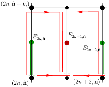
We define the transverse electric fields emanating from the new sites as the average of the parallel transports of the electric fields $\pm 1$ units of $\eta$ away, as shown in Figure 3. We parallel transport the indices of $E^{i}U^{i}$ in the same way as we did with the link matrix $U^{i}$, leading to

Together with our choice of $\widetilde{E}^{\eta}$ fields, this ensures that Gauss’ law is satisfied also at the new (odd-$\hat{\eta}_{\rm new}$) lattice sites — up to corrections which arise due to the failure of $E$ to commute with the magnetic field, which first arise at order $a_{\perp}^{2}a_{\eta}^{2}EB^{2}$. Therefore in the nonabelian context Gauss’ law will not be identically satisfied at the new interpolated lattice sites, though the failure is small and suppressed by $a_{\perp}^{2}a_{\eta}^{2}$. A final step is needed, in which one corrects the electric fields such that Gauss’ law becomes exact. The optimal choice is to change the electric fields by an amount which is strictly the gradient of a scalar potential, and with this choice the shift in the electric fields, to restore Gauss’ law, is unique. We propose to use the algorithm for finding this shift, described in detail in Ref. [11]. This completes the specification of our algorithm for the nonabelian case.

We have presented a new approach to studying classical field theory in a linearly expanding system on the lattice, with intended applications in the study of early-time dynamics after heavy ion collisions. The algorithm allows the evolution to proceed to late times in boxes of large transverse extent, without encountering the problem that the longitudinal ($\eta$) lattice spacing becomes coarse. We do this by periodically cropping the box in the $\eta$ direction and refining the mesh. We have presented a detailed algorithm both for scalars and for nonabelian gauge fields.

In practical applications it will probably be necessary to start the evolution at very early times, perhaps even $\tau\sim a_{\perp}$ but in any case $\tau\ll L_{\perp}$. We do not think it necessary to begin with a range of $\eta$ larger than a few, since few excitations will ever propagate over a range of $\eta$ larger than 1 or 2. Therefore it might make sense to begin with a lattice which does have a large hierarchy $a_{\eta}\ll a_{\perp}$. In this case our cropping and interpolation would only begin when $a_{\eta}\sim a_{\perp}$, at times $\tau\sim L_{\perp}$.

We emphasize again the importance of establishing that simulations, particularly of nonabelian gauge fields, are really in the large $L_{\perp}$ limit. This limit is challenging, because as we emphasized in the introduction, the screening length scale grows as $\tau^{1/2}$. Therefore we expect that our approach will actually be necessary to study sufficiently wide boxes, particularly if the study is to proceed to late times.

We thank Jürgen Berges and Sören Schlichting for useful discussions and giving us an advanced copy of Ref. [8], which inspired this work. This work was supported in part by the Institute for Particle Physics (Canada) and the National Science and Engineering Research Council (NSERC) of Canada.

References

- [1] For reviews see for instance, E. Iancu, R. Venugopalan, In *Hwa, R.C. (ed.) et al.: Quark gluon plasma* 249-363. [hep-ph/0303204]; F. Gelis, E. Iancu, J. Jalilian-Marian and R. Venugopalan, Ann. Rev. Nucl. Part. Sci. 60, 463 (2010) [arXiv:1002.0333 [hep-ph]].
- [2] L. D. McLerran, R. Venugopalan, Phys. Rev. D49, 2233-2241 (1994). [arXiv:hep-ph/9309289 [hep-ph]]; Phys. Rev. D49, 3352-3355 (1994). [hep-ph/9311205]. J. Jalilian-Marian, A. Kovner, L. D. McLerran, H. Weigert, Phys. Rev. D55, 5414-5428 (1997). [hep-ph/9606337].
- [3] A. Kovner, L. D. McLerran, H. Weigert, Phys. Rev. D52, 6231-6237 (1995). [hep-ph/9502289]. A. Krasnitz, R. Venugopalan, Phys. Rev. Lett. 84, 4309-4312 (2000). [hep-ph/9909203]. T. Lappi and L. McLerran, Nucl. Phys. A 772, 200 (2006) [arXiv:hep-ph/0602189].
- [4] A. Krasnitz and R. Venugopalan, Nucl. Phys. B 557, 237 (1999) [hep-ph/9809433].
- [5] A. Krasnitz, Y. Nara and R. Venugopalan, Phys. Rev. Lett. 87, 192302 (2001) [hep-ph/0108092].
- [6] T. Lappi, Phys. Rev. C 67 (2003) 054903 [hep-ph/0303076].
- [7] P. Romatschke and R. Venugopalan, Phys. Rev. Lett. 96, 062302 (2006) [hep-ph/0510121].
- [8] J. Berges and S. Schlichting, arXiv:1209.0817 [hep-ph].
- [9] A. Kurkela and G. D. Moore, arXiv:1207.1663 [hep-ph].
- [10] Y. Liang, K. -F. Liu, B. -A. Li, S. J. Dong and K. Ishikawa, Phys. Lett. B 307, 375 (1993) [hep-lat/9304011].
- [11] G. D. Moore, Nucl. Phys. B 480, 657 (1996) [hep-ph/9603384].