跳到论文正文
W Papers独立论文阅读器 arXiv:1209.4011 论文正文 计算阅读时间 · 0%
引用这篇论文根据当前论文元数据生成,正式投稿前建议核对。


License: arXiv.org perpetual non-exclusive license
arXiv:1209.4011v3 [hep-ph] 05 Aug 2013

into light hadrons with both QCD and relativistic corrections at order O⁡(αs​v2)O(\alpha_{s}v^{2}) in nonrelativistic QCD. With appropriate estimates for the long-distance matrix elements by using the potential model and operator evolution method, we find that our predictions of these decay widths are consistent with recent experimental measurements. We also find that the O⁡(αs​v2)O(\alpha_{s}v^{2}) corrections are small for b​b¯b\overline{b} states but substantial for c​c¯c\overline{c} states. In particular, the negative contribution of O⁡(αs​v2)O(\alpha_{s}v^{2}) correction to the hch_{c} decay can lower the decay width, as compared with previous predictions without the O⁡(αs​v2)O(\alpha_{s}v^{2}) correction, and thus result in a good agreement with the recent BESIII measurement.

QCD and relativistic O⁡(αs​v2)O(\alpha_{s}v^{2}) corrections to hadronic decays of spin-singlet heavy quarkonia hc,hbh_{c},h_{b} and ηb\eta_{b}

Jin-Zhao Li Email: lijinzhao86@gmail.com Affiliation: Department of Physics and State Key Laboratory of Nuclear Physics and Technology,
Peking University, Beijing 100871, China
   Yan-Qing Ma Email: yqma@bnl.gov Affiliation: Physics Department, Brookhaven National Laboratory, Upton, New York 11973, USA    Kuang-Ta Chao Email: ktchao@pku.edu.cn Affiliation: Department of Physics and State Key Laboratory of Nuclear Physics and Technology, and Center for High Energy Physics,
Peking University, Beijing 100871, China
Abstract

We calculate the annihilation decay widths of spin-singlet heavy quarkonia hc,hbh_{c},h_{b} and ηb\eta_{b}

pacs
12.38.Bx, 13.25.Gv, 14.40.Pq

I INTRODUCTION

The inclusive annihilation decay of heavy quarkonium is one of the important issues in heavy quarkonium physics. It is widely accepted that the heavy quarkonium inclusive annihilation decay can be described by nonrelativistic QCD (NRQCD) factorization [1]. In this framework, the long-distance effects that cannot be calculated perturbatively are described by the long-distance matrix elements (LDMEs), which are classified in the order of vv, the relative velocity of heavy quarks in quarkonium. As vv is small in heavy quarkonium system, we need to keep only a few number of LDMEs in the calculation. Recently, more precise measurements for heavy quarkonium decay widths and branching ratios are available  [2, 3, 4, 5, 6, 8, 7, 9, 10, 11, 12]. Thus, it is necessary to provide more precise theoretical predictions to compare with the data.

For charmonium, the c​c¯c\overline{c} system, the inclusive annihilation hadronic decay (into gluons and light quark pairs) widths for SS-, PP-, and DD-wave states are all calculated up to O⁡(αs)O(\alpha_{s}) in NRQCD [13, 14, 15, 16, 17, 19, 18]. Particularly, for the SS-wave state ηc\eta_{c}, the O⁡(αs​v2)O(\alpha_{s}v^{2}) corrections have recently been carried out [20], which means the short-distance coefficients of O⁡(v2)O(v^{2}) LDMEs are calculated perturbatively to next-to-leading order (NLO) in αs\alpha_{s}. After taking the O⁡(αs​v2)O(\alpha_{s}v^{2}) corrections into account, the measurements of ηc\eta_{c} decay can be described much better in NRQCD. For the PP-wave state hch_{c}, the earlier theoretical result at O⁡(αs)O(\alpha_{s}) predicts the hadronic decay width of hch_{c} to be about 0.720.72 MeV[17], which is a factor of 2 larger than the latest measurements by BESIII, where the central value of the total width is about 0.730.73 MeV and the hadronic decay branching ratio is about 50%50\%[5]. Thus it is needed to study higher order in vv corrections to examine whether the gap between theoretical predictions and experimental measurements can be explained. It will be an interesting test for the validity of NRQCD factorization for charmonium system.

For bottomonium, the b​b¯b\overline{b} system, the value of v2v^{2} is about 0.10.1, which is much smaller than v2≈0.3v^{2}\approx 0.3 for charmonium. It is then expected that the v2v^{2} expansion should be better for bottomonium, thus the study of bottomonium is more solid to check NRQCD factorization. Recently, the process hb​(1​P)→ηb​(1​S)​γh_{b}(1P)\rightarrow\eta_{b}(1S)\gamma was measured by the Belle Collaboration [8]. It was found that the ηb\eta_{b} decay width was about 12.412.4 MeV and the decay branching fraction of ℬ[hb(1P)→ηb(1S)γ]=49.2±5.7−3.3+5.6%\mathcal{B}[h_{b}(1P)\rightarrow\eta_{b}(1S)\gamma]=49.2\pm 5.7^{+5.6}_{-3.3}\%. It is tempting to try to explain these data in NRQCD.

In this paper, we will perform the O⁡(αs​v2)O(\alpha_{s}v^{2}) calculations for the spin-singlet PP-wave charmonium hch_{c} and bottomonium hbh_{b}, and also for the spin-singlet SS-wave bottomonium ηb\eta_{b}. We find these corrections are important to understand the measured data. The rest of this paper is organized as follows. In Sec. II we briefly introduce the NRQCD factorization formulism in heavy quarkonium annihilation decays. Then we describe some technical method in calculating O⁡(αs​v2)O(\alpha_{s}v^{2}) short-distance coefficients in Sec.III. The results for SS-wave and PP-wave states including real and virtual contributions are presented in Sec. IV. With these results and appropriate estimates of the LDMEs, we discuss the related phenomenology in Sec. V. In the Appendix A, we calculate the evolution of LDMEs at O⁡(αs​v2)O(\alpha_{s}v^{2}). In the Appnedix B, we describe our factorization scheme choice and show how to eliminate higher twist operators. Finally, we give a brief summary in Sec. VI.

II NRQCD FACTORIZATION FOR QUARKONIUM DECAY

In this section, we introduce the NRQCD factorization formula for the rates of spin-singlet heavy quarkonium (ηc,b\eta_{c,b} and hc,bh_{c,b}) decays to light hadrons. The inclusive annihilation decay width of heavy quarkonium can be factorized by the following formula [1]

Γ⁡(H)=∑n2​ Im​fn​(μΛ)mQdn−4​⟨H|​𝒪n​(μΛ)​|H⟩,\displaystyle\Gamma(H)=\sum_{n}\frac{2\textrm{ Im}f_{n}(\mu_{\Lambda})}{m_{Q}^{d_{n}-4}}\langle H|\mathcal{O}_{n}(\mu_{\Lambda})|H\rangle, (1)

where Im​fn​(μΛ)\textrm{Im}f_{n}(\mu_{\Lambda}) is the short-distance (SD) coefficient that can be perturbatively calculated using full QCD Lagrangian. The LDMEs ⟨H|𝒪n​(μΛ)|H⟩\langle H|\mathcal{O}_{n}(\mu_{\Lambda})|H\rangle involve non-perturbative effects and are classified by the relative velocity vv between QQ and Q¯\overline{Q}, according to power counting in Refs. [1, 21, 23, 22, 24].

The NRQCD Lagrangian can be derived by integrating out the degrees of freedom of order mQm_{Q}, the mass of the heavy quark, from the QCD Lagrangian, which gives

ℒNRQCD=ℒlight+ℒheavy+δ​ℒ.\displaystyle\mathcal{L}_{\textrm{NRQCD}}=\mathcal{L}_{\textrm{light}}+\mathcal{L}_{\textrm{heavy}}+\delta\mathcal{L}. (2)

The heavy part of the Lagrangian describes the motions of (anti-)heavy quark in spacetime and is given by

ℒheavy=ψ†​(i​Dt+𝐃22​mQ)​ψ+χ†​(i​Dt−𝐃22​mQ)​χ\displaystyle\mathcal{L}_{\textrm{heavy}}=\psi^{\dagger}(iD_{t}+\frac{\mathbf{D}^{2}}{2m_{Q}})\psi+\chi^{\dagger}(iD_{t}-\frac{\mathbf{D}^{2}}{2m_{Q}})\chi (3)

where ψ\psi(χ\chi) denotes the Pauli spinor field that annihilates (creates) a heavy (anti-)quark, and DtD_{t}(𝐃\mathbf{D}) is the time(space) component of the gauge-covariant derivative DμD^{\mu}. The light piece of the Lagrangian reads

ℒlight=−12​Tr ​Gμ​ν​Gμ​ν+∑nfq¯​i​D̸​q\displaystyle\mathcal{L}_{\textrm{light}}=-\frac{1}{2}\textrm{Tr }G^{\mu\nu}G_{\mu\nu}+\sum_{n_{f}}\overline{q}i\not{D}q (4)

where Gμ​νG^{\mu\nu} is the gluon field strength tensor, qq is the Dirac spinor field of light quarks and nfn_{f} is the number of light flavors. The bilinear Lagrangian term which contains the order v2v^{2} correction is

δ​𝐋bilinear\displaystyle\delta\mathbf{L}_{\textrm{bilinear}} =\displaystyle= c18​mQ3​ψ†​(𝐃2)2​ψ+c28​mQ2​ψ†​(𝐃⋅g​𝐄−g​𝐄⋅𝐃)​ψ\displaystyle\frac{c_{1}}{8m_{Q}^{3}}\psi^{\dagger}(\mathbf{D}^{2})^{2}\psi+\frac{c_{2}}{8m_{Q}^{2}}\psi^{\dagger}(\mathbf{D}\cdot g\mathbf{E}-g\mathbf{E}\!\cdot\!\mathbf{D})\psi (5)
+\displaystyle+ c38​mQ2​ψ†​(i​𝐃×g​𝐄−g​𝐄×i​𝐃)⋅σ​ψ+c42​mQ​ψ†​(g​𝐁⋅σ)​ψ\displaystyle\frac{c_{3}}{8m_{Q}^{2}}\psi^{\dagger}(i\mathbf{D}\!\times\!g\mathbf{E}-g\mathbf{E}\!\times\!i\mathbf{D})\!\cdot\!\mathbf{\sigma}\psi+\frac{c_{4}}{2m_{Q}}\psi^{\dagger}(g\mathbf{B}\!\cdot\!\mathbf{\sigma})\psi
+\displaystyle+ charge conjugate terms,\displaystyle\textrm{charge conjugate terms},

where Ei=G0​iE^{i}=G^{0i} and Bi=12​ϵi​j​k​Gj​kB^{i}=\frac{1}{2}\epsilon^{ijk}G^{jk} are the electric and magnetic components of the gluon field strength tensor Gμ​νG^{\mu\nu}, and ci=1+O(αs),i=1,2,3,4c_{i}=1+O(\alpha_{s}),i=1,2,3,4 are the dimensionless coefficients corresponding to each operator.

In order to describe the annihilation decay of quarkonium, a set of local four-fermion operators 𝒪i\mathcal{O}_{i} which appear in Eq. (1) are needed. For example, the operator ψ†​χ​χ†​ψ\psi^{\dagger}\chi\chi^{\dagger}\psi can annihilate a Q​Q¯Q\overline{Q} pair in the S[1]01{}^{1}\!S_{0}^{[1]} configuration. In our case, for the O⁡(αs​v2)O(\alpha_{s}v^{2}) calculation of spin-singlet quarkonium decay, the power counting rules [1] give the following seven operators and LDMEs in Eq. (1): for SS-wave quarkonium,

𝒪(1S0[1])\displaystyle\mathcal{O}(^{1}S_{0}^{[1]}) =\displaystyle= ψ†​χ​χ†​ψ,\displaystyle\psi^{\dagger}\chi\chi^{\dagger}\psi, (6a)
𝒫(1S0[1])\displaystyle\mathcal{P}(^{1}S_{0}^{[1]}) =\displaystyle= 12​ψ†​χ​χ†​(−i​𝐃⃡2)2​ψ+h.c.,\displaystyle\frac{1}{2}\psi^{\dagger}\chi\chi^{\dagger}(-\frac{i\tensor{\mathbf{D}}}{2})^{2}\psi+\textrm{h.c.}, (6b)

for PP wave quarkonium,

𝒪(1S0[8])\displaystyle\mathcal{O}(^{1}S_{0}^{[8]}) =\displaystyle= ψ†​Ta​χ​χ†​Ta​ψ,\displaystyle\psi^{\dagger}T^{a}\chi\chi^{\dagger}T^{a}\psi, (7a)
𝒫(1S0[8])\displaystyle\mathcal{P}(^{1}S_{0}^{[8]}) =\displaystyle= 12​ψ†​Ta​χ​χ†​Ta​(−i​𝐃⃡2)2​ψ+h.c.,\displaystyle\frac{1}{2}\psi^{\dagger}T^{a}\chi\chi^{\dagger}T^{a}(-\frac{i\tensor{\mathbf{D}}}{2})^{2}\psi+\textrm{h.c.}, (7b)
𝒪(1P1[1])\displaystyle\mathcal{O}(^{1}P_{1}^{[1]}) =\displaystyle= ψ†​(−i​𝐃⃡2)​χ⋅χ†​(−i​𝐃⃡2)​ψ,\displaystyle\psi^{\dagger}(-\frac{i\tensor{\mathbf{D}}}{2})\chi\!\cdot\!\chi^{\dagger}(-\frac{i\tensor{\mathbf{D}}}{2})\psi, (7c)
𝒫(1P1[1])\displaystyle\mathcal{P}(^{1}P_{1}^{[1]}) =\displaystyle= 12​ψ†​(−i​𝐃⃡2)​χ⋅χ†​(−i​𝐃⃡2)3​ψ+h.c.,\displaystyle\frac{1}{2}\psi^{\dagger}(-\frac{i\tensor{\mathbf{D}}}{2})\chi\!\cdot\!\chi^{\dagger}(-\frac{i\tensor{\mathbf{D}}}{2})^{3}\psi+\textrm{h.c.}, (7d)
𝒯1−8(1S0,1P1)\displaystyle\mathcal{T}_{1-8}(^{1}\!S_{0},^{1}\!P_{1}) =\displaystyle= 12​ψ†​g​𝐄​χ⋅χ†​𝐃⃡​ψ+h.c.,\displaystyle\frac{1}{2}\psi^{\dagger}g\mathbf{E}\chi\cdot\chi^{\dagger}\tensor{\mathbf{D}}\psi+\textrm{h.c.}, (7e)

and

⟨𝒪(2​S+1LJ[1,8])⟩H\displaystyle\langle\mathcal{O}(^{2S+1}\!L_{J}^{[1,8]})\rangle_{H} ≡\displaystyle\equiv ⟨H|𝒪(2​S+1LJ[1,8])|H⟩,\displaystyle\langle H|\mathcal{O}(^{2S+1}\!L_{J}^{[1,8]})|H\rangle, (8a)
⟨𝒫(2​S+1LJ[1,8])⟩H\displaystyle\langle\mathcal{P}(^{2S+1}\!L_{J}^{[1,8]})\rangle_{H} ≡\displaystyle\equiv ⟨H|𝒫(2​S+1LJ[1,8])|H⟩.\displaystyle\langle H|\mathcal{P}(^{2S+1}\!L_{J}^{[1,8]})|H\rangle. (8b)

Note that, choosing different power counting rules, one may get a different set of operators. For example, in the power counting rule of Ref. [24], mQm_{Q} and vv are homogeneous, which gives that the chromomagnetic field g​𝐁g\mathbf{B} scales as (mQ​v)2(m_{Q}v)^{2}. While that field scales as mQ2​v4m_{Q}^{2}v^{4} in Ref. [1], which is further suppressed by v2v^{2}. As a result, many operators considered in Ref. [24] disappear in our calculation, leaving the above seven. These seven matrix elements are all independent with each other, i.e. they cannot be eliminated by field redefinition or Poincare invariance [24].

Using the seven operators, we give the explicit form of Eq. (1) for S01{}^{1}\!S_{0} and P11{}^{1}\!P_{1} states,

Γ(H(1S0)→LH)=F(1S0[1])mQ2⟨𝒪(1S0[1])⟩S01+G(1S0[1])mQ4⟨𝒫(1S0[1])⟩S01,\displaystyle\Gamma(H(^{1}\!S_{0})\rightarrow\textrm{LH})=\frac{F(^{1}\!S_{0}^{[1]})}{m_{Q}^{2}}\langle\mathcal{O}(^{1}\!S_{0}^{[1]})\rangle_{{}^{1}\!S_{0}}+\frac{G(^{1}\!S_{0}^{[1]})}{m_{Q}^{4}}\langle\mathcal{P}(^{1}\!S_{0}^{[1]})\rangle_{{}^{1}\!S_{0}}, (9a)
Γ(H(1P1)→LH)\displaystyle\Gamma(H(^{1}\!P_{1})\rightarrow\textrm{LH}) =\displaystyle= F(1S0[8])mQ2⟨𝒪(1S0[8])⟩P11+G(1S0[8])mQ4⟨𝒫(1S0[8])⟩P11\displaystyle\frac{F(^{1}\!S_{0}^{[8]})}{m_{Q}^{2}}\langle\mathcal{O}(^{1}\!S_{0}^{[8]})\rangle_{{}^{1}\!P_{1}}+\frac{G(^{1}\!S_{0}^{[8]})}{m_{Q}^{4}}\langle\mathcal{P}(^{1}\!S_{0}^{[8]})\rangle_{{}^{1}\!P_{1}} (9b)
+\displaystyle+ F(1P1[1])mQ4⟨𝒪(1P1[1])⟩P11+G(1P1[1])mQ6⟨𝒫(1P1[1])⟩P11.\displaystyle\frac{F(^{1}\!P_{1}^{[1]})}{m_{Q}^{4}}\langle\mathcal{O}(^{1}\!P_{1}^{[1]})\rangle_{{}^{1}\!P_{1}}+\frac{G(^{1}\!P_{1}^{[1]})}{m_{Q}^{6}}\langle\mathcal{P}(^{1}\!P_{1}^{[1]})\rangle_{{}^{1}\!P_{1}}.

Note that, we omit a term of T(1S0,1P1)mQ5⟨𝒯1−8(1S0,1P1)⟩P11\frac{T(^{1}\!S_{0},^{1}\!P_{1})}{m_{Q}^{5}}\langle\mathcal{T}_{1-8}(^{1}\!S_{0},^{1}\!P_{1})\rangle_{{}^{1}\!P_{1}} in Eq. (9b) to simplify our theoretical framework, although the LDME ⟨𝒯1−8(1S0,1P1)⟩P11\langle\mathcal{T}_{1-8}(^{1}\!S_{0},^{1}\!P_{1})\rangle_{{}^{1}\!P_{1}} is of the same order in vv as ⟨𝒫(1P1[1])⟩P11\langle\mathcal{P}(^{1}\!P_{1}^{[1]})\rangle_{{}^{1}\!P_{1}}. There are two reasons that lead us to do this simplification. Numerically, this contribution is small, which is because T(1S0,1P1)T(^{1}\!S_{0},^{1}\!P_{1}) vanishes at leading order (LO) in αs\alpha_{s} due to the charge parity conservation. Theoretically, and more importantly, this contribution is finite, that is, no infrared (IR) poles are needed to cancel between this channel and other four channels in Eq. (9b). It is then impossible to distinguish this finite contribution from the renormalization scheme or factorization scheme choice of other operators, such as ⟨𝒪(1P1[1])⟩P11\langle\mathcal{O}(^{1}\!P_{1}^{[1]})\rangle_{{}^{1}\!P_{1}} or ⟨𝒪(1S0[8])⟩P11\langle\mathcal{O}(^{1}\!S_{0}^{[8]})\rangle_{{}^{1}\!P_{1}}. Therefore, by ignoring this operator in the hadronic decay width, it is equivalent that we choose a specific renormalization scheme or factorization scheme for other operators. In Appendix B, we will give an explicit definition of our factorization scheme to absorb the term T(1S0,1P1)mQ5⟨𝒯1−8(1S0,1P1)⟩P11\frac{T(^{1}\!S_{0},^{1}\!P_{1})}{m_{Q}^{5}}\langle\mathcal{T}_{1-8}(^{1}\!S_{0},^{1}\!P_{1})\rangle_{{}^{1}\!P_{1}}. Although our scheme is in principle distinguished from MS¯{\overline{\text{MS}}} scheme, as we will discussed in Appendix B, there is no difference between these two schemes for our purpose in this work. As a result, we will pretend to use MS¯{\overline{\text{MS}}} scheme in the following.

Through the above factorization formula, one can match full QCD with NRQCD to get the short-distance (SD) coefficients FF and GG perturbatively. The skeleton of the matching procedure is given by

Imℳ(QQ¯→QQ¯)|pert QCD=∑n2 Imfn(μΛ)mQdn−4⟨QQ¯|𝒪n(μΛ)|QQ¯⟩|NRQCD,\displaystyle\textrm{Im}\mathcal{M}(Q\overline{Q}\rightarrow Q\overline{Q})\Big|_{\textrm{pert QCD}}=\sum_{n}\frac{2\textrm{ Im}f_{n}(\mu_{\Lambda})}{m_{Q}^{d_{n}-4}}\langle Q\overline{Q}|\mathcal{O}_{n}(\mu_{\Lambda})|Q\overline{Q}\rangle\Big|_{\textrm{NRQCD}}, (10)

The determination of SD coefficients will be discussed in detail in the next section.

III DETAILS IN FULL QCD CALCULATION

III.1 Kinematics

We work in the rest frame of the heavy quarkonium. It is customary to decompose the momenta of QQ and Q¯\overline{Q} as

pQ\displaystyle p_{Q} =\displaystyle= 12​P+q,\displaystyle\frac{1}{2}P+q, (11a)
pQ¯\displaystyle p_{\overline{Q}} =\displaystyle= 12​P−q,\displaystyle\frac{1}{2}P-q, (11b)

where PP is the total momentum and qq is half of the relative momentum, which satisfies the relation P⋅q=0P\!\cdot\!q=0. The explicit four-vector form of PP and qq in the rest frame are

P\displaystyle P =\displaystyle= (2​E𝐪,𝟎),\displaystyle(2E_{\mathbf{q}},\mathbf{0}), (12a)
q\displaystyle q =\displaystyle= (0,𝐪),\displaystyle(0,\mathbf{q}), (12b)

with E𝐪=mQ2+𝐪2E_{\mathbf{q}}=\sqrt{m_{Q}^{2}+\mathbf{q}^{2}}.

The treatment of final state phase space integration at O⁡(αs​v2)O(\alpha_{s}v^{2}) level is slightly different from ordinary calculations (i.e. leading order of vv calculation). To make it simpler, we use the following rescaling transformation for all external momenta [25, 20],

P\displaystyle P →\displaystyle\rightarrow P′​E𝐪mQ,\displaystyle P^{\prime}\frac{E_{\mathbf{q}}}{m_{Q}}, (13a)
kf\displaystyle k_{f} →\displaystyle\rightarrow kf′​E𝐪mQ,\displaystyle k_{f}^{\prime}\frac{E_{\mathbf{q}}}{m_{Q}}, (13b)

but keep the relative momentum qq and loop integral momentum ll unchanged. Once we take such trick, the 𝐪2\mathbf{q}^{2} dependence in both phase space and current factor [i.e. 1/(2​M)1/(2M) where MM is the quarkonium mass] can be absorbed into the amplitude, then we can safely take 𝐪→0\mathbf{q}\rightarrow 0 in these terms and only expand 𝐪,𝐪′\mathbf{q},\mathbf{q}^{\prime} at the amplitude level, where 𝐪′\mathbf{q}^{\prime} is half of the relative momentum between Q​Q¯Q\overline{Q} pair on the complex conjugate side. (Note that |𝐪|=|𝐪′||\mathbf{q}|=|\mathbf{q}^{\prime}| but their direction does not need to be the same, so in general 𝐪≠𝐪′\mathbf{q}\neq\mathbf{q}^{\prime}). It should be kept in mind that this trick can only work in the case where all final state partons are massless (i.e. gluons and light quarks), because, in the case of massive partons, the on-shell relation does not hold under rescaling, which will break the QCD gauge invariance.

III.2 Covariant Projection Method in D-Dimension

Instead of using matching method directly, we use an equivalent but more efficient method, i.e., the covariant projection method, to calculate the imaginary part of the SD coefficients in Eqs. (9a) and (9b). In order to get spin-singlet Q​Q¯Q\overline{Q} decay amplitudes, we take the following spin and color projectors onto Q​Q¯Q\overline{Q} quark lines [26]:

Π0=12​2​(E𝐪+mQ)​(P̸2+q̸+mQ)​(P̸+2​E𝐪)​γ5​(−P̸+2​E𝐪)8​E𝐪2​(P̸2−q̸−mQ),\displaystyle\Pi_{0}=\frac{1}{2\sqrt{2}(E_{\mathbf{q}}+m_{Q})}(\frac{\not{P}}{2}+\not{q}+m_{Q})\frac{(\not{P}+2E_{\mathbf{q}})\gamma_{5}(-\not{P}+2E_{\mathbf{q}})}{8E_{\mathbf{q}}^{2}}(\frac{\not{P}}{2}-\not{q}-m_{Q}), (14)

and

𝒞1\displaystyle\mathcal{C}_{1} =\displaystyle= 𝟏Nc,\displaystyle\frac{\mathbf{1}}{\sqrt{N_{c}}}, (15a)
𝒞8\displaystyle\mathcal{C}_{8} =\displaystyle= 2​𝐓a.\displaystyle\sqrt{2}\mathbf{T}^{a}. (15b)

We do Taylor expansion of the projected amplitudes in powers of qq to the required order,

ℳ⁡(q)\displaystyle\mathcal{M}(q) =\displaystyle= ℳ⁡(0)+∂ℳ⁡(q)∂qα|q=0​qα+12!​∂2ℳ⁡(q)∂qα​∂qβ|q=0​qα​qβ\displaystyle\mathcal{M}(0)+\frac{\partial\mathcal{M}(q)}{\partial q^{\alpha}}\Big|_{q=0}q^{\alpha}+\frac{1}{2!}\frac{\partial^{2}\mathcal{M}(q)}{\partial q^{\alpha}\partial q^{\beta}}\Big|_{q=0}q^{\alpha}q^{\beta} (16)
+\displaystyle+ 13!​∂3ℳ⁡(q)∂qα​∂qβ​∂qγ|q=0​qα​qβ​qγ+⋯,\displaystyle\frac{1}{3!}\frac{\partial^{3}\mathcal{M}(q)}{\partial q^{\alpha}\partial q^{\beta}\partial q^{\gamma}}\Big|_{q=0}q^{\alpha}q^{\beta}q^{\gamma}+\cdots,

and then make the replacement:

qα​qβ\displaystyle q_{\alpha}q_{\beta} →\displaystyle\rightarrow 𝐪2D−1​Πα​β,\displaystyle\frac{\mathbf{q}^{2}}{D-1}\Pi_{\alpha\beta}, (17a)
qα​qβ′\displaystyle q_{\alpha}q_{\beta}^{\prime} →\displaystyle\rightarrow 𝐪⋅𝐪′D−1​Πα​β,\displaystyle\frac{\mathbf{q}\!\cdot\!\mathbf{q}^{\prime}}{D-1}\Pi_{\alpha\beta}, (17b)
qα​qβ​qγ​qλ′\displaystyle q_{\alpha}q_{\beta}q_{\gamma}q_{\lambda}^{\prime} →\displaystyle\rightarrow 𝐪2​𝐪⋅𝐪′D+1​(Πα​β​Πγ​λ+Πα​γ​Πβ​λ+Πα​λ​Πγ​β),\displaystyle\frac{\mathbf{q}^{2}\mathbf{q}\!\cdot\!\mathbf{q}^{\prime}}{D+1}(\Pi_{\alpha\beta}\Pi_{\gamma\lambda}+\Pi_{\alpha\gamma}\Pi_{\beta\lambda}+\Pi_{\alpha\lambda}\Pi_{\gamma\beta}), (17c)

to project them to definite states, where

Πα​β=−gα​β+Pα′​Pβ′4​mQ2,\Pi_{\alpha\beta}=-g_{\alpha\beta}+\frac{P_{\alpha}^{\prime}P_{\beta}^{\prime}}{4m_{Q}^{2}}, (18)

with P′P^{\prime} the rescaled heavy quarkonium momentum. For example, the third derivative term of ℳ\mathcal{M} convolutes with the first derivative term of ℳ†\mathcal{M}^{\dagger} giving the squared amplitudes term,

13!​∂3ℳ⁡(q)∂qα​∂qβ​∂qγ|q=0​∂ℳ†​(q′)∂q′λ|q′=0​qα​qβ​qγ​q′λ\displaystyle\frac{1}{3!}\frac{\partial^{3}\mathcal{M}(q)}{\partial q^{\alpha}\partial q^{\beta}\partial q^{\gamma}}\Big|_{q=0}\frac{\partial\mathcal{M}^{\dagger}(q^{\prime})}{\partial q^{\prime\lambda}}\Big|_{q^{\prime}=0}q^{\alpha}q^{\beta}q^{\gamma}q^{\prime\lambda} (19)
→\displaystyle\rightarrow 13!​𝐪2​𝐪⋅𝐪′D+1​(Πα​β​Πγ​λ+Πα​γ​Πβ​λ+Πα​λ​Πγ​β)​∂3ℳ⁡(q)∂qα​∂qβ​∂qγ|q=0​∂ℳ†​(q′)∂q′λ|q′=0\displaystyle\frac{1}{3!}\frac{\mathbf{q}^{2}\mathbf{q}\!\cdot\!\mathbf{q}^{\prime}}{D+1}(\Pi_{\alpha\beta}\Pi_{\gamma\lambda}+\Pi_{\alpha\gamma}\Pi_{\beta\lambda}+\Pi_{\alpha\lambda}\Pi_{\gamma\beta})\frac{\partial^{3}\mathcal{M}(q)}{\partial q^{\alpha}\partial q^{\beta}\partial q^{\gamma}}\Big|_{q=0}\frac{\partial\mathcal{M}^{\dagger}(q^{\prime})}{\partial q^{\prime\lambda}}\Big|_{q^{\prime}=0}

which contributes to the SD coefficient of G(1P1[1])G(^{1}P_{1}^{[1]}) in Eq. (9b).

IV PERTURBATIVE QCD RESULTS OF SHORT-DISTANCE COEFFICIENTS

We generate Feynman diagrams and amplitudes by FeynArts [27, 28], and then calculate the squared amplitudes by self-written Mathematica codes. The phase space integrals are done analytically using the method presented in Ref. [16]. Ultra-violet(UV) and IR divergences are both regularized by dimensional regularization. The renormalizations for heavy quark mass mQm_{Q}, heavy quark field ψQ\psi_{Q}, light quark field ψq\psi_{q} and gluon field AμA_{\mu} are in the on-mass-shell scheme(OS), and that for the QCD coupling constant gsg_{s} is in the M​S¯\overline{MS} scheme,

δ​ZmQO​S\displaystyle\delta Z_{m_{Q}}^{OS} =\displaystyle= −3​CF​αs4​π​Nϵ​[1ϵU​V+43],\displaystyle-3C_{F}\frac{\alpha_{s}}{4\pi}N_{\epsilon}\left[\frac{1}{\epsilon_{UV}}+\frac{4}{3}\right], (20a)
δ​Z2O​S\displaystyle\delta Z_{2}^{OS} =\displaystyle= −CF​αs4​π​Nϵ​[1ϵU​V+2ϵI​R+4],\displaystyle-C_{F}\frac{\alpha_{s}}{4\pi}N_{\epsilon}\left[\frac{1}{\epsilon_{UV}}+\frac{2}{\epsilon_{IR}}+4\right], (20b)
δ​Z2​lO​S\displaystyle\delta Z_{2l}^{OS} =\displaystyle= −CF​αs4​π​Nϵ​[1ϵU​V−1ϵI​R],\displaystyle-C_{F}\frac{\alpha_{s}}{4\pi}N_{\epsilon}\left[\frac{1}{\epsilon_{UV}}-\frac{1}{\epsilon_{IR}}\right], (20c)
δ​Z3O​S\displaystyle\delta Z_{3}^{OS} =\displaystyle= αs4​π​Nϵ​[(β0−2​CA)​(1ϵU​V−1ϵI​R)],\displaystyle\frac{\alpha_{s}}{4\pi}N_{\epsilon}\left[(\beta_{0}-2C_{A})\left(\frac{1}{\epsilon_{UV}}-\frac{1}{\epsilon_{IR}}\right)\right], (20d)
δ​ZgM​S¯\displaystyle\delta Z_{g}^{\overline{MS}} =\displaystyle= −β02​αs4​π​Nϵ​[1ϵU​V+ln⁡mQ2μr2],\displaystyle-\frac{\beta_{0}}{2}\frac{\alpha_{s}}{4\pi}N_{\epsilon}\left[\frac{1}{\epsilon_{UV}}+\ln\frac{m_{Q}^{2}}{\mu_{r}^{2}}\right], (20e)

where Nϵ​(mQ)=(4​π​μr2mQ2)ϵ​Γ​(1+ϵ)N_{\epsilon}(m_{Q})=(\frac{4\pi\mu_{r}^{2}}{m_{Q}^{2}})^{\epsilon}\Gamma(1+\epsilon) is an overall factor, and μr\mu_{r} is the renormalization scale. β0=113​CA−43​TF​nf\beta_{0}=\frac{11}{3}C_{A}-\frac{4}{3}T_{F}n_{f} is the one-loop coefficient of the β\beta function, nfn_{f} is the active quark flavors, which we set to be 3 for charmonium and 4 for bottomonium.

IV.1 Short-Distance Coefficients of S-Wave Quarkonium Hadronic Decay

Leading order in αs\alpha_{s} calculations give the Born level decay width and its relativistic correction, respectively, as

ΓBorn(1S0[1]→gg)\displaystyle\Gamma_{\mbox{{\footnotesize Born}}}(^{1}\!S_{0}^{[1]}\rightarrow gg) =\displaystyle= 43​(4​π​αs)2​μr4​ϵmQ2​Φ(2)​(1−ϵ)​(1−2​ϵ)​⟨𝒪(1S0[1])⟩S01Born2​Nc,\displaystyle\frac{4}{3}(4\pi\alpha_{s})^{2}\frac{\mu_{r}^{4\epsilon}}{m_{Q}^{2}}\Phi_{(2)}(1-\epsilon)(1-2\epsilon)\frac{\langle\mathcal{O}(^{1}\!S_{0}^{[1]})\rangle_{{}^{1}\!S_{0}}^{\mbox{{\footnotesize Born}}}}{2N_{c}}, (21a)
ΓBorn(v2)(1S0[1]→gg)\displaystyle\Gamma_{\mbox{{\footnotesize Born}}}^{(v^{2})}(^{1}\!S_{0}^{[1]}\rightarrow gg) =\displaystyle= −2​(2−ϵ)3−2​ϵ𝐪2mQ2ΓBorn(1S0[1]→gg),\displaystyle-\frac{2(2-\epsilon)}{3-2\epsilon}\frac{\mathbf{q}^{2}}{m_{Q}^{2}}\Gamma_{\mbox{{\footnotesize Born}}}(^{1}\!S_{0}^{[1]}\rightarrow gg), (21b)

where Φ(2)=18​π​(4​πM2)ϵ​Γ⁡(1−ϵ)Γ⁡(2−2​ϵ)\Phi_{(2)}=\frac{1}{8\pi}(\frac{4\pi}{M^{2}})^{\epsilon}\frac{\Gamma(1-\epsilon)}{\Gamma(2-2\epsilon)} is the total two-body phase space in DD dimension and M=2​mQ​1+𝐪2mQ2M=2m_{Q}\sqrt{1+\frac{\mathbf{q}^{2}}{m_{Q}^{2}}} is the quarkonium mass including the relativistic correction. The two Born diagrams are illustrated in Fig. 1.

Refer to caption
Figure 1: Born level Feynman diagrams for 1S0[1],1S0[8]→gg{}^{1}\!S_{0}^{[1]},^{1}\!S_{0}^{[8]}\rightarrow gg.

The next-to-leading order calculations include real and virtual corrections. For SS-wave Fock states (i.e. S[1]01{}^{1}\!S_{0}^{[1]} and S[8]01{}^{1}\!S_{0}^{[8]}), UV divergences will be canceled by counterterm diagrams, and most IR divergences will be canceled between real and virtual corrections, leaving some residue divergences at O⁡(v2)O(v^{2}). The cancelation of such residue divergences will be presented in the next section by calculating NRQCD LDMEs at one-loop level. The contribution of virtual plus counterterm corrections is

ΓVirtual(1S0[1]→gg)=3​αsπΓBorn(1S0[1]→gg)fϵ(mQ){[−1ϵ2−16β01ϵ+136(−6β0ln(4​mQ2μr2)+19π2−44)]+𝐪2mQ2[431ϵ2−4​nf−97271ϵ−1324(−72β0ln(4​mQ2μr2)+8nf+267π2−280)]},\displaystyle\begin{split}\Gamma_{\mbox{{\footnotesize Virtual}}}(^{1}\!S_{0}^{[1]}\rightarrow gg)=&\frac{3\alpha_{s}}{\pi}\Gamma_{\mbox{{\footnotesize Born}}}(^{1}\!S_{0}^{[1]}\rightarrow gg)f_{\epsilon}(m_{Q})\Big\{[-\frac{1}{\epsilon^{2}}-\frac{1}{6}\beta_{0}\frac{1}{\epsilon}\\ &+\frac{1}{36}(-6\beta_{0}\ln(\frac{4m_{Q}^{2}}{\mu_{r}^{2}})+19\pi^{2}-44)]\\ &+\frac{\mathbf{q}^{2}}{m_{Q}^{2}}[\frac{4}{3}\frac{1}{\epsilon^{2}}-\frac{4n_{f}-97}{27}\frac{1}{\epsilon}\\ &-\frac{1}{324}(-72\beta_{0}\ln(\frac{4m_{Q}^{2}}{\mu_{r}^{2}})+8n_{f}+267\pi^{2}-280)]\Big\},\end{split} (22)

where fϵ​(mQ)=(π​μr2mQ2)ϵ​Γ​(1+ϵ)f_{\epsilon}(m_{Q})=(\frac{\pi\mu_{r}^{2}}{m_{Q}^{2}})^{\epsilon}\Gamma(1+\epsilon). Some selected Feynman diagrams are shown in Fig. 2.
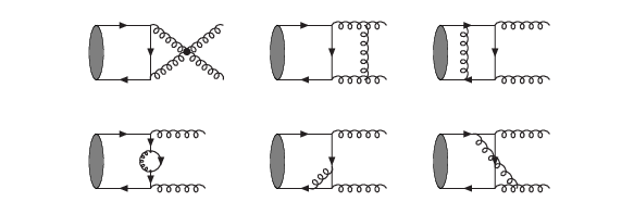
Refer to caption
Figure 2: Virtual correction Feynman diagrams for 1S0[1],1S0[8]→gg{}^{1}\!S_{0}^{[1]},^{1}\!S_{0}^{[8]}\rightarrow gg. The crossed diagrams have been suppressed.

The real correction contains two sets, where one set is the final states with g​g​gggg and the other one with q​q¯​gq\overline{q}g. Some typical Feynman diagrams are shown in Fig. 4 and Fig. 4 and the contributions to decay width are

Refer to caption
Figure 3: Real correction Feynman diagrams for 1S0[1],1S0[8],1P1[1]→ggg{}^{1}\!S_{0}^{[1]},^{1}\!S_{0}^{[8]},^{1}\!P_{1}^{[1]}\rightarrow ggg. The crossed diagrams have been suppressed. The second diagram vanishes in P[1]11{}^{1}\!P_{1}^{[1]}.
Refer to caption
Figure 4: Real correction Feynman diagrams for 1S0[1],1S0[8]→qq¯g{}^{1}\!S_{0}^{[1]},^{1}\!S_{0}^{[8]}\rightarrow q\overline{q}g. The crossed diagrams have been suppressed.
Γ(1S0[1]→ggg)=3​αsπΓBorn(1S0[1]→gg)fϵ(mQ){[1ϵ2+1161ϵ+172(724−69π2)]+𝐪2mQ2[−431ϵ2−3ϵ−437−42​π227]},\displaystyle\begin{split}\Gamma(^{1}\!S_{0}^{[1]}\rightarrow ggg)=&\frac{3\alpha_{s}}{\pi}\Gamma_{\mbox{{\footnotesize Born}}}(^{1}\!S_{0}^{[1]}\rightarrow gg)f_{\epsilon}(m_{Q})\Big\{[\frac{1}{\epsilon^{2}}+\frac{11}{6}\frac{1}{\epsilon}+\frac{1}{72}(724-69\pi^{2})]\\ &+\frac{\mathbf{q}^{2}}{m_{Q}^{2}}[-\frac{4}{3}\frac{1}{\epsilon^{2}}-\frac{3}{\epsilon}-\frac{437-42\pi^{2}}{27}]\Big\},\end{split} (23a)
Γ(1S0[1]→qq¯g)=\displaystyle\Gamma(^{1}\!S_{0}^{[1]}\rightarrow q\overline{q}g)= nf2αsπΓBorn(1S0[1]→gg)fϵ​(mQ)Γ⁡(1+ϵ)​Γ​(1−ϵ)[−231ϵ−169+𝐪2mQ2(891ϵ+8627)].\displaystyle\frac{n_{f}}{2}\frac{\alpha_{s}}{\pi}\Gamma_{\mbox{{\footnotesize Born}}}(^{1}\!S_{0}^{[1]}\rightarrow gg)\frac{f_{\epsilon}(m_{Q})}{\Gamma(1+\epsilon)\Gamma(1-\epsilon)}[-\frac{2}{3}\frac{1}{\epsilon}-\frac{16}{9}+\frac{\mathbf{q}^{2}}{m_{Q}^{2}}(\frac{8}{9}\frac{1}{\epsilon}+\frac{86}{27})]. (23b)

Combining Eqs. (21), (22) and (23), we obtain the hadronic decay width with both QCD radiative and relativistic corrections at NLO of S01{}^{1}\!S_{0} heavy quarkonium,

ΓQCD(1S0→LH)=ΓBorn(1S0[1]→gg){[1+αsπfϵ(mQ)172(−36β0ln(4​mQ2μr2)−64nf−93π2+1908)]−43𝐪2mQ2[1+αsπfϵ(mQ)(−431ϵ+1144(−72β0ln(4​mQ2μr2)−164nf−237π2+4964))]}.\displaystyle\begin{split}\Gamma_{\mbox{\footnotesize QCD}}(^{1}\!S_{0}\rightarrow\mbox{LH})=&\Gamma_{\mbox{{\footnotesize Born}}}(^{1}\!S_{0}^{[1]}\rightarrow gg)\Big\{\big[1+\frac{\alpha_{s}}{\pi}f_{\epsilon}(m_{Q})\frac{1}{72}(-36\beta_{0}\ln(\frac{4m_{Q}^{2}}{\mu_{r}^{2}})\\ &-64n_{f}-93\pi^{2}+1908)\big]-\frac{4}{3}\frac{\mathbf{q}^{2}}{m_{Q}^{2}}\big[1+\frac{\alpha_{s}}{\pi}f_{\epsilon}(m_{Q})(-\frac{4}{3}\frac{1}{\epsilon}\\ &+\frac{1}{144}(-72\beta_{0}\ln(\frac{4m_{Q}^{2}}{\mu_{r}^{2}})-164n_{f}-237\pi^{2}+4964))\big]\Big\}.\end{split} (24)

We note that our results agree with the previous work for O⁡(αs​v2)O(\alpha_{s}v^{2}) correction [20] and O⁡(αs)O(\alpha_{s}) correction [16, 19]. Comparing our results with Ref. [20], a slight difference of two body phase space Φ2\Phi_{2} between them can be found. In Ref. [20] Φ2\Phi_{2} is defined so as to remove the 𝐪2\mathbf{q}^{2} dependence into the coefficients, so our individual virtual and real parts, Eqs. (22) and (23), look different from the results in Ref. [20], but essentially they are equivalent. The total NLO result Eq. (24) is explicitly the same, independent of the definition of Φ2\Phi_{2}. The correct repetition of the hadronic decay SD coefficients of S01{}^{1}\!S_{0} heavy quarkonium enables us to extend discussion from charm quark system to bottom quark system (i.e. ηb\eta_{b}) and also partly checks our codes when dealing with PP-wave heavy quarkonium.

IV.2 Short-Distance Coefficients of P-Wave Quarkonium Hadronic Decay

The procedure in calculating the P11{}^{1}\!P_{1} heavy quarkonium is similar to S01{}^{1}\!S_{0}, although more complicated. Additional simplification can be taken by imposing CC (charge) parity conservation of QCD to constrain Feynman diagrams. A straightforward result is that CC parity conservation prohibits P[1]11{}^{1}\!P_{1}^{[1]} Fock state, which has C=−1C=-1, to decay to two gluons, whose C=+1C=+1, no matter they are real or virtual. By tedious but straightforward calculation, we get the results as follows.

At the Born level,

ΓBorn(1S0[8]→gg)\displaystyle\Gamma_{\mbox{{\footnotesize Born}}}(^{1}\!S_{0}^{[8]}\rightarrow gg) =\displaystyle= 512(4παs)2μr4​ϵmQ2Φ(2)(1−ϵ)(1−2ϵ)⟨𝒪(1S0[8])⟩P11Born,\displaystyle\frac{5}{12}(4\pi\alpha_{s})^{2}\frac{\mu_{r}^{4\epsilon}}{m_{Q}^{2}}\Phi_{(2)}(1-\epsilon)(1-2\epsilon)\langle\mathcal{O}(^{1}\!S_{0}^{[8]})\rangle_{{}^{1}\!P_{1}}^{\mbox{{\footnotesize Born}}}, (25a)
ΓBorn(v2)(1S0[8]→gg)\displaystyle\Gamma_{\mbox{{\footnotesize Born}}}^{(v^{2})}(^{1}\!S_{0}^{[8]}\rightarrow gg) =\displaystyle= −2​(2−ϵ)3−2​ϵ𝐪2mQ2ΓBorn(1S0[8]→gg),\displaystyle-\frac{2(2-\epsilon)}{3-2\epsilon}\frac{\mathbf{q}^{2}}{m_{Q}^{2}}\Gamma_{\mbox{{\footnotesize Born}}}(^{1}\!S_{0}^{[8]}\rightarrow gg), (25b)

For NLO corrections,

ΓVirtual(1S0[8]→gg)=3​αsπΓBorn(1S0[8]→gg)fϵ(mQ){[−1ϵ2+nf−2191ϵ+172(−12β0ln(4​mQ2μr2)+29π2−16)]+𝐪2mQ2[431ϵ2−4​nf−115271ϵ−1628(−144β0ln(4​mQ2μr2)+16nf+345π2−992)]},\displaystyle\begin{split}\Gamma_{\mbox{{\footnotesize Virtual}}}(^{1}\!S_{0}^{[8]}\rightarrow gg)=&\frac{3\alpha_{s}}{\pi}\Gamma_{\mbox{{\footnotesize Born}}}(^{1}\!S_{0}^{[8]}\rightarrow gg)f_{\epsilon}(m_{Q})\Big\{[-\frac{1}{\epsilon^{2}}+\frac{n_{f}-21}{9}\frac{1}{\epsilon}\\ &+\frac{1}{72}(-12\beta_{0}\ln(\frac{4m_{Q}^{2}}{\mu_{r}^{2}})+29\pi^{2}-16)]\\ &+\frac{\mathbf{q}^{2}}{m_{Q}^{2}}[\frac{4}{3}\frac{1}{\epsilon^{2}}-\frac{4n_{f}-115}{27}\frac{1}{\epsilon}\\ &-\frac{1}{628}(-144\beta_{0}\ln(\frac{4m_{Q}^{2}}{\mu_{r}^{2}})+16n_{f}+345\pi^{2}-992)]\Big\},\end{split} (26)
Γ(1S0[8]→ggg)=3​αsπΓBorn(1S0[8]→gg)fϵ(mQ){[1ϵ2+731ϵ−π2+1049]+𝐪2mQ2[−431ϵ2−4ϵ−554−45​π227]},\displaystyle\begin{split}\Gamma(^{1}\!S_{0}^{[8]}\rightarrow ggg)=&\frac{3\alpha_{s}}{\pi}\Gamma_{\mbox{{\footnotesize Born}}}(^{1}\!S_{0}^{[8]}\rightarrow gg)f_{\epsilon}(m_{Q})\Big\{[\frac{1}{\epsilon^{2}}+\frac{7}{3}\frac{1}{\epsilon}-\pi^{2}+\frac{104}{9}]\\ &+\frac{\mathbf{q}^{2}}{m_{Q}^{2}}[-\frac{4}{3}\frac{1}{\epsilon^{2}}-\frac{4}{\epsilon}-\frac{554-45\pi^{2}}{27}]\Big\},\end{split} (27)
Γ(1S0[8]→qq¯g)=\displaystyle\Gamma(^{1}\!S_{0}^{[8]}\rightarrow q\overline{q}g)= nf2αsπΓBorn(1S0[8]→gg)fϵ​(mQ)Γ⁡(1+ϵ)​Γ​(1−ϵ)[−231ϵ−169+𝐪2mQ2(891ϵ+8627)],\displaystyle\frac{n_{f}}{2}\frac{\alpha_{s}}{\pi}\Gamma_{\mbox{{\footnotesize Born}}}(^{1}\!S_{0}^{[8]}\rightarrow gg)\frac{f_{\epsilon}(m_{Q})}{\Gamma(1+\epsilon)\Gamma(1-\epsilon)}[-\frac{2}{3}\frac{1}{\epsilon}-\frac{16}{9}+\frac{\mathbf{q}^{2}}{m_{Q}^{2}}(\frac{8}{9}\frac{1}{\epsilon}+\frac{86}{27})], (28)
Γ(1P1[1]→ggg)=40​αs327fϵ(mQ)(8πΦ2){[−1ϵ+7​π224−53]+𝐪2mQ2[29151ϵ+4216−555​π2900]}⟨𝒪(1P1[1])⟩P11Born2​Nc​mQ4,\displaystyle\begin{split}\Gamma(^{1}\!P_{1}^{[1]}\rightarrow ggg)=&\frac{40\alpha_{s}^{3}}{27}f_{\epsilon}(m_{Q})(8\pi\Phi_{2})\Big\{[-\frac{1}{\epsilon}+\frac{7\pi^{2}}{24}-\frac{5}{3}]\\ &+\frac{\mathbf{q}^{2}}{m_{Q}^{2}}[\frac{29}{15}\frac{1}{\epsilon}+\frac{4216-555\pi^{2}}{900}]\Big\}\frac{\langle\mathcal{O}(^{1}\!P_{1}^{[1]})\rangle_{{}^{1}\!P_{1}}^{\mbox{{\footnotesize Born}}}}{2N_{c}m_{Q}^{4}},\end{split} (29)

Summing over the above results, we get the total hadronic decay width,

ΓQCD(1P1→LH)=ΓBorn(1S0[8]→gg){[1+αsπfϵ(mQ)(−12β0ln(4​mQ2μr2)−89nf−43​π224+34]−43𝐪2mQ2[1+αsπfϵ(mQ)(−7121ϵ+1288(−144β0ln(4​mQ2μr2)−328nf−735π2+12304))]}+40​αs327fϵ(mQ)(8πΦ2){[−1ϵ+7​π224−53]+𝐪2mQ2[29151ϵ+4216−555​π2900]}⟨𝒪(1P1[1])⟩P11Born2​Nc​mQ4.\displaystyle\begin{split}\Gamma_{\mbox{\footnotesize QCD}}(^{1}\!P_{1}\rightarrow\mbox{LH})=&\Gamma_{\mbox{{\footnotesize Born}}}(^{1}\!S_{0}^{[8]}\rightarrow gg)\Big\{\big[1+\frac{\alpha_{s}}{\pi}f_{\epsilon}(m_{Q})(-\frac{1}{2}\beta_{0}\ln(\frac{4m_{Q}^{2}}{\mu_{r}^{2}})\\ &-\frac{8}{9}n_{f}-\frac{43\pi^{2}}{24}+34\big]-\frac{4}{3}\frac{\mathbf{q}^{2}}{m_{Q}^{2}}\big[1+\frac{\alpha_{s}}{\pi}f_{\epsilon}(m_{Q})(-\frac{7}{12}\frac{1}{\epsilon}\\ &+\frac{1}{288}(-144\beta_{0}\ln(\frac{4m_{Q}^{2}}{\mu_{r}^{2}})-328n_{f}-735\pi^{2}+12304))\big]\Big\}\\ &+\frac{40\alpha_{s}^{3}}{27}f_{\epsilon}(m_{Q})(8\pi\Phi_{2})\Big\{[-\frac{1}{\epsilon}+\frac{7\pi^{2}}{24}-\frac{5}{3}]\\ &+\frac{\mathbf{q}^{2}}{m_{Q}^{2}}[\frac{29}{15}\frac{1}{\epsilon}+\frac{4216-555\pi^{2}}{900}]\Big\}\frac{\langle\mathcal{O}(^{1}\!P_{1}^{[1]})\rangle_{{}^{1}\!P_{1}}^{\mbox{{\footnotesize Born}}}}{2N_{c}m_{Q}^{4}}.\end{split} (30)

IV.3 Evaluating NRQCD LDMEs And Matching Full QCD Results

In Eqs. (24) and (30), there exist explicit IR divergences. To cancel these divergence, we need to evaluate LDMEs at the loop level. By replacing all the Born LDMEs appearing in Eqs. (24) and (30) by one-loop LDMEs, all IR divergences should be canceled and the final results will be infra-red safe quantities.

The self-energy contributions that connect Born LDMEs to their corresponding relativistic ones are first calculated in Ref. [1]. The intersecting diagrams that describe the E1 transition between S[8]01{}^{1}\!S_{0}^{[8]} and P[1]11{}^{1}\!P_{1}^{[1]} states at O⁡(αs​v2)O(\alpha_{s}v^{2}) in this work are new. The detailed calculation is presented in Appendix A. Here we give the relevant results in dimensional regularization with M​S¯\overline{MS} renormalization scheme,

⟨𝒪(1S0[1])⟩S01Born→\displaystyle\langle\mathcal{O}(^{1}\!S_{0}^{[1]})\rangle_{{}^{1}\!S_{0}}^{\mbox{{\footnotesize Born}}}\rightarrow ⟨𝒪(1S0[1])⟩S01(μΛ){1−43𝐪2mQ24​αs3​πfϵ(mQ)[1ϵ−ln(μΛ24​mQ2)]},\displaystyle\langle\mathcal{O}(^{1}\!S_{0}^{[1]})\rangle_{{}^{1}\!S_{0}}^{(\mu_{\Lambda})}\Big\{1-\frac{4}{3}\frac{\mathbf{q}^{2}}{m_{Q}^{2}}\frac{4\alpha_{s}}{3\pi}f_{\epsilon}(m_{Q})[\frac{1}{\epsilon}-\ln(\frac{\mu_{\Lambda}^{2}}{4m_{Q}^{2}})]\Big\}, (31a)
⟨𝒪(1S0[8])⟩P11Born→⟨𝒪(1S0[8])⟩P11(μΛ){1−43𝐪2mQ27​αs12​πfϵ(mQ)[1ϵ−ln(μΛ24​mQ2)]}+16​αs9​πfϵ(mQ){[1ϵ−ln(μΛ24​mQ2)]+3​𝐪25​mQ2[−1ϵ+ln(μΛ24​mQ2)]}⟨𝒪(1P1[1])⟩P11Born2​Nc​mQ2,\displaystyle\begin{split}\langle\mathcal{O}(^{1}\!S_{0}^{[8]})\rangle_{{}^{1}\!P_{1}}^{\mbox{{\footnotesize Born}}}\rightarrow&\langle\mathcal{O}(^{1}\!S_{0}^{[8]})\rangle_{{}^{1}\!P_{1}}^{(\mu_{\Lambda})}\Big\{1-\frac{4}{3}\frac{\mathbf{q}^{2}}{m_{Q}^{2}}\frac{7\alpha_{s}}{12\pi}f_{\epsilon}(m_{Q})[\frac{1}{\epsilon}-\ln(\frac{\mu_{\Lambda}^{2}}{4m_{Q}^{2}})]\Big\}\\ &+\frac{16\alpha_{s}}{9\pi}f_{\epsilon}(m_{Q})\Big\{[\frac{1}{\epsilon}-\ln(\frac{\mu_{\Lambda}^{2}}{4m_{Q}^{2}})]\\ &+\frac{3\mathbf{q}^{2}}{5m_{Q}^{2}}[-\frac{1}{\epsilon}+\ln(\frac{\mu_{\Lambda}^{2}}{4m_{Q}^{2}})]\Big\}\frac{\langle\mathcal{O}(^{1}\!P_{1}^{[1]})\rangle_{{}^{1}\!P_{1}}^{\mbox{{\footnotesize Born}}}}{2N_{c}m_{Q}^{2}},\end{split} (31b)
⟨𝒫(1S0[8])⟩P11Born→\displaystyle\langle\mathcal{P}(^{1}\!S_{0}^{[8]})\rangle_{{}^{1}\!P_{1}}^{\mbox{{\footnotesize Born}}}\rightarrow ⟨𝒫(1S0[8])⟩P11(μΛ)+16​αs9​πfϵ(mQ)[1ϵ−ln(μΛ24​mQ2)]⟨𝒫(1P1[1])⟩P11Born2​Nc​mQ2\displaystyle\langle\mathcal{P}(^{1}\!S_{0}^{[8]})\rangle_{{}^{1}\!P_{1}}^{(\mu_{\Lambda})}+\frac{16\alpha_{s}}{9\pi}f_{\epsilon}(m_{Q})[\frac{1}{\epsilon}-\ln(\frac{\mu_{\Lambda}^{2}}{4m_{Q}^{2}})]\frac{\langle\mathcal{P}(^{1}\!P_{1}^{[1]})\rangle_{{}^{1}\!P_{1}}^{\mbox{{\footnotesize Born}}}}{2N_{c}m_{Q}^{2}} (31c)

where μΛ\mu_{\Lambda} is the factorization scale. Substituting them into Eqs. (24) and  (30), and considering the relation

⟨𝒫(1S0[1])⟩S01Born=\displaystyle\langle\mathcal{P}(^{1}\!S_{0}^{[1]})\rangle_{{}^{1}\!S_{0}}^{\mbox{{\footnotesize Born}}}= 𝐪2⟨𝒪(1S0[1])⟩S01Born,\displaystyle\mathbf{q}^{2}\langle\mathcal{O}(^{1}\!S_{0}^{[1]})\rangle_{{}^{1}\!S_{0}}^{\mbox{{\footnotesize Born}}}, (32a)
⟨𝒫(1S0[8])⟩P11Born=\displaystyle\langle\mathcal{P}(^{1}\!S_{0}^{[8]})\rangle_{{}^{1}\!P_{1}}^{\mbox{{\footnotesize Born}}}= 𝐪2⟨𝒪(1S0[8])⟩P11Born,\displaystyle\mathbf{q}^{2}\langle\mathcal{O}(^{1}\!S_{0}^{[8]})\rangle_{{}^{1}\!P_{1}}^{\mbox{{\footnotesize Born}}}, (32b)
⟨𝒫(1P1[1])⟩P11Born=\displaystyle\langle\mathcal{P}(^{1}\!P_{1}^{[1]})\rangle_{{}^{1}\!P_{1}}^{\mbox{{\footnotesize Born}}}= 𝐪2⟨𝒪(1P1[1])⟩P11Born,\displaystyle\mathbf{q}^{2}\langle\mathcal{O}(^{1}\!P_{1}^{[1]})\rangle_{{}^{1}\!P_{1}}^{\mbox{{\footnotesize Born}}}, (32c)

we get the SD coefficients for heavy quarkonium hadronic decay of SS-wave and PP-wave states by matching full QCD and NRQCD,

F(1S0[1])=\displaystyle F(^{1}\!S_{0}^{[1]})= 4​π​αs29​[1−αsπ​172​(36​β0​ln⁡(4​mQ2μr2)+64​nf+93​π2−1908)],\displaystyle\frac{4\pi\alpha_{s}^{2}}{9}\Big[1-\frac{\alpha_{s}}{\pi}\frac{1}{72}(36\beta_{0}\ln(\frac{4m_{Q}^{2}}{\mu_{r}^{2}})+64n_{f}+93\pi^{2}-1908)\Big], (33a)
G(1S0[1])=−434​π​αs29{1−αsπ1144[192ln(μΛ24​mQ2)+72β0ln(4​mQ2μr2)+164nf+237π2−4964]},\displaystyle\begin{split}G(^{1}\!S_{0}^{[1]})=&-\frac{4}{3}\frac{4\pi\alpha_{s}^{2}}{9}\Big\{1-\frac{\alpha_{s}}{\pi}\frac{1}{144}[192\ln(\frac{\mu_{\Lambda}^{2}}{4m_{Q}^{2}})+72\beta_{0}\ln(\frac{4m_{Q}^{2}}{\mu_{r}^{2}})\\ &+164n_{f}+237\pi^{2}-4964]\Big\},\end{split} (33b)
F(1S0[8])=\displaystyle F(^{1}\!S_{0}^{[8]})= 5​π​αs26​[1−αsπ​172​(36​β0​ln⁡(4​mQ2μr2)+64​nf+129​π2−2448)],\displaystyle\frac{5\pi\alpha_{s}^{2}}{6}\Big[1-\frac{\alpha_{s}}{\pi}\frac{1}{72}(36\beta_{0}\ln(\frac{4m_{Q}^{2}}{\mu_{r}^{2}})+64n_{f}+129\pi^{2}-2448)\Big], (33c)
G(1S0[8])=−435​π​αs26{1−αsπ1288[168ln(μΛ24​mQ2)+144β0ln(4​mQ2μr2)+328nf+735π2−12304]},\displaystyle\begin{split}G(^{1}\!S_{0}^{[8]})=&-\frac{4}{3}\frac{5\pi\alpha_{s}^{2}}{6}\Big\{1-\frac{\alpha_{s}}{\pi}\frac{1}{288}[168\ln(\frac{\mu_{\Lambda}^{2}}{4m_{Q}^{2}})+144\beta_{0}\ln(\frac{4m_{Q}^{2}}{\mu_{r}^{2}})\\ &+328n_{f}+735\pi^{2}-12304]\Big\},\end{split} (33d)
F(1P1[1])=\displaystyle F(^{1}\!P_{1}^{[1]})= 5​αs3486​[7​(π2−16)−24​ln⁡(μΛ24​mQ2)],\displaystyle\frac{5\alpha_{s}^{3}}{486}\Big[7(\pi^{2}-16)-24\ln(\frac{\mu_{\Lambda}^{2}}{4m_{Q}^{2}})\Big], (33e)
G(1P1[1])=\displaystyle G(^{1}\!P_{1}^{[1]})= αs33645​[1740​ln⁡(μΛ24​mQ2)−555​π2+9236],\displaystyle\frac{\alpha_{s}^{3}}{3645}\Big[1740\ln(\frac{\mu_{\Lambda}^{2}}{4m_{Q}^{2}})-555\pi^{2}+9236\Big], (33f)

where FF’s and GG’s are defined in Eqs. (9a) and (9b).

The SD coefficients of S[1]01{}^{1}\!S_{0}^{[1]} agree with those in Refs. [1, 25, 16, 19, 20], that of S[8]01{}^{1}\!S_{0}^{[8]} and P[1]11{}^{1}\!P_{1}^{[1]} at leading order in v2v^{2} are also agree with previous results in Ref. [16]. The relativistic corrections G(1S0[8])G(^{1}\!S_{0}^{[8]}) and G(1P1[1])G(^{1}\!P_{1}^{[1]}) are primarily new results in this work. Based on these results, we will analyze the decay of S01{}^{1}\!S_{0} and P11{}^{1}\!P_{1} heavy quarkonium into light hadrons.

V PHENOMENOLOGICAL DISCUSSIONS

V.1 Estimating NRQCD LDMEs

To get the numerical result, we also need to know the value of LDMEs. For S01{}^{1}\!S_{0} quarkonium there are two LDMEs, and for P11{}^{1}\!P_{1} there are four. In Ref. [20] the LDMEs of ηc\eta_{c} are determined by combining the Cornell potential[29] with one experimental measurement, ΓLH​(ηc)\Gamma^{\mbox{{\footnotesize LH}}}(\eta_{c}) or Γγ​γ​(ηc)\Gamma^{\gamma\gamma}(\eta_{c})[30], and then one can predict other quantities. In the present work, since there are not enough experimental inputs to determine all involved LDMEs, we will estimate them by other methods.

For ηb\eta_{b}, the situation is similar to Ref. [20], but lacking the experiment input of the decay width to two photons Γγ​γ​(ηb)\Gamma^{\gamma\gamma}(\eta_{b}). In this case we will determine ⟨𝒪(1S0[1])⟩ηb\langle\mathcal{O}(^{1}\!S_{0}^{[1]})\rangle_{\eta_{b}} from the potential model. Here we use the Buchmüller-Tye(B-T) potential model [31] and Cornell(Corn) potential model [29] results as input, which give [32, 33]

⟨𝒪(1S0[1])⟩ηbB-T\displaystyle\langle\mathcal{O}(^{1}\!S_{0}^{[1]})\rangle_{\eta_{b}}^{\mbox{\footnotesize B-T}} =\displaystyle= Nc2​π​|RSB-T​(0)|2=3.093​GeV3,\displaystyle\frac{N_{c}}{2\pi}|R_{S}^{\mbox{\footnotesize B-T}}(0)|^{2}=3.093\,\mbox{GeV}^{3}, (34a)
⟨𝒪(1S0[1])⟩ηbCorn\displaystyle\langle\mathcal{O}(^{1}\!S_{0}^{[1]})\rangle_{\eta_{b}}^{\mbox{\footnotesize Corn}} =\displaystyle= ⟨𝒪(3S1[1])⟩Υ⁡(1​S)Corn=3.07−0.19+0.21GeV3.\displaystyle\langle\mathcal{O}(^{3}\!S_{1}^{[1]})\rangle_{\Upsilon(1S)}^{\mbox{\footnotesize Corn}}=3.07^{+0.21}_{-0.19}\,\mbox{GeV}^{3}. (34b)

In the Eq. (34b) we use the heavy quark spin symmetry(HQSS) to relate LDMEs of ηb\eta_{b} with that of Υ⁡(1​S)\Upsilon(1S). As the B-T model and Cornell model give almost the same result, we will only use B-T model in the following.

In order to determine ⟨𝒫(1S0[1])⟩ηb\langle\mathcal{P}(^{1}\!S_{0}^{[1]})\rangle_{\eta_{b}}, we define [25, 20]

⟨𝒗2⟩ηb≡⟨𝒫(1S0[1])⟩ηbmb2⟨𝒪(1S0[1])⟩ηb.\displaystyle\langle\bm{v}^{2}\rangle_{\eta_{b}}\equiv\frac{\langle\mathcal{P}(^{1}\!S_{0}^{[1]})\rangle_{\eta_{b}}}{m_{b}^{2}\langle\mathcal{O}(^{1}\!S_{0}^{[1]})\rangle_{\eta_{b}}}. (35)

Although ⟨𝒗2⟩ηb\langle\bm{v}^{2}\rangle_{\eta_{b}} can not be understood as the expectation value of 𝒗2\bm{v}^{2} in potential model, it can be estimated from the Gremm-Kapustin relation [34]

⟨𝒗2⟩ηbG-K=mηb−2​mp​o​l​emp​o​l​e.\displaystyle\langle\bm{v}^{2}\rangle_{\eta_{b}}^{\mbox{\footnotesize G-K}}=\frac{m_{\eta_{b}}-2m_{pole}}{m_{pole}}. (36)

Choosing mp​o​l​e=4.6m_{pole}=4.6 GeV for bb quark and mηb=9.391m_{\eta_{b}}=9.391 GeV[30], we get ⟨𝒗2⟩ηb=0.042\langle\bm{v}^{2}\rangle_{\eta_{b}}=0.042, which is close to the potential model estimated value 𝒗2∼0.05−0.1\bm{v}^{2}\sim 0.05-0.1. Combining these results, we get the value of redefined LDMEs in B-T model as

⟨𝒪¯(1S0[1])⟩ηb≡⟨𝒪(1S0[1])⟩ηb2​Nc​mb2=24.36−1.03+1.09​MeV,⟨𝒫¯(1S0[1])⟩ηb≡⟨𝒫(1S0[1])⟩ηb2​Nc​mb4=⟨𝒗2⟩ηb⟨𝒪¯(1S0[1])⟩ηb=1.01+0.05−0.04MeV.\displaystyle\begin{split}\langle\overline{\mathcal{O}}(^{1}\!S_{0}^{[1]})\rangle_{\eta_{b}}&\equiv\frac{\langle\mathcal{O}(^{1}\!S_{0}^{[1]})\rangle_{\eta_{b}}}{2N_{c}m_{b}^{2}}=24.36^{+1.09}_{-1.03}\,{\text{MeV}},\\ \langle\overline{\mathcal{P}}(^{1}\!S_{0}^{[1]})\rangle_{\eta_{b}}&\equiv\frac{\langle\mathcal{P}(^{1}\!S_{0}^{[1]})\rangle_{\eta_{b}}}{2N_{c}m_{b}^{4}}=\langle\bm{v}^{2}\rangle_{\eta_{b}}\langle\overline{\mathcal{O}}(^{1}\!S_{0}^{[1]})\rangle_{\eta_{b}}=1.01^{+0.05}_{-0.04}\,\text{MeV}.\end{split} (37)

where the uncertainties are introduced by choosing mb=4.6±0.1m_{b}=4.6\pm 0.1 GeV.

For hch_{c}, we need to determine four LDMEs ⟨𝒪(1P1[1])⟩hc,⟨𝒪(1S0[8])⟩hc,⟨𝒫(1P1[1])⟩hc\langle\mathcal{O}(^{1}\!P_{1}^{[1]})\rangle_{h_{c}},\langle\mathcal{O}(^{1}\!S_{0}^{[8]})\rangle_{h_{c}},\langle\mathcal{P}(^{1}\!P_{1}^{[1]})\rangle_{h_{c}} and ⟨𝒫(1S0[8])⟩hc\langle\mathcal{P}(^{1}\!S_{0}^{[8]})\rangle_{h_{c}}. ⟨𝒪(1P1[1])⟩hc\langle\mathcal{O}(^{1}\!P_{1}^{[1]})\rangle_{h_{c}} is determined by the B-T potential model [32] and

⟨𝒫(1P1[1])⟩hc≡⟨𝒗2⟩hcmc2⟨𝒪(1P1[1])⟩hc≈⟨𝒗2⟩ηcmc2⟨𝒪(1P1[1])⟩hc,\displaystyle\langle\mathcal{P}(^{1}\!P_{1}^{[1]})\rangle_{h_{c}}\equiv\langle\bm{v}^{2}\rangle_{h_{c}}m_{c}^{2}\langle\mathcal{O}(^{1}\!P_{1}^{[1]})\rangle_{h_{c}}\approx\langle\bm{v}^{2}\rangle_{\eta_{c}}m_{c}^{2}\langle\mathcal{O}(^{1}\!P_{1}^{[1]})\rangle_{h_{c}}, (38)

where ⟨𝒗2⟩ηc=0.228\langle\bm{v}^{2}\rangle_{\eta_{c}}=0.228 is taken from Ref. [20]. Here we have tentatively assumed ⟨𝒗2⟩hc≈⟨𝒗2⟩ηc\langle\bm{v}^{2}\rangle_{h_{c}}\approx\langle\bm{v}^{2}\rangle_{\eta_{c}}. The remaining two color-octet LDMEs are determined by the operator evolution method (OEM) [1, 35, 34]. From Eq. (57) we get the evolution equations,

μΛ2​d⟨𝒪(1S0[8])⟩d​μΛ2=−7​αs9​π​⟨𝒫(1S0[8])⟩mQ2+16​αs9​π​⟨𝒪(1P1[1])⟩2​Nc​mQ2−16​αs15​π​⟨𝒫(1P1[1])⟩2​Nc​mQ4,μΛ2​d⟨𝒫(1S0[8])⟩d​μΛ2=16​αs9​π​⟨𝒫(1P1[1])⟩2​Nc​mQ2.\displaystyle\begin{split}\mu_{\Lambda}^{2}\frac{d\langle\mathcal{O}(^{1}\!S_{0}^{[8]})\rangle}{d\mu_{\Lambda}^{2}}&=-\frac{7\alpha_{s}}{9\pi}\frac{\langle\mathcal{P}(^{1}\!S_{0}^{[8]})\rangle}{m_{Q}^{2}}+\frac{16\alpha_{s}}{9\pi}\frac{\langle\mathcal{O}(^{1}\!P_{1}^{[1]})\rangle}{2N_{c}m_{Q}^{2}}-\frac{16\alpha_{s}}{15\pi}\frac{\langle\mathcal{P}(^{1}\!P_{1}^{[1]})\rangle}{2N_{c}m_{Q}^{4}},\\ \mu_{\Lambda}^{2}\frac{d\langle\mathcal{P}(^{1}\!S_{0}^{[8]})\rangle}{d\mu_{\Lambda}^{2}}&=\frac{16\alpha_{s}}{9\pi}\frac{\langle\mathcal{P}(^{1}\!P_{1}^{[1]})\rangle}{2N_{c}m_{Q}^{2}}.\end{split} (39)

Knowing the values of ⟨𝒪(1P1[1])⟩\langle\mathcal{O}(^{1}\!P_{1}^{[1]})\rangle and ⟨𝒫(1P1[1])⟩\langle\mathcal{P}(^{1}\!P_{1}^{[1]})\rangle, the above differential equations will determine the values of ⟨𝒪(1S0[8])⟩\langle\mathcal{O}(^{1}\!S_{0}^{[8]})\rangle and ⟨𝒫(1S0[8])⟩\langle\mathcal{P}(^{1}\!S_{0}^{[8]})\rangle by evolving from initial values at μΛ=μΛ0\mu_{\Lambda}=\mu_{\Lambda_{0}}. Using two-loop running of αs\alpha_{s}, we get

⟨𝒪(1S0[8])⟩(μΛ)=649​β0​A​⟨𝒪(1P1[1])⟩2​Nc​mQ2−643​β0​A​(15+1427​β0​A)​⟨𝒫(1P1[1])⟩2​Nc​mQ4−289​β0A⟨𝒫(1S0[8])⟩(μΛ0)mQ2+⟨𝒪(1S0[8])⟩(μΛ0),⟨𝒫(1S0[8])⟩(μΛ)=649​β0A⟨𝒫(1P1[1])⟩2​Nc​mQ2+⟨𝒫(1S0[8])⟩(μΛ0),\displaystyle\begin{split}\langle\mathcal{O}(^{1}\!S_{0}^{[8]})\rangle^{(\mu_{\Lambda})}&=\frac{64}{9\beta_{0}}A\frac{\langle\mathcal{O}(^{1}\!P_{1}^{[1]})\rangle}{2N_{c}m_{Q}^{2}}-\frac{64}{3\beta_{0}}A\left(\frac{1}{5}+\frac{14}{27\beta_{0}}A\right)\frac{\langle\mathcal{P}(^{1}\!P_{1}^{[1]})\rangle}{2N_{c}m_{Q}^{4}}\\ &-\frac{28}{9\beta_{0}}A\frac{\langle\mathcal{P}(^{1}\!S_{0}^{[8]})\rangle^{(\mu_{\Lambda_{0}})}}{m_{Q}^{2}}+\langle\mathcal{O}(^{1}\!S_{0}^{[8]})\rangle^{(\mu_{\Lambda_{0}})},\\ \langle\mathcal{P}(^{1}\!S_{0}^{[8]})\rangle^{(\mu_{\Lambda})}&=\frac{64}{9\beta_{0}}A\frac{\langle\mathcal{P}(^{1}\!P_{1}^{[1]})\rangle}{2N_{c}m_{Q}^{2}}+\langle\mathcal{P}(^{1}\!S_{0}^{[8]})\rangle^{(\mu_{\Lambda_{0}})},\end{split} (40)

where A≡ln⁡αs​(μΛ​0)αs​(μΛ)−ln⁡1+αs​(μΛ​0)​β1/β01+αs​(μΛ)​β1/β0\displaystyle A\equiv\ln\frac{\alpha_{s}(\mu_{\Lambda 0})}{\alpha_{s}(\mu_{\Lambda})}-\ln\frac{1+\alpha_{s}(\mu_{\Lambda 0})\beta_{1}/\beta_{0}}{1+\alpha_{s}(\mu_{\Lambda})\beta_{1}/\beta_{0}} with β1=(17​CA2−nf​TR​(10​CA+6​CF))/(6​π)\beta_{1}=(17C_{A}^{2}-n_{f}T_{R}(10C_{A}+6C_{F}))/(6\pi). Choosing μΛ0=mc​v∼0.8±0.2\mu_{\Lambda_{0}}=m_{c}v\sim 0.8\pm 0.2 GeV, the OEM assumes that the the values of ⟨𝒪(1S0[8])⟩\langle\mathcal{O}(^{1}\!S_{0}^{[8]})\rangle and ⟨𝒫(1S0[8])⟩\langle\mathcal{P}(^{1}\!S_{0}^{[8]})\rangle evaluated at μΛ≈2​mc\mu_{\Lambda}\approx 2m_{c} can be estimated by the evolution term only, i.e., neglecting initial values at μΛ0\mu_{\Lambda_{0}}. Set mcm_{c} to be its pole mass, 1.5±0.11.5\pm 0.1 GeV, LDMEs at μΛ=2​mc\mu_{\Lambda}=2m_{c} are

⟨𝒪¯(1P1[1])⟩hc≡⟨𝒪(1P1[1])⟩hc2​Nc​mc4=3.537−0.805+1.124​MeV,⟨𝒫¯(1P1[1])⟩hc≡⟨𝒫(1P1[1])⟩hc2​Nc​mc6=0.806−0.183+0.256​MeV,⟨𝒪¯(1S0[8])⟩hc≡⟨𝒪(1S0[8])⟩hcmc2=2.040−0.704+1.208​MeV,⟨𝒫¯(1S0[8])⟩hc≡⟨𝒫(1S0[8])⟩hcmc4=0.561−0.197+0.350​MeV.\displaystyle\begin{split}\langle\overline{\mathcal{O}}(^{1}\!P_{1}^{[1]})\rangle_{h_{c}}&\equiv\frac{\langle\mathcal{O}(^{1}\!P_{1}^{[1]})\rangle_{h_{c}}}{2N_{c}m_{c}^{4}}=3.537_{-0.805}^{+1.124}\,\mbox{MeV},\\ \langle\overline{\mathcal{P}}(^{1}\!P_{1}^{[1]})\rangle_{h_{c}}&\equiv\frac{\langle\mathcal{P}(^{1}\!P_{1}^{[1]})\rangle_{h_{c}}}{2N_{c}m_{c}^{6}}=0.806_{-0.183}^{+0.256}\,\mbox{MeV},\\ \langle\overline{\mathcal{O}}(^{1}\!S_{0}^{[8]})\rangle_{h_{c}}&\equiv\frac{\langle\mathcal{O}(^{1}\!S_{0}^{[8]})\rangle_{h_{c}}}{m_{c}^{2}}=2.040_{-0.704}^{+1.208}\,\mbox{MeV},\\ \langle\overline{\mathcal{P}}(^{1}\!S_{0}^{[8]})\rangle_{h_{c}}&\equiv\frac{\langle\mathcal{P}(^{1}\!S_{0}^{[8]})\rangle_{h_{c}}}{m_{c}^{4}}=0.561_{-0.197}^{+0.350}\,\mbox{MeV}.\end{split} (41)

The errors are estimated by varying mcm_{c} and μΛ0\mu_{\Lambda_{0}}, among which, the uncertainty of μΛ0\mu_{\Lambda_{0}} dominates the errors for the two SS-wave LDMEs.

Using the same method we can determine the LDMEs for hbh_{b},

⟨𝒪¯(1P1[1])⟩hb=0.7555−0.0623+0.0694MeV,⟨𝒫¯(1P1[1])⟩hb=0.0314−0.0026+0.0029MeV,⟨𝒪¯(1S0[8])⟩hb=0.3959−0.0503+0.0611MeV,⟨𝒫¯(1S0[8])⟩hb=0.0169−0.0022+0.0026MeV.\displaystyle\begin{split}&\langle\overline{\mathcal{O}}(^{1}\!P_{1}^{[1]})\rangle_{h_{b}}=0.7555_{-0.0623}^{+0.0694}\,\mbox{MeV},\qquad\langle\overline{\mathcal{P}}(^{1}\!P_{1}^{[1]})\rangle_{h_{b}}=0.0314_{-0.0026}^{+0.0029}\,\mbox{MeV},\\ &\langle\overline{\mathcal{O}}(^{1}\!S_{0}^{[8]})\rangle_{h_{b}}=0.3959_{-0.0503}^{+0.0611}\,\mbox{MeV},\qquad\langle\overline{\mathcal{P}}(^{1}\!S_{0}^{[8]})\rangle_{h_{b}}=0.0169_{-0.0022}^{+0.0026}\,\mbox{MeV}.\end{split} (42)

Here we choose mb=4.6±0.1m_{b}=4.6\pm 0.1 GeV, μΛ0=mb​v∼1.5±0.2\mu_{\Lambda_{0}}=m_{b}v\sim 1.5\pm 0.2 GeV and set ⟨𝒗2⟩hb≈⟨𝒗2⟩ηb\langle\bm{v}^{2}\rangle_{h_{b}}\approx\langle\bm{v}^{2}\rangle_{\eta_{b}}, similar to the assumption for hch_{c}.

Note that, another method to determine the value of the color-octet LDME ⟨𝒪(1S0[8])⟩hc\langle\mathcal{O}(^{1}\!S_{0}^{[8]})\rangle_{h_{c}} at leading order in vv is provided in Ref. [36], where LDMEs are further factorized by potential-NRQCD factorization, and they are then expressed in terms of gluonic vacuum condensation factor ℰ⁡(μ)\mathcal{E}(\mu). In Ref. [36] they gave both its evolution equation and the initial value at the scale μ0=1\mu_{0}=1GeV. We evolve this factor from the initial scale to 2​mc2m_{c} and find that the value of ⟨𝒪¯(1S0[8])⟩hc\langle\overline{\mathcal{O}}(^{1}\!S_{0}^{[8]})\rangle_{h_{c}} through this method is about 3.5 MeV, which is a little larger than our result. However, the derivation is reasonable since we include the relativistic corrections which essentially decrease the value at leading order in vv [see the second term at the right-hand of the first line in Eq. (40)].

V.2 Γ⁡(ηb→LH)\Gamma(\eta_{b}\rightarrow\mbox{LH})

We now discuss the hadronic decay width of ηb\eta_{b} based on the values of LDMEs given above. Let’s first fix both the renormalization scale μr\mu_{r} and factorization scale μΛ\mu_{\Lambda} to be 2​mb2m_{b} and consider the uncertainty introduced by LDMEs. For this choice of scales, the decay width can be written as

Γ(ηb→LH)=427.4−5.7+5.9×10⁻³⟨𝒪¯(1S0[1])⟩ηb−641.4−9.2+8.8×10⁻³⟨𝒫¯(1S0[1])⟩ηb,\displaystyle\Gamma(\eta_{b}\rightarrow\mbox{LH})=427.4_{-5.7}^{+5.9}\times 10^{-3}\langle\overline{\mathcal{O}}(^{1}\!S_{0}^{[1]})\rangle_{\eta_{b}}-641.4_{-9.2}^{+8.8}\times 10^{-3}\langle\overline{\mathcal{P}}(^{1}\!S_{0}^{[1]})\rangle_{\eta_{b}}, (43)

where errors are estimated by varying mb=4.6±0.1m_{b}=4.6\pm 0.1 GeV, and LDMEs ⟨𝒪¯(1S0[1]⟩ηb\langle\overline{\mathcal{O}}(^{1}\!S_{0}^{[1]}\rangle_{\eta_{b}} and ⟨𝒫¯(1S0[1]⟩)ηb\langle\overline{\mathcal{P}}(^{1}\!S_{0}^{[1]}\rangle)_{\eta_{b}} are given by Eq. (37). As the coefficients for ⟨𝒪¯(1S0[1]⟩ηb\langle\overline{\mathcal{O}}(^{1}\!S_{0}^{[1]}\rangle_{\eta_{b}} and ⟨𝒫¯(1S0[1]⟩)ηb\langle\overline{\mathcal{P}}(^{1}\!S_{0}^{[1]}\rangle)_{\eta_{b}} are at the same order, the smallness of ⟨𝒫¯(1S0[1]⟩)ηb\langle\overline{\mathcal{P}}(^{1}\!S_{0}^{[1]}\rangle)_{\eta_{b}} means the relativistic correction can only change the total decay width by about 5%, which is not important as expected. Considering also the correlation between errors, we get the hadronic decay width of ηb\eta_{b} with the choice of μr=μΛ=2​mb\mu_{r}=\mu_{\Lambda}=2m_{b},

Γ⁡(ηb→LH)\displaystyle\Gamma(\eta_{b}\rightarrow\mbox{LH}) =9.76−0.54+0.58​MeV.\displaystyle=9.76_{-0.54}^{+0.58}\;\mbox{MeV}. (44)
Refer to caption
Figure 5: μr\mu_{r} dependence of Γ⁡(ηb→LH)\Gamma(\eta_{b}\rightarrow\mbox{LH}). LO represents values without QCD and relativistic corrections, NLO∗ includes QCD corrections but only at leading order in 𝒗\bm{v}, and NLO takes into account all contributions up to O⁡(αs​v2)O(\alpha_{s}v^{2}). The LDMEs are taken from the B-T potential model and the Gremm-Kapustin relation. Here we set μΛ=2​mb\mu_{\Lambda}=2m_{b}, and mb=4.6m_{b}=4.6 GeV.

We find the μΛ\mu_{\Lambda} dependence is much weaker than the μr\mu_{r} dependence, thus we only discuss the μr\mu_{r} dependence here. By varying the μr\mu_{r}, we get the μr\mu_{r} dependence of hadronic decay width in FIG. 5. It is clear that the NLO calculation significantly reduces the μr\mu_{r} dependence. Varying μr\mu_{r} from mbm_{b} to 2​mb2m_{b}, we get the decay width Γ⁡(ηb→LH)≈Γtotal​(ηb)∼9.5−12\Gamma(\eta_{b}\rightarrow\mbox{LH})\approx\Gamma^{\mbox{\footnotesize total}}(\eta_{b})\sim 9.5-12 MeV. This value is consistent with the experimental data Γexp(ηb)=10.8−3.7+4.0−2.0+4.5\Gamma^{\mbox{\footnotesize exp}}(\eta_{b})=10.8^{+4.0}_{-3.7}{}^{+4.5}_{-2.0} MeV [8].

V.3 Γ⁡(hc→LH)\Gamma(h_{c}\rightarrow\mbox{LH})

The numerical values of SD coefficients for hadronic decay width of hch_{c} are

Γ⁡(hc→LH)=328.7−21.8+26.1×10⁻³⟨𝒪¯(1S0[8])⟩hc−39.6−3.8+3.1×10⁻³⟨𝒪¯(1P1[1])⟩hc−446.0−35.5+29.7×10⁻³⟨𝒫¯(1S0[8])⟩hc+92.4−7.3+8.8×10⁻³⟨𝒫¯(1P1[1])⟩hc,\displaystyle\begin{split}\Gamma(h_{c}\rightarrow\mbox{LH})=&328.7_{-21.8}^{+26.1}\times 10^{-3}\langle\overline{\mathcal{O}}(^{1}\!S_{0}^{[8]})\rangle_{h_{c}}-39.6_{-3.8}^{+3.1}\times 10^{-3}\langle\overline{\mathcal{O}}(^{1}\!P_{1}^{[1]})\rangle_{h_{c}}\\ &-446.0_{-35.5}^{+29.7}\times 10^{-3}\langle\overline{\mathcal{P}}(^{1}\!S_{0}^{[8]})\rangle_{h_{c}}+92.4_{-7.3}^{+8.8}\times 10^{-3}\langle\overline{\mathcal{P}}(^{1}\!P_{1}^{[1]})\rangle_{h_{c}},\end{split} (45)

where both the renormalization scale μr\mu_{r} and factorization scale μΛ\mu_{\Lambda} are set to be 2​mc2m_{c}. The redefined LDMEs and their values are given in Eq. (41). With these results we then investigate the effects of the QCD corrections and relativistic corrections.

Let us first analysis the partial widths of the four channels in Table 1. Among the four, the ⟨𝒪(1S0[8])⟩hc\langle\mathcal{O}(^{1}\!S_{0}^{[8]})\rangle_{h_{c}} channel is positive and it dominates the total width. Contributions of the ⟨𝒪(1P1[1])⟩hc\langle\mathcal{O}(^{1}\!P_{1}^{[1]})\rangle_{h_{c}} channel and ⟨𝒫(1S0[8])⟩hc\langle\mathcal{P}(^{1}\!S_{0}^{[8]})\rangle_{h_{c}} channel are negative and compatible, although the latter one is suppressed by v2v^{2}. This is because, as we mentioned before, the P[1]11{}^{1}\!P_{1}^{[1]} Fock state cannot couple with two gluons, and its SD coefficient is suppressed by αs\alpha_{s}. It is the balance between αs\alpha_{s} and v2v^{2} that results in the two partial decay widths being compatible. The last term, ⟨𝒫(1P1[1])⟩hc\langle\mathcal{P}(^{1}\!P_{1}^{[1]})\rangle_{h_{c}} channel, is suppressed by both αs\alpha_{s} and v2v^{2}, and it gives the smallest contribution. Summing up the first two channels we get the decay width at leading order in vv, Γ(v0)=0.53−0.23+0.40\Gamma^{(v^{0})}=0.53^{+0.40}_{-0.23}MeV, which is consistent with the previous work [17]. However, we will show later that the experimental data favor a smaller value. Including also the relativistic corrections, the total decay width will decrease by about 1/31/3.

Table 1: Γ⁡(hc→LH)\Gamma(h_{c}\rightarrow\mbox{LH}) expressed with the contributions of each LDME.
⟨𝒪(1S0[8])⟩hc\langle\mathcal{O}(^{1}\!S_{0}^{[8]})\rangle_{h_{c}} ⟨𝒪(1P1[1])⟩hc\langle\mathcal{O}(^{1}\!P_{1}^{[1]})\rangle_{h_{c}} ⟨𝒫(1S0[8])⟩hc\langle\mathcal{P}(^{1}\!S_{0}^{[8]})\rangle_{h_{c}} ⟨𝒫(1P1[1])⟩hc\langle\mathcal{P}(^{1}\!P_{1}^{[1]})\rangle_{h_{c}} Total
Γ(2​S+1LJ[c]→LH)(MeV)\;\Gamma(^{2S+1}\!L_{J}^{[c]}\rightarrow\mbox{LH})\mbox{(MeV})\; 0.67−0.25+0.430.67_{-0.25}^{+0.43} −0.14−0.06+0.04-0.14_{-0.06}^{+0.04} −0.25−0.17+0.10-0.25_{-0.17}^{+0.10} 0.07−0.02+0.030.07_{-0.02}^{+0.03}  0.35−0.15+0.25\;0.35_{-0.15}^{+0.25}\;

Next we list the partial widths order by order in αs\alpha_{s} and vv in Table 2. We find the QCD correction, αs1​v0\alpha_{s}^{1}v^{0} contribution, is as large as the leading order contribution. Detailed study reveals that the large correction mainly comes from the S[8]01{}^{1}\!S_{0}^{[8]} channel. In Ref. [37], the authors pointed out that the large correction for S[1]01{}^{1}\!S_{0}^{[1]} channel, similar to the S[8]01{}^{1}\!S_{0}^{[8]} channel, is due to the existence of renormalons, and they also proposed a resummation method to deal with the renormalons. Nevertheless, resummation of this kind for S[8]01{}^{1}\!S_{0}^{[8]} channel is beyond the scope of this work, and we will leave it as a future study. In our work, as both of the αs0​v2\alpha_{s}^{0}v^{2} contribution and the αs1​v2\alpha_{s}^{1}v^{2} contribution are negative, they can balance the enhancement by QCD correction of S[8]01{}^{1}\!S_{0}^{[8]} channel. Moreover, we find our complete NLO correction improves the normalization and factorization scale dependence compared with the NLO* result, which are shown in FIG. 6.

Table 2: Γ⁡(hc→LH)\Gamma(h_{c}\rightarrow\mbox{LH}) expressed with contributions at various orders of αs\alpha_{s} and 𝒗\bm{v}.

. αs0​v0\alpha_{s}^{0}v^{0} αs1​v0\alpha_{s}^{1}v^{0} αs0​v2\alpha_{s}^{0}v^{2} αs1​v2\alpha_{s}^{1}v^{2} Total OPENΓ⁡(hc→LH)​(MeV)\;\Gamma(h_{c}\rightarrow\mbox{LH})\mbox{(MeV})\; 0.32−0.12+0.210.32_{-0.12}^{+0.21} 0.21−0.11+0.200.21_{-0.11}^{+0.20} −0.12−0.08+0.04-0.12_{-0.08}^{+0.04} −0.06−0.08+0.04-0.06_{-0.08}^{+0.04}  0.35−0.15+0.25\;0.35_{-0.15}^{+0.25}\;

Refer to caption
Figure 6: μr\mu_{r} and μΛ\mu_{\Lambda} dependence of Γ⁡(hc→LH)\Gamma(h_{c}\rightarrow\mbox{LH}). The upper plots are for μr\mu_{r} and lower ones for μΛ\mu_{\Lambda}. From left to right the plots are shown for LO, NLO∗ and NLO respectively, where NLO∗ includes O⁡(αs)O(\alpha_{s}) but excludes O⁡(αs​v2)O(\alpha_{s}v^{2}) corrections.

In order to compare with the experiment data [5], we also need the E1 transition decay width Γ⁡(hc→ηc+γ)\Gamma(h_{c}\rightarrow\eta_{c}+\gamma) up to the v2v^{2} order, because this is another important decay channel of hch_{c}. Ref. [17] estimated the transition decay widths but only at leading order in vv by using HQSS between the spin-singlet and triplet P-wave charmonia,

Γ⁡(hc→γ​ηc)=(Eγhc)39​∑J=02(2​J+1)​Γ⁡(χc​J→γ​J/ψ)(Eγχc​J)3.\displaystyle\Gamma(h_{c}\rightarrow\gamma\eta_{c})=\frac{(E_{\gamma}^{h_{c}})^{3}}{9}\sum_{J=0}^{2}(2J+1)\frac{\Gamma(\chi_{cJ}\rightarrow\gamma J/\psi)}{(E_{\gamma}^{\chi_{cJ}})^{3}}. (46)

And the obtained E1 width is 615±29615\pm 29 keV using the PDG Data [30]. This result is consistent with the potential model calculations at leading order in vv [38]. However, if the v2v^{2} corrections are considered, HQSS will not hold any more. Ref. [38] showed that the width of hc→γ​ηch_{c}\rightarrow\gamma\eta_{c} can be reduced from 650 KeV to 385 KeV by relativistic effects. Subsequent studies using various potential models [40, 41, 39] also observed similar relativistic effects, resulting in E1 transition width at the range of 354-323 KeV. In this paper we choose the value Γ⁡(hc→γ​ηc)=385\Gamma(h_{c}\rightarrow\gamma\eta_{c})=385 keV from Ref. [38].

Combining the LH and γ​ηc\gamma\eta_{c} decay channels of hch_{c}, we get the predictions for total decay width Γth​(hc)=0.74−0.15+0.25\Gamma^{\mbox{\footnotesize th}}(h_{c})=0.74_{-0.15}^{+0.25} MeV and the branching ratio ℬth​(hc→ηc+γ)=52±13%\mathcal{B}^{\mbox{\footnotesize th}}(h_{c}\rightarrow\eta_{c}+\gamma)=52\pm 13\%. Our predictions are consistent with the new experimental data Γexp​(hc)=0.73−0.28+0.45\Gamma^{\mbox{\footnotesize exp}}(h_{c})=0.73^{+0.45}_{-0.28} MeV and ℬexp​(hc→ηc+γ)=54.3±6.7±5.2%\mathcal{B}^{\mbox{\footnotesize exp}}(h_{c}\rightarrow\eta_{c}+\gamma)=54.3\pm 6.7\pm 5.2\% measured by the BESIII Collaboration [5]. However, if we ignore the relativistic corrections to the hadronic decay width, the total width will increase to 0.92 MeV and the E1 transition branching ratio will be decreased to 42%42\%. Therefore, it is evident that the relativistic corrections play an important role in the hch_{c} decay and they can lead to a better agreement between theoretical prediction and the experimental data.

V.4 Γ⁡(hb→LH)\Gamma(h_{b}\rightarrow\mbox{LH})

Similar to hch_{c}, we get the decay width for hbh_{b},

Γ⁡(hb→LH)=145.9−2.0+2.1×10⁻³⟨𝒪¯(1S0[8])⟩hb−(15.3±0.3)×10−3⟨𝒪¯(1P1[1])⟩hb−(196.0±3.0)×10−3⟨𝒫¯(1S0[8])⟩hb+(35.8±0.6)×10−3⟨𝒫¯(1P1[1])⟩hb.\displaystyle\begin{split}\Gamma(h_{b}\rightarrow\mbox{LH})=&145.9_{-2.0}^{+2.1}\times 10^{-3}\langle\overline{\mathcal{O}}(^{1}\!S_{0}^{[8]})\rangle_{h_{b}}-(15.3\pm 0.3)\times 10^{-3}\langle\overline{\mathcal{O}}(^{1}\!P_{1}^{[1]})\rangle_{h_{b}}\\ &-(196.0\pm 3.0)\times 10^{-3}\langle\overline{\mathcal{P}}(^{1}\!S_{0}^{[8]})\rangle_{h_{b}}+(35.8\pm 0.6)\times 10^{-3}\langle\overline{\mathcal{P}}(^{1}\!P_{1}^{[1]})\rangle_{h_{b}}.\end{split} (47)

The μr\mu_{r} and μΛ\mu_{\Lambda} dependence are plotted in Fig. 7, where again we find the complete NLO correction largely reduces the scale dependence. From partial decay width of each contribution in Tables 3 and 4, it is clear that the v2v^{2} correction effect is much smaller for hbh_{b} than that for hch_{c}, while QCD correction is still important. The E1 transition decay width for hbh_{b} is evaluated in the NR [42], GI [41] and Screened-potential models [43], and the results are listed in Table 5. Compared with the experiment data ℬexp​(hb​(1​P)→ηb​(1​S)​γ)=49.2±5.7−3.3+5.6%\mathcal{B}^{\mbox{\footnotesize exp}}(h_{b}(1P)\rightarrow\eta_{b}(1S)\gamma)=49.2\pm 5.7^{+5.6}_{-3.3}\% [8], our prediction using NR model fits it very well, and predictions using other three models are also within the error band.

Table 3: Γ⁡(hb→LH)\Gamma(h_{b}\rightarrow\mbox{LH}) expressed with contributions of each LDME.
⟨𝒪(1S0[8])⟩hb\langle\mathcal{O}(^{1}\!S_{0}^{[8]})\rangle_{h_{b}} ⟨𝒪(1P1[1])⟩hb\langle\mathcal{O}(^{1}\!P_{1}^{[1]})\rangle_{h_{b}} ⟨𝒫(1S0[8])⟩hb\langle\mathcal{P}(^{1}\!S_{0}^{[8]})\rangle_{h_{b}} ⟨𝒫(1P1[1])⟩hb\langle\mathcal{P}(^{1}\!P_{1}^{[1]})\rangle_{h_{b}} Total
Γ(2​S+1LJ[c]→LH)(keV)\;\Gamma(^{2S+1}\!L_{J}^{[c]}\rightarrow\mbox{LH})\mbox{(keV})\; 57.78−7.79+9.4257.78_{-7.79}^{+9.42} −11.58−1.29+1.13-11.58_{-1.29}^{+1.13} −3.32−0.54+0.45-3.32_{-0.54}^{+0.45} 1.12−0.11+0.121.12_{-0.11}^{+0.12}  44.00−6.73+8.23\;44.00_{-6.73}^{+8.23}\;
Table 4: Γ⁡(hb→LH)\Gamma(h_{b}\rightarrow\mbox{LH}) expressed with various orders of αs\alpha_{s} and 𝒗\bm{v}.

. αs0​v0\alpha_{s}^{0}v^{0} αs1​v0\alpha_{s}^{1}v^{0} αs0​v2\alpha_{s}^{0}v^{2} αs1​v2\alpha_{s}^{1}v^{2} Total OPENΓ⁡(hb→LH)​(keV)\;\Gamma(h_{b}\rightarrow\mbox{LH})\mbox{(keV})\; 33.41−4.46+5.3933.41_{-4.46}^{+5.39} 12.78−2.72+3.3912.78_{-2.72}^{+3.39} −1.91−0.31+0.26-1.91_{-0.31}^{+0.26} −0.29−0.19+0.15-0.29_{-0.19}^{+0.15}  44.00−6.73+8.23\;44.00_{-6.73}^{+8.23}\;

Refer to caption
Figure 7: μr\mu_{r} and μΛ\mu_{\Lambda} dependence of Γ⁡(hb→LH)\Gamma(h_{b}\rightarrow\mbox{LH}). From left to right the three plots represent LO, NLO∗ and NLO respectively, where NLO∗ includes O⁡(αs)O(\alpha_{s}) but excludes O⁡(αs​v2)O(\alpha_{s}v^{2}) corrections.
Table 5: Γ⁡(hb→ηb+γ)\Gamma(h_{b}\rightarrow\eta_{b}+\gamma) and ℬ⁡(hb→ηb+γ)\mathcal{B}(h_{b}\rightarrow\eta_{b}+\gamma) in NR, GI and Screened-potential models(SNR0 is calculated using the zeroth-order wave functions while SNR1 using the first-order relativistically corrected wave functions)

.  NR  GI  SNR0  SNR1 Γ⁡(hb→ηb+γ)\Gamma(h_{b}\rightarrow\eta_{b}+\gamma) (keV) 41.8 37.0 55.8 36.3 Γtotal​(hb)\Gamma_{\mbox{\footnotesize total}}(h_{b}) (keV) 85.8 81.0 100.0 80.3 ℬ⁡(hb→ηb+γ)\mathcal{B}(h_{b}\rightarrow\eta_{b}+\gamma) 48.7% 45.7% 55.9% 45.2%

VI SUMMARY

We have calculated order αs​v2\alpha_{s}v^{2} corrections for the annihilation hadronic decay widths of spin-singlet heavy quarkonia ηb\eta_{b}, hch_{c} and hbh_{b} within the framework of NRQCD. The short-distance coefficients are calculated by covariant projection method, and the LDMEs are estimated by using the potential model and operator evolution methods. For the hch_{c} decay, we find that O⁡(v2)O(v^{2}) and O⁡(αs​v2)O(\alpha_{s}v^{2}) corrections contribute large and negative values to the decay width, which substantially reduce the decay width calculated in the leading order in v2v^{2}. It shows that relativistic corrections play an important role in hadronic decays of c​c¯c\overline{c} system, and can improve the theoretical results as compared with experimental data. Our calculated total decay width Γth​(hc)=0.74−0.15+0.25\Gamma^{\mbox{\footnotesize th}}(h_{c})=0.74_{-0.15}^{+0.25} MeV and branching ratio ℬth​(hc→ηc+γ)=52±13%\mathcal{B}^{\mbox{\footnotesize th}}(h_{c}\rightarrow\eta_{c}+\gamma)=52\pm 13\% are consistent with the measurements by BESIII [5]. For ηb\eta_{b} and hbh_{b} decays, we have calculated their hadronic decay widths and found that Γ⁡(ηb→LH)=9.76−0.54+0.58\Gamma(\eta_{b}\rightarrow\mbox{LH})=9.76_{-0.54}^{+0.58} MeV and Γ⁡(hb→LH)=44.00−6.73+8.23\Gamma(h_{b}\rightarrow\mbox{LH})=44.00_{-6.73}^{+8.23} keV. We conclude that for the b​b¯b\overline{b} system O⁡(αs​v2)O(\alpha_{s}v^{2}) corrections are not as important as in the c​c¯c\overline{c} system. We have also compared our theoretical results with experimental data [5, 8] and found that in general our calculations are consistent with data within theoretical and experimental uncertainties.

Acknowledgements.
We are grateful to B.Q. Li, C. Meng, J.W. Qiu and M. Stratmann for many helpful discussions. This work was supported in part by the National Natural Science Foundation of China (No.11021092 and No. 11075002), and the Ministry of Science and Technology of China (No.2009CB825200). Y.Q.M is supported by the U.S. Department of Energy, Contract No. DE-AC02- 98CH10886.

Appendix A EVOLUTION OF NRQCD MATRIX ELEMENTS 𝒪(1S0[8])\mathcal{O}(^{1}\!S_{0}^{[8]}) and 𝒫(1S0[8])\mathcal{P}(^{1}\!S_{0}^{[8]}) AT O⁡(αs​v2)O(\alpha_{s}v^{2})

In order to cancel the infrared divergence in short-distance coefficients of P[1]11{}^{1}\!P_{1}^{[1]} Fock state, we need to evaluate the NRQCD four-fermion operators 𝒪(1S0[8])\mathcal{O}(^{1}\!S_{0}^{[8]}) and 𝒫(1S0[8])\mathcal{P}(^{1}\!S_{0}^{[8]}) to sufficient order.

The O⁡(αs)O(\alpha_{s}) correction diagrams include three sets: self-energy diagrams which are related to self-energy corrections of external heavy (anti-)quarks; Coulomb diagrams where the gluon is connected with both initial or final heavy quark and anti-quark; and the intersecting diagrams where the gluon is related to an initial heavy (anti-)quark and a final (anti-)quark. The results of the first two sets have been given in Refs. [44, 20], and here we only calculate the intersecting diagrams which relate to the transition from SS wave to PP wave.

Using the Lagrangian shown in Eqs. (3) and (5), we can write the amplitudes of diagrams in Fig. 8 as (other crossed diagrams are not shown)

Refer to caption
Figure 8: The one-loop NRQCD diagrams which involve the Feynman rules up to O⁡(v2)O(v^{2}). The Coulomb interactions and the cross diagrams have been suppressed.
Ia+b+c\displaystyle I_{a+b+c} =i​gs2​∫dD​l(2​π)D​𝒒⋅𝒒′−(𝒒⋅𝒍)​(𝒒′⋅𝒍)/𝒍2mQ2​(l02−𝒍2+i​ϵ)​1−𝒒2/2​mQ2−𝒒′2/2​mQ2[q0−l0−(𝒒−𝒍)22​mQ+i​ϵ]​[q0′−l0−(𝒒′−𝒍)22​mQ+i​ϵ],\displaystyle=ig_{s}^{2}\int\frac{d^{D}l}{(2\pi)^{D}}\frac{\bm{q}\!\cdot\!\bm{q}^{\prime}-(\bm{q}\!\cdot\!\bm{l})(\bm{q}^{\prime}\!\cdot\!\bm{l})/\bm{l}^{2}}{m_{Q}^{2}(l_{0}^{2}-\bm{l}^{2}+i\epsilon)}\frac{1-\bm{q}^{2}/2m_{Q}^{2}-\bm{q}^{\prime 2}/2m_{Q}^{2}}{[q_{0}-l_{0}-\frac{(\bm{q}-\bm{l})^{2}}{2m_{Q}}+i\epsilon][q^{\prime}_{0}-l_{0}-\frac{(\bm{q}^{\prime}-\bm{l})^{2}}{2m_{Q}}+i\epsilon]}, (48a)
Id\displaystyle I_{d} =i​gs2​∫dD​l(2​π)D​−1[q0−l0−(𝒒−𝒍)22​mQ+i​ϵ]​[q0′−l0−(𝒒′−𝒍)22​mQ+i​ϵ],\displaystyle=ig_{s}^{2}\int\frac{d^{D}l}{(2\pi)^{D}}\frac{-1}{[q_{0}-l_{0}-\frac{(\bm{q}-\bm{l})^{2}}{2m_{Q}}+i\epsilon][q^{\prime}_{0}-l_{0}-\frac{(\bm{q}^{\prime}-\bm{l})^{2}}{2m_{Q}}+i\epsilon]}, (48b)

where q=(q0,𝒒)q=(q_{0},\bm{q}) is the heavy quark external momentum and l=(l0,𝒍)l=(l_{0},\bm{l}) is loop integral momentum. Since there is no pole on the upper half of l0l_{0}’s complex plane, the second integral IdI_{d} yields zero. Contour integrating the first integral over l0l_{0} around the l0=|𝒍|−i​ϵl_{0}=|\bm{l}|-i\epsilon pole, we find

Ia+b+c=gs2​∫dD−1​l(2​π)D−1​𝒒⋅𝒒′−(𝒒⋅𝒍)​(𝒒′⋅𝒍)/𝒍22​mQ2​|𝒍|​1−𝒒2/2​mQ2−𝒒′2/2​mQ2[−|𝒍|−𝒍22​mQ+𝒒⋅𝒍mQ+i​ϵ]​[−|𝒍|−𝒍22​mQ+𝒒′⋅𝒍mQ+i​ϵ].\displaystyle I_{a+b+c}=g_{s}^{2}\int\frac{d^{D-1}l}{(2\pi)^{D-1}}\frac{\bm{q}\!\cdot\!\bm{q}^{\prime}-(\bm{q}\!\cdot\!\bm{l})(\bm{q}^{\prime}\!\cdot\!\bm{l})/\bm{l}^{2}}{2m_{Q}^{2}|\bm{l}|}\frac{1-\bm{q}^{2}/2m_{Q}^{2}-\bm{q}^{\prime 2}/2m_{Q}^{2}}{[-|\bm{l}|-\frac{\bm{l}^{2}}{2m_{Q}}+\frac{\bm{q}\cdot\bm{l}}{m_{Q}}+i\epsilon][-|\bm{l}|-\frac{\bm{l}^{2}}{2m_{Q}}+\frac{\bm{q}^{\prime}\cdot\bm{l}}{m_{Q}}+i\epsilon]}. (49)

Before further performing the integration, we will expand the relative momentum in the denominator [45]. Assuming that 𝒒⋅𝒍/mQ\bm{q}\!\cdot\!\bm{l}/m_{Q}, 𝒒′⋅𝒍/mQ\bm{q}^{\prime}\!\cdot\!\bm{l}/m_{Q} and 𝒍2/mQ\bm{l}^{2}/m_{Q} are far smaller than |𝒍||\bm{l}|, we get the required expansion,

Ia+b+c\displaystyle I_{a+b+c} =gs22​mQ2​∫dD−1​l(2​π)D−1​𝒒⋅𝒒′−(𝒒⋅𝒍)​(𝒒′⋅𝒍)/𝒍2|𝒍|3​(1−𝒒2/2​mQ2−𝒒′2/2​mQ2)\displaystyle=\frac{g_{s}^{2}}{2m_{Q}^{2}}\int\frac{d^{D-1}l}{(2\pi)^{D-1}}\frac{\bm{q}\!\cdot\!\bm{q}^{\prime}-(\bm{q}\!\cdot\!\bm{l})(\bm{q}^{\prime}\!\cdot\!\bm{l})/\bm{l}^{2}}{|\bm{l}|^{3}}(1-\bm{q}^{2}/2m_{Q}^{2}-\bm{q}^{\prime 2}/2m_{Q}^{2})
×(1+(𝒒⋅𝒍|𝒍|​mQ)2+(𝒒′⋅𝒍|𝒍|​mQ)2)+(high order or irrelevant expansions).\displaystyle\times\left(1+(\frac{\bm{q}\!\cdot\!\bm{l}}{|\bm{l}|m_{Q}})^{2}+(\frac{\bm{q}^{\prime}\!\cdot\!\bm{l}}{|\bm{l}|m_{Q}})^{2}\right)+(\mbox{high order or irrelevant expansions}). (50)

This integral can be reduced by taking the following substitution,

𝒍i​𝒍j\displaystyle\bm{l}^{i}\bm{l}^{j} →\displaystyle\rightarrow 1D−1​δi​j​𝒍2,\displaystyle\frac{1}{D-1}\delta^{ij}\bm{l}^{2}, (51a)
𝒍i​𝒍j​𝒍k​𝒍r\displaystyle\bm{l}^{i}\bm{l}^{j}\bm{l}^{k}\bm{l}^{r} →\displaystyle\rightarrow 1(D−1)​(D+1)​(δi​j​δk​r+δi​k​δj​r+δi​r​δk​j)​𝒍4,\displaystyle\frac{1}{(D-1)(D+1)}(\delta^{ij}\delta^{kr}+\delta^{ik}\delta^{jr}+\delta^{ir}\delta^{kj})\bm{l}^{4}, (51b)

where δi​j\delta^{ij} is D−1D-1 dimensional Euclidean delta symbol. The integral yields

Ia+b+c=π​αs(b)2​mQ2​𝒒⋅𝒒′π2​D−2D−1​(1−D−1D+1​12​mQ2​(𝒒2+𝒒′2))​(1ϵU​V−1ϵI​R).\displaystyle I_{a+b+c}=\frac{\pi\alpha_{s}^{(b)}}{2m_{Q}^{2}}\frac{\bm{q}\!\cdot\!\bm{q}^{\prime}}{\pi^{2}}\frac{D-2}{D-1}(1-\frac{D-1}{D+1}\frac{1}{2m_{Q}^{2}}(\bm{q}^{2}+\bm{q}^{\prime 2}))\left(\frac{1}{\epsilon_{UV}}-\frac{1}{\epsilon_{IR}}\right). (52)

Summing up all the diagrams we get

I=2​αs(b)π​mQ2​D−2D−1​𝒒⋅𝒒′​(1ϵU​V−1ϵI​R)​(1−D−1D+1​12​mQ2​(𝒒2+𝒒′2))×[CF1⊗12​Nc+BFTa⊗Ta]𝒪(1S0[8]).\displaystyle\begin{split}I&=\frac{2\alpha_{s}^{(b)}}{\pi m_{Q}^{2}}\frac{D-2}{D-1}\bm{q}\!\cdot\!\bm{q}^{\prime}\left(\frac{1}{\epsilon_{UV}}-\frac{1}{\epsilon_{IR}}\right)(1-\frac{D-1}{D+1}\frac{1}{2m_{Q}^{2}}(\bm{q}^{2}+\bm{q}^{\prime 2}))\\ &\times\Big[C_{F}\frac{1\otimes 1}{2N_{c}}+B_{F}T^{a}\otimes T^{a}\Big]\mathcal{O}(^{1}\!S_{0}^{[8]}).\end{split} (53)

Recalling the definitions of 𝒪(1P1[1])\mathcal{O}(^{1}\!P_{1}^{[1]}) and 𝒫(1P1[1])\mathcal{P}(^{1}\!P_{1}^{[1]}), we can write

⟨H|𝒪(1S0[8])|H⟩=⟨H|𝒪(1S0[8])|H⟩Born+2​(D−2)​αs(b)(D−1)​π​mQ2(1ϵU​V−1ϵI​R)×[CF​⟨H|𝒪(1P1[1])|H⟩2​Nc−D−1(D+1)​mQ2​CF​⟨H|𝒫(1P1[1])|H⟩2​Nc],\displaystyle\begin{split}\langle H|\mathcal{O}(^{1}\!S_{0}^{[8]})|H\rangle&=\langle H|\mathcal{O}(^{1}\!S_{0}^{[8]})|H\rangle_{\mbox{\footnotesize Born}}+\frac{2(D-2)\alpha_{s}^{(b)}}{(D-1)\pi m_{Q}^{2}}\left(\frac{1}{\epsilon_{UV}}-\frac{1}{\epsilon_{IR}}\right)\\ &\times\left[C_{F}\frac{\langle H|\mathcal{O}(^{1}\!P_{1}^{[1]})|H\rangle}{2N_{c}}-\frac{D-1}{(D+1)m_{Q}^{2}}C_{F}\frac{\langle H|\mathcal{P}(^{1}\!P_{1}^{[1]})|H\rangle}{2N_{c}}\right],\end{split} (54a)
⟨H|𝒫(1S0[8])|H⟩\displaystyle\langle H|\mathcal{P}(^{1}\!S_{0}^{[8]})|H\rangle =⟨H|𝒫(1S0[8])|H⟩Born+2​(D−2)​αs(b)(D−1)​π​mQ2(1ϵU​V−1ϵI​R)CF⟨H|𝒫(1P1[1]))|H⟩2​Nc,\displaystyle=\langle H|\mathcal{P}(^{1}\!S_{0}^{[8]})|H\rangle_{\mbox{\footnotesize Born}}+\frac{2(D-2)\alpha_{s}^{(b)}}{(D-1)\pi m_{Q}^{2}}\left(\frac{1}{\epsilon_{UV}}-\frac{1}{\epsilon_{IR}}\right)C_{F}\frac{\langle H|\mathcal{P}(^{1}\!P_{1}^{[1]}))|H\rangle}{2N_{c}}, (54b)

where we have omitted terms for 𝒪(1P1[8])\mathcal{O}(^{1}\!P_{1}^{[8]}) and 𝒫(1P1[8])\mathcal{P}(^{1}\!P_{1}^{[8]}) since they are irrelevant in our work. The presence of UV divergence indicates that the LDMEs need renormalization. The relevant counter-term in the M​S¯\overline{MS} scheme can be chosen as

⟨H|𝒪(1S0[8])|H⟩=μΛ−2​ϵ{⟨H|𝒪(1S0[8])|H⟩(μΛ)+4​αs3​π​mQ2(1ϵU​V+ln4π−γE)×[CF⟨H|𝒪(1P1[1])|H⟩2​Nc−35​mQ2CF⟨H|𝒫(1P1[1])|H⟩2​Nc]},\displaystyle\begin{split}\langle H|\mathcal{O}(^{1}\!S_{0}^{[8]})|H\rangle&=\mu_{\Lambda}^{-2\epsilon}\Bigg\{\langle H|\mathcal{O}(^{1}\!S_{0}^{[8]})|H\rangle^{(\mu_{\Lambda})}+\frac{4\alpha_{s}}{3\pi m_{Q}^{2}}\left(\frac{1}{\epsilon_{UV}}+\ln 4\pi-\gamma_{E}\right)\\ &\times\left[C_{F}\frac{\langle H|\mathcal{O}(^{1}\!P_{1}^{[1]})|H\rangle}{2N_{c}}-\frac{3}{5m_{Q}^{2}}C_{F}\frac{\langle H|\mathcal{P}(^{1}\!P_{1}^{[1]})|H\rangle}{2N_{c}}\right]\Bigg\},\end{split} (55a)
⟨H|𝒫(1S0[8])|H⟩=μΛ−2​ϵ{⟨H|𝒫(1S0[8])|H⟩(μΛ)+4​αs3​π​mQ2(1ϵU​V+ln4π−γE)×CF⟨H|𝒫(1P1[1])|H⟩2​Nc},\displaystyle\begin{split}\langle H|\mathcal{P}(^{1}\!S_{0}^{[8]})|H\rangle&=\mu_{\Lambda}^{-2\epsilon}\Bigg\{\langle H|\mathcal{P}(^{1}\!S_{0}^{[8]})|H\rangle^{(\mu_{\Lambda})}+\frac{4\alpha_{s}}{3\pi m_{Q}^{2}}\left(\frac{1}{\epsilon_{UV}}+\ln 4\pi-\gamma_{E}\right)\\ &\times C_{F}\frac{\langle H|\mathcal{P}(^{1}\!P_{1}^{[1]})|H\rangle}{2N_{c}}\Bigg\},\end{split} (55b)

where μΛ\mu_{\Lambda} is the NRQCD renormalization scale. Combining Eqs. (54) and (55), we find

⟨H|𝒪(1S0[8])|H⟩Born=μΛ−2​ϵ⟨H|𝒪(1S0[8])|H⟩(μΛ)+4​αs3​π​mQ2(1ϵI​R+ln4π−γE)×(μμΛ)2​ϵ​[CF​⟨H|𝒪(1P1[1])|H⟩2​Nc−35​mQ2​CF​⟨H|𝒫(1P1[1])|H⟩2​Nc],\displaystyle\begin{split}\langle H|\mathcal{O}(^{1}\!S_{0}^{[8]})|H\rangle_{\mbox{\footnotesize Born}}&=\mu_{\Lambda}^{-2\epsilon}\langle H|\mathcal{O}(^{1}\!S_{0}^{[8]})|H\rangle^{(\mu_{\Lambda})}+\frac{4\alpha_{s}}{3\pi m_{Q}^{2}}\left(\frac{1}{\epsilon_{IR}}+\ln 4\pi-\gamma_{E}\right)\\ &\times\left(\frac{\mu}{\mu_{\Lambda}}\right)^{2\epsilon}\left[C_{F}\frac{\langle H|\mathcal{O}(^{1}\!P_{1}^{[1]})|H\rangle}{2N_{c}}-\frac{3}{5m_{Q}^{2}}C_{F}\frac{\langle H|\mathcal{P}(^{1}\!P_{1}^{[1]})|H\rangle}{2N_{c}}\right],\end{split} (56a)
⟨H|𝒫(1S0[8])|H⟩Born=μΛ−2​ϵ⟨H|𝒫(1S0[8])|H⟩(μΛ)+4​αs3​π​mQ2(1ϵI​R+ln4π−γE)×(μμΛ)2​ϵ​CF​⟨H|𝒫(1P1[1])|H⟩2​Nc.\displaystyle\begin{split}\langle H|\mathcal{P}(^{1}\!S_{0}^{[8]})|H\rangle_{\mbox{\footnotesize Born}}&=\mu_{\Lambda}^{-2\epsilon}\langle H|\mathcal{P}(^{1}\!S_{0}^{[8]})|H\rangle^{(\mu_{\Lambda})}+\frac{4\alpha_{s}}{3\pi m_{Q}^{2}}\left(\frac{1}{\epsilon_{IR}}+\ln 4\pi-\gamma_{E}\right)\\ &\times\left(\frac{\mu}{\mu_{\Lambda}}\right)^{2\epsilon}C_{F}\frac{\langle H|\mathcal{P}(^{1}\!P_{1}^{[1]})|H\rangle}{2N_{c}}.\end{split} (56b)

Considering also the self-energy contribution [see Eq. (B14) in Ref. [1]], we get the total loop corrections of NRQCD LDMEs,

⟨H|𝒪(1S0[8])|H⟩Born=μΛ−2​ϵ⟨H|𝒪(1S0[8])|H⟩(μΛ)+4​αs3​π​mQ2(1ϵI​R+ln4π−γE)×(μμΛ)2​ϵ[CF⟨H|𝒪(1P1[1])|H⟩2​Nc−35​mQ2CF⟨H|𝒫(1P1[1])|H⟩2​Nc−Nc2−24​Nc⟨H|𝒫(1S0[8]))|H⟩],\displaystyle\begin{split}\langle H|\mathcal{O}(^{1}\!S_{0}^{[8]})|H\rangle_{\mbox{\footnotesize Born}}&=\mu_{\Lambda}^{-2\epsilon}\langle H|\mathcal{O}(^{1}\!S_{0}^{[8]})|H\rangle^{(\mu_{\Lambda})}+\frac{4\alpha_{s}}{3\pi m_{Q}^{2}}\left(\frac{1}{\epsilon_{IR}}+\ln 4\pi-\gamma_{E}\right)\\ &\times\left(\frac{\mu}{\mu_{\Lambda}}\right)^{2\epsilon}\Bigg[C_{F}\frac{\langle H|\mathcal{O}(^{1}\!P_{1}^{[1]})|H\rangle}{2N_{c}}-\frac{3}{5m_{Q}^{2}}C_{F}\frac{\langle H|\mathcal{P}(^{1}\!P_{1}^{[1]})|H\rangle}{2N_{c}}\\ &-\frac{N_{c}^{2}-2}{4N_{c}}\langle H|\mathcal{P}(^{1}\!S_{0}^{[8]}))|H\rangle\Bigg],\end{split} (57a)
⟨H|𝒫(1S0[8])|H⟩Born=μΛ−2​ϵ⟨H|𝒫(1S0[8])|H⟩(μΛ)+4​αs3​π​mQ2(1ϵI​R+ln4π−γE)×(μμΛ)2​ϵ​CF​⟨H|𝒫(1P1[1])|H⟩2​Nc.\displaystyle\begin{split}\langle H|\mathcal{P}(^{1}\!S_{0}^{[8]})|H\rangle_{\mbox{\footnotesize Born}}&=\mu_{\Lambda}^{-2\epsilon}\langle H|\mathcal{P}(^{1}\!S_{0}^{[8]})|H\rangle^{(\mu_{\Lambda})}+\frac{4\alpha_{s}}{3\pi m_{Q}^{2}}\left(\frac{1}{\epsilon_{IR}}+\ln 4\pi-\gamma_{E}\right)\\ &\times\left(\frac{\mu}{\mu_{\Lambda}}\right)^{2\epsilon}C_{F}\frac{\langle H|\mathcal{P}(^{1}\!P_{1}^{[1]})|H\rangle}{2N_{c}}.\end{split} (57b)

Appendix B Scheme choice and absorption of ⟨𝒯1−8(1S0,1P1)⟩P11\langle\mathcal{T}_{1-8}(^{1}\!S_{0},^{1}\!P_{1})\rangle_{{}^{1}\!P_{1}}

In this appendix, we define the factorization scheme that we use in this work, and we will show that there is no contribution from ⟨𝒯1−8(1S0,1P1)⟩P11\langle\mathcal{T}_{1-8}(^{1}\!S_{0},^{1}\!P_{1})\rangle_{{}^{1}\!P_{1}} in our scheme. Let’s begin with the factorization formula for Γ(H(1P1)→LH)\Gamma(H(^{1}\!P_{1})\rightarrow\textrm{LH}) in MS¯{\overline{\text{MS}}} scheme,

Γ(H(1P1)→LH)\displaystyle\Gamma(H(^{1}\!P_{1})\rightarrow\textrm{LH}) =\displaystyle= F(1S0[8])MS¯mQ2⟨𝒪(1S0[8])⟩P11MS¯+G(1S0[8])MS¯mQ4⟨𝒫(1S0[8])⟩P11MS¯\displaystyle\frac{F(^{1}\!S_{0}^{[8]})^{\overline{\text{MS}}}}{m_{Q}^{2}}\langle\mathcal{O}(^{1}\!S_{0}^{[8]})\rangle_{{}^{1}\!P_{1}}^{\overline{\text{MS}}}+\frac{G(^{1}\!S_{0}^{[8]})^{\overline{\text{MS}}}}{m_{Q}^{4}}\langle\mathcal{P}(^{1}\!S_{0}^{[8]})\rangle_{{}^{1}\!P_{1}}^{\overline{\text{MS}}} (58)
+\displaystyle+ F(1P1[1])MS¯mQ4⟨𝒪(1P1[1])⟩P11MS¯+G(1P1[1])MS¯mQ6⟨𝒫(1P1[1])⟩P11MS¯\displaystyle\frac{F(^{1}\!P_{1}^{[1]})^{\overline{\text{MS}}}}{m_{Q}^{4}}\langle\mathcal{O}(^{1}\!P_{1}^{[1]})\rangle_{{}^{1}\!P_{1}}^{\overline{\text{MS}}}+\frac{G(^{1}\!P_{1}^{[1]})^{\overline{\text{MS}}}}{m_{Q}^{6}}\langle\mathcal{P}(^{1}\!P_{1}^{[1]})\rangle_{{}^{1}\!P_{1}}^{\overline{\text{MS}}}
+\displaystyle+ T(1S0,1P1)MS¯mQ5⟨𝒯1−8(1S0,1P1)⟩P11MS¯,\displaystyle\frac{T(^{1}\!S_{0},^{1}\!P_{1})^{\overline{\text{MS}}}}{m_{Q}^{5}}\langle\mathcal{T}_{1-8}(^{1}\!S_{0},^{1}\!P_{1})\rangle_{{}^{1}\!P_{1}}^{\overline{\text{MS}}},

where an explicit MS¯{\overline{\text{MS}}} is marked for any LDME and SD coefficient. There are many scheme choices to eliminate the last term in Eq. (58). Our choice is to define the factorization scheme of ⟨𝒪(1S0[8])⟩P11\langle\mathcal{O}(^{1}\!S_{0}^{[8]})\rangle_{{}^{1}\!P_{1}} by the following relation

Γ(H(1P1)→LH)\displaystyle\Gamma(H(^{1}\!P_{1})\rightarrow\textrm{LH}) =\displaystyle= F(1S0[8])MS¯mQ2⟨𝒪(1S0[8])⟩P11LT+G(1S0[8])MS¯mQ4⟨𝒫(1S0[8])⟩P11MS¯\displaystyle\frac{F(^{1}\!S_{0}^{[8]})^{\overline{\text{MS}}}}{m_{Q}^{2}}\langle\mathcal{O}(^{1}\!S_{0}^{[8]})\rangle_{{}^{1}\!P_{1}}^{\text{LT}}+\frac{G(^{1}\!S_{0}^{[8]})^{\overline{\text{MS}}}}{m_{Q}^{4}}\langle\mathcal{P}(^{1}\!S_{0}^{[8]})\rangle_{{}^{1}\!P_{1}}^{\overline{\text{MS}}} (59)
+\displaystyle+ F(1P1[1])MS¯mQ4⟨𝒪(1P1[1])⟩P11MS¯+G(1P1[1])MS¯mQ6⟨𝒫(1P1[1])⟩P11MS¯,\displaystyle\frac{F(^{1}\!P_{1}^{[1]})^{\overline{\text{MS}}}}{m_{Q}^{4}}\langle\mathcal{O}(^{1}\!P_{1}^{[1]})\rangle_{{}^{1}\!P_{1}}^{\overline{\text{MS}}}+\frac{G(^{1}\!P_{1}^{[1]})^{\overline{\text{MS}}}}{m_{Q}^{6}}\langle\mathcal{P}(^{1}\!P_{1}^{[1]})\rangle_{{}^{1}\!P_{1}}^{\overline{\text{MS}}},

where, to distinguish from MS¯{\overline{\text{MS}}} scheme, we denote it as the leading twist scheme (LT). Note that the relation in Eq. (59) should be understood to be valid only at αs\alpha_{s} order, that is, T(1S0,1P1)LTT(^{1}\!S_{0},^{1}\!P_{1})^{\text{LT}} can be nonzero at higher order in αs\alpha_{s}. From Eqs. (58) and (59), we get the scheme transformation relation,

⟨𝒪(1S0[8])⟩P11LT−⟨𝒪(1S0[8])⟩P11MS¯=T(1S0,1P1)MS¯mQ3F(1S0[8])MS¯⟨𝒯1−8(1S0,1P1)⟩P11MS¯.\displaystyle\langle\mathcal{O}(^{1}\!S_{0}^{[8]})\rangle_{{}^{1}\!P_{1}}^{\text{LT}}-\langle\mathcal{O}(^{1}\!S_{0}^{[8]})\rangle_{{}^{1}\!P_{1}}^{\overline{\text{MS}}}=\frac{T(^{1}\!S_{0},^{1}\!P_{1})^{\overline{\text{MS}}}}{m_{Q}^{3}F(^{1}\!S_{0}^{[8]})^{\overline{\text{MS}}}}\langle\mathcal{T}_{1-8}(^{1}\!S_{0},^{1}\!P_{1})\rangle_{{}^{1}\!P_{1}}^{\overline{\text{MS}}}. (60)

According to the αs\alpha_{s} expansion of SD coefficients,

F(1S0[8])MS¯=\displaystyle F(^{1}\!S_{0}^{[8]})^{\overline{\text{MS}}}= F(1S0[8])(0)+αsF(1S0[8])(1)​MS¯+O(αs2),\displaystyle F(^{1}\!S_{0}^{[8]})^{(0)}+\alpha_{s}F(^{1}\!S_{0}^{[8]})^{(1){\overline{\text{MS}}}}+O(\alpha_{s}^{2}), (61a)
T(1S0,1P1)MS¯=\displaystyle T(^{1}\!S_{0},^{1}\!P_{1})^{\overline{\text{MS}}}= αsT(1S0,1P1)(1)​MS¯+O(αs2),\displaystyle\alpha_{s}T(^{1}\!S_{0},^{1}\!P_{1})^{(1){\overline{\text{MS}}}}+O(\alpha_{s}^{2}), (61b)

we rewrite the difference as

⟨𝒪(1S0[8])⟩P11LT−⟨𝒪(1S0[8])⟩P11MS¯=αsT(1S0,1P1)(1)​MS¯mQ3F(1S0[8])(0)⟨𝒯1−8(1S0,1P1)⟩P11MS¯+O(αs2).\displaystyle\langle\mathcal{O}(^{1}\!S_{0}^{[8]})\rangle_{{}^{1}\!P_{1}}^{\text{LT}}-\langle\mathcal{O}(^{1}\!S_{0}^{[8]})\rangle_{{}^{1}\!P_{1}}^{\overline{\text{MS}}}=\alpha_{s}\frac{T(^{1}\!S_{0},^{1}\!P_{1})^{(1){\overline{\text{MS}}}}}{m_{Q}^{3}F(^{1}\!S_{0}^{[8]})^{(0)}}\langle\mathcal{T}_{1-8}(^{1}\!S_{0},^{1}\!P_{1})\rangle_{{}^{1}\!P_{1}}^{\overline{\text{MS}}}+O(\alpha_{s}^{2}). (62)

It is clear that the difference is suppressed by O⁡(αs​v2)O(\alpha_{s}v^{2}), Eq. (59) does not determine the scheme choice of ⟨𝒯1−8(1S0,1P1)⟩P11\langle\mathcal{T}_{1-8}(^{1}\!S_{0},^{1}\!P_{1})\rangle_{{}^{1}\!P_{1}}, and one can still choose MS¯{\overline{\text{MS}}} or other schemes. The reason is that the scheme dependence of ⟨𝒯1−8(1S0,1P1)⟩P11\langle\mathcal{T}_{1-8}(^{1}\!S_{0},^{1}\!P_{1})\rangle_{{}^{1}\!P_{1}} is at higher order in αs\alpha_{s}, which is irrelevant to our calculation. Note that, the relation between our scheme and MS¯{\overline{\text{MS}}} scheme here is similar to the relation between DIS scheme and MS¯{\overline{\text{MS}}} scheme definition for the F2F_{2} structure function of virtual γ\gamma deep inelastic scattering (see Refs. [46, 47], for example).

An important consequence of Eq. (62) is that, the evolution equations for ⟨𝒪(1S0[8])⟩P11\langle\mathcal{O}(^{1}\!S_{0}^{[8]})\rangle_{{}^{1}\!P_{1}} in both MS¯{\overline{\text{MS}}} and LT scheme at O⁡(αs)O(\alpha_{s}) are exactly the same, which follows from the fact that the factorization scale dependence of both T(1S0,1P1)(1)​MS¯T(^{1}\!S_{0},^{1}\!P_{1})^{(1){\overline{\text{MS}}}} and ⟨𝒯1−8(1S0,1P1)⟩P11MS¯\langle\mathcal{T}_{1-8}(^{1}\!S_{0},^{1}\!P_{1})\rangle_{{}^{1}\!P_{1}}^{\overline{\text{MS}}} are at O⁡(αs)O(\alpha_{s}). Therefore, although we calculate evolution equations for LDMEs in MS¯{\overline{\text{MS}}} scheme in Appendix A, these results are unchanged for the LT scheme.

Especially, the estimated ⟨𝒪(1S0[8])⟩P11\langle\mathcal{O}(^{1}\!S_{0}^{[8]})\rangle_{{}^{1}\!P_{1}} in Sec. V.1 using OEM is the same for both LT scheme and MS¯{\overline{\text{MS}}} scheme. This seems to be questionable at first glance, as Eq. (62) may imply its value is different under the two different schemes. However, remember that the OEM picks up only the evolution terms in the LDMEs and disregards all other terms. Although Eq. (62) tells us that ⟨𝒪(1S0[8])⟩P11\langle\mathcal{O}(^{1}\!S_{0}^{[8]})\rangle_{{}^{1}\!P_{1}} is different under the two schemes, the difference only changes the initial value, which is ignored in the OEM. As a result, in the OEM this difference is ignored.

References

  • [1] G. T. Bodwin, E. Braaten and G. P. Lepage, Phys. Rev. D 51, 1125 (1995) [Erratum-ibid. D 55, 5853 (1997)] [hep-ph/9407339].
  • [2] P. Rubin et al. [CLEO Collaboration], Phys. Rev. D 72, 092004 (2005) [hep-ex/0508037].
  • [3] M. Andreotti, S. Bagnasco, W. Baldini, D. Bettoni, G. Borreani, A. Buzzo, R. Calabrese and R. Cester et al., Phys. Rev. D 72, 032001 (2005).
  • [4] S. Dobbs et al. [CLEO Collaboration], Phys. Rev. Lett. 101, 182003 (2008) [arXiv:0805.4599 [hep-ex]].
  • [5] M. Ablikim et al. [The BESIII Collaboration], Phys. Rev. Lett. 104, 132002 (2010) [arXiv:1002.0501 [hep-ex]].
  • [6] T. K. Pedlar et al. [CLEO Collaboration], Phys. Rev. Lett. 107, 041803 (2011) [arXiv:1104.2025 [hep-ex]].
  • [7] B. Aubert et al. [BABAR Collaboration], Phys. Rev. Lett. 101, 071801 (2008) [Erratum-ibid. 102, 029901 (2009)] [arXiv:0807.1086 [hep-ex]].
  • [8] R. Mizuk et al. [Belle Collaboration], Phys. Rev. Lett. 109, 232002 (2012) [arXiv:1205.6351 [hep-ex]].
  • [9] B. Aubert et al. [BABAR Collaboration], Phys. Rev. Lett. 103, 161801 (2009) [arXiv:0903.1124 [hep-ex]].
  • [10] G. Bonvicini et al. [CLEO Collaboration], Phys. Rev. D 81, 031104 (2010) [arXiv:0909.5474 [hep-ex]].
  • [11] I. Adachi et al. [Belle Collaboration], Phys. Rev. Lett. 108, 032001 (2012) [arXiv:1103.3419 [hep-ex]].
  • [12] J. Y. Ge et al. [CLEO Collaboration], Phys. Rev. D 84, 032008 (2011) [arXiv:1106.3558 [hep-ex]].
  • [13] H.W. Huang and K.T. Chao, Phys. Rev. D54, 3065(1996); Erratum-ibid. D56,7472 (1997); Erratum-ibid. D60, 079901 (1999) [arXiv:hep-ph/9601283].
  • [14] A. Petrelli, Phys. Lett. B 380, 159 (1996) [hep-ph/9603439].
  • [15] H.W. Huang and K.T. Chao, Phys. Rev. D54, 6850 (1996); Erratum-ibid. D56, 1821 (1997) [arXiv:hep-ph/9606220].
  • [16] A. Petrelli, M. Cacciari, M. Greco, F. Maltoni and M. L. Mangano, Nucl. Phys. B 514, 245 (1998) [arXiv:hep-ph/9707223].
  • [17] F. Maltoni, arXiv:hep-ph/0007003.
  • [18] Z. -G. He, Y. Fan and K. -T. Chao, Phys. Rev. D 81, 074032 (2010) [arXiv:0910.3939 [hep-ph]].
  • [19] Y. Fan, Z. -G. He, Y. -Q. Ma and K. -T. Chao, Phys. Rev. D 80, 014001 (2009) [arXiv:0903.4572 [hep-ph]].
  • [20] H. -K. Guo, Y. -Q. Ma and K. -T. Chao, Phys. Rev. D 83, 114038 (2011) [arXiv:1104.3138 [hep-ph]].
  • [21] N. Brambilla, A. Pineda, J. Soto and A. Vairo, Nucl. Phys. B 566, 275 (2000) [hep-ph/9907240].
  • [22] S. Fleming, I. Z. Rothstein and A. K. Leibovich, Phys. Rev. D 64, 036002 (2001) [hep-ph/0012062].
  • [23] A. Pineda and A. Vairo, Phys. Rev. D 63, 054007 (2001) [Erratum-ibid. D 64, 039902 (2001)] [hep-ph/0009145].
  • [24] N. Brambilla, E. Mereghetti and A. Vairo, Phys. Rev. D 79, 074002 (2009) [Erratum-ibid. D 83, 079904 (2011)] [arXiv:0810.2259 [hep-ph]].
  • [25] G. T. Bodwin and A. Petrelli, Phys. Rev. D 66, 094011 (2002) [hep-ph/0205210].
  • [26] W. -Y. Keung and I. J. Muzinich, Phys. Rev. D 27, 1518 (1983).
  • [27] R. Mertig, M. Bohm and A. Denner, Comput. Phys. Commun. 64, 345 (1991).
  • [28] T. Hahn, Comput. Phys. Commun. 140, 418 (2001) [hep-ph/0012260].
  • [29] E. Eichten, K. Gottfried, T. Kinoshita, K. D. Lane and T. -M. Yan, Phys. Rev. D 17, 3090 (1978) [Erratum-ibid. D 21, 313 (1980)].
  • [30] J. Beringer et al. [Particle Data Group Collaboration], Phys. Rev. D 86, 010001 (2012).
  • [31] W. Buchmuller and S. H. H. Tye, Phys. Rev. D 24, 132 (1981).
  • [32] E. J. Eichten and C. Quigg, Phys. Rev. D 52, 1726 (1995) [hep-ph/9503356].
  • [33] D. Kang, T. Kim, J. Lee and C. Yu, Phys. Rev. D 76, 114018 (2007) [arXiv:0707.4056 [hep-ph]].
  • [34] M. Gremm and A. Kapustin, Phys. Lett. B 407, 323 (1997) [hep-ph/9701353].
  • [35] Y. Fan, J. -Z. Li, C. Meng and K. -T. Chao, Phys. Rev. D 85, 034032 (2012) [arXiv:1112.3625 [hep-ph]].
  • [36] N. Brambilla, D. Eiras, A. Pineda, J. Soto and A. Vairo,Phys. Rev. Lett. 88, 012003 (2002) N. Brambilla et al. [Quarkonium Working Group], [hep-ph/0109130].
  • [37] G. T. Bodwin and Y. -Q. Chen, Phys. Rev. D 64, 114008 (2001) [hep-ph/0106095].
  • [38] K. -T. Chao, Y. -B. Ding and D. -H. Qin, Phys. Lett. B 301, 282 (1993).
  • [39] B. -Q. Li and K. -T. Chao, Phys. Rev. D 79, 094004 (2009) [arXiv:0903.5506 [hep-ph]].
  • [40] S. N. Gupta, J. M. Johnson, W. W. Repko and C. JSuchyta, III, Phys. Rev. D 49, 1551 (1994) [hep-ph/9312205].
  • [41] S. Godfrey and J. L. Rosner, Phys. Rev. D 66, 014012 (2002) [hep-ph/0205255].
  • [42] N. Brambilla et al. [Quarkonium Working Group Collaboration], hep-ph/0412158.
  • [43] B. -Q. Li and K. -T. Chao, Commun. Theor. Phys. 52, 653 (2009) [arXiv:0909.1369 [hep-ph]].
  • [44] Y. Jia, X. -T. Yang, W. -L. Sang and J. Xu, JHEP 1106, 097 (2011) [arXiv:1104.1418 [hep-ph]].
  • [45] E. Braaten and Y. -Q. Chen, Phys. Rev. D 55, 2693 (1997) [hep-ph/9610401].
  • [46] J. G. Morfin and W. -K. Tung, Z. Phys. C 52, 13 (1991).
  • [47] M. Gluck, E. Reya and A. Vogt, Z. Phys. C 67, 433 (1995).