The AdS/CFT correspondence [1] is one of the most fruitful research topic in modern theoretical and mathematical physics of the last decade. The correspondence is usually realized by a set of mapping rules for certain quantities of the partner theories, which are ${\cal N}=4$ supersymmetric Yang-Mills gauge theory in four-dimensional Minkowski space from one side and $\mbox{AdS}_{5}\times\mbox{S}^{5}$ superstring theory from the other. One of such rules is the map of conformal scaling dimensions of composite operators of the gauge theory to the energy spectrum of certain string configurations [2]. After the discovery of an integrable structure behind the spectral problem of scaling dimensions [3] and the Lax pair formulation of the $\mbox{AdS}_{5}\times\mbox{S}^{5}$ string dynamics [4], the issue of integrability became the main research line in AdS/CFT [5].

In the present paper we study string dynamics in the $\mbox{AdS}_{3}\times\mbox{S}^{3}$ background, which can be treated as a subspace of $AdS_{5}\times S^{5}$. The paper is a natural continuation of the work done in [6] and [7], where the authors studied spacelike string configurations in $\mbox{AdS}_{3}\times\mbox{S}^{3}$ with null polygons at the AdS boundary. The motivation of that work was the analysis of gluon scattering amplitudes at strong coupling given by a regularized area of string surfaces [8, 9].

The integration methods used in [6, 7] can be generalized for dynamical strings replacing the holomorphic structure of Euclidean surfaces with the chiral structure of Lorentzian worldsheets. An additional new point is the periodicity condition, which has to be imposed for closed string dynamics.

The aim of the work we are starting here is to quantize $\mbox{AdS}_{3}\times\mbox{S}^{3}$ string dynamics and to investigate its energy spectrum. This is a hard problem, in general, and in the present paper we restrict ourselves to a subclass of string solutions, with similar characteristics as in [6, 7]. In terms of invariant geometrical quantities these are intrinsically flat surfaces, with constant mean curvatures on both $\mbox{AdS}_{3}$ and $\mbox{S}^{3}$ projections. These restrictions provide a finite dimensional mechanical system like a particle in $\mbox{AdS}_{3}\times\mbox{S}^{3}$. However, in contrast to a particle, our string solutions are characterized by winding numbers and they have additional degrees of freedom.

The fact that $\mbox{AdS}_{3}$ and $\mbox{S}^{3}$ spaces can be treated as group manifolds, simplifies the analysis of integrability on the basis of the left and right symmetry transformations. However, for a physical interpretation of results, usually it is more convenient to use embedding coordinates of $\mbox{AdS}_{3}$ and $\mbox{S}^{3}$. Therefore, we apply both target space coordinates in the text. Due to the additional freedom mentioned above, the left and right Casimir numbers, in general, are different. This asymmetry, which is absent for the particle dynamics, has to be realized on the quantum level by a special representation of the $\mbox{SL}(2,\mathbb{R})\times\mbox{SL}(2,\mathbb{R})$ and $\mbox{SU}(2)\times\mbox{SU}(2)$ symmetries.

The outline of the paper is the following: we describe the $\mbox{AdS}_{3}\times\mbox{S}^{3}$ string dynamics in terms $\mbox{SL}(2,\mathbb{R})$ and $\mbox{SU}(2)$ target space variables and conformal worldsheet coordinates. Components of the metric tensors on the $\mbox{AdS}_{3}$ and $\mbox{S}^{3}$ projections are simplified by turning the chiral and antichiral ones to constants, as in the Pohlmeyer reduction [10]. We then consider the subclass of worldsheets, which have the remaining components of the metric tensor also constant on both $\mbox{AdS}_{3}$ and $\mbox{S}^{3}$ parts. This subclass is exactly integrable and the corresponding string solutions are characterized by a finite number of parameters. Among the parameters are four integers which describe different topological sectors of string configuration. We calculate the conserved charges related to the isometry transformations and reduce the symplectic structure of the system to the subspace of solutions. To simplify the analysis of the physical phase space, we choose a topological sector of the solutions characterized by one winding number around a cylinder and a torus, which describe string configurations in $\mbox{AdS}_{3}$ and $\mbox{S}^{3}$ projections, respectively. Finally, we compare the obtained string configurations to the particle dynamics in $\mbox{AdS}_{3}\times\mbox{S}^{3}$ and discuss a possible way of quantization. Some technical details are given in the Appendix.

The $\mbox{AdS}_{3}$ and $\mbox{S}^{3}$ spaces are realized as the $\mbox{SL}(2,\mathbb{R})$ and $\mbox{SU}(2)$ group manifolds, respectively, via

$$g=\left(\begin{array}[]{cr}Y^{0^{\prime}}+Y^{2}&Y^{1}+Y^{0}\\ Y^{1}-Y^{0}&Y^{0^{\prime}}-Y^{2}\end{array}\right)~,~~~~~h=\left(\begin{array}[]{cr}~~X^{4}+iX^{3}&X^{2}+iX^{1}\\ -X^{2}+iX^{1}&X^{4}-iX^{3}\end{array}\right)~.$$

(1)

Here $(Y^{0^{\prime}},Y^{0},Y^{1},Y^{2})$ are coordinates of the embedding space $\mathbb{R}^{2,2}$ and the equation for the hyperboloid

$$Y\cdot Y\equiv-Y_{0^{\prime}}^{2}-Y_{0}^{2}+Y_{1}^{2}+Y_{2}^{2}=-1~,$$

(2)

which defines the $\mbox{AdS}_{3}$ space, is equivalent to $g\in\mbox{SL}(2,\mathbb{R})$. Similarly, the equation for $\mbox{S}^{3}$ embedded in $\mathbb{R}^{4}$

$$X\cdot X\equiv X_{1}^{2}+X_{2}^{2}+X_{3}^{2}+X_{4}^{2}=1$$

(3)

is equivalent to $h\in\mbox{SU}(2)$.

We use the following basis in $\mathfrak{sl}(2,\mathbb{R})$

$${\bf{t}}_{0}=\left(\begin{array}[]{cr}~0&1\\ -1&0\end{array}\right)~,~~~~{\bf{t}}_{1}=\left(\begin{array}[]{cr}0&~1\\ 1&~0\end{array}\right)~,~~~~{\bf{t}}_{2}=\left(\begin{array}[]{cr}1&~0\\ 0&-1\end{array}\right)~.$$

(4)

These three matrices ${\bf t}_{\mu}$ $(\mu=0,1,2)$ satisfy the relations

$${\bf{t}}_{\mu}\,{\bf{t}}_{\nu}=\eta_{\mu\nu}\,{\bf I}+\epsilon_{\mu\nu}\,^{\rho}\,{\bf{t}}_{\rho}~,$$

(5)

where $\eta_{\mu\nu}=\mbox{diag}(-1,1,1)$ and $\epsilon_{\mu\nu\rho}$ is the Levi-Civita tensor with $\epsilon_{012}=1$. The inner product defined by $\langle\,{\bf t}_{\mu}\,{\bf t}_{\nu}\,\rangle\equiv\frac{1}{2}\,\mbox{tr}({\bf t}_{\mu}\,{\bf t}_{\nu})=\eta_{\mu\nu}$ provides the isometry between $\mathfrak{sl}(2,\mathbb{R})$ and 3d Minkowski space.

A similar basis in $\mathfrak{su}(2)$ is given by the anti-hermitian matrices ${\bf s}_{n}=i\boldsymbol{\sigma}_{n}$ $(n=1,2,3)$, where $\boldsymbol{\sigma}_{n}$ are the Pauli matrices ($\boldsymbol{\sigma}_{1}={\bf t}_{1},$ $\,\boldsymbol{\sigma}_{2}=-i{\bf t}_{0}$, $\,\boldsymbol{\sigma}_{3}={\bf t}_{2}$), and they form the algebra

$${\bf s}_{m}\,{\bf s}_{n}=-\delta_{mn}\,{\bf I}-\epsilon_{mnl}\,{\bf s}_{l}~.$$

(6)

The inner product is introduced by a similarly normalized trace, but with the negative sign $\langle{\bf s}_{m}\,{\bf s}_{n}\rangle\equiv-\frac{1}{2}\,\mbox{tr}({\bf s}_{m}\,{\bf s}_{n})=\delta_{mn}$. That provides the isometry of $\mathfrak{su}(2)$ with $\mathbb{R}^{3}$.

Two definitions in (1) can be written as $g=Y^{0^{\prime}}\,{\bf I}+Y^{\mu}\,{\bf t}_{\mu},$ $~h=X_{4}\,{\bf I}+X_{n}\,{\bf s}_{n}$ and the corresponding inverse group elements are $g^{-1}=Y^{0^{\prime}}\,{\bf I}-Y^{\mu}\,{\bf t}_{\mu},~$ $h^{-1}=X_{4}\,{\bf I}-X_{n}\,{\bf s}_{n}$. Using now (5) and (6), one finds the following relations between the metrics on these spaces

$$dY\cdot dY=\langle\,(g^{-1}\,dg)\,(g^{-1}\,dg)\rangle~,~~~~~~dX\cdot dX=\langle\,(h^{-1}\,dh)\,(h^{-1}\,dh)\rangle~.$$

(7)

These relations allow to write the $\mbox{AdS}_{3}\times\mbox{S}^{3}$ string action in terms of the group variables.

According to (7), the components of the induced metric tensors on the $\mbox{AdS}_{3}$ and $\mbox{S}^{3}$ projections can be written as¹¹ 1 In this paper (as in [6, 7]) the index $s$ is used for some variables of the spherical part to distinguish them from similar variables of the AdS part.

$$f_{ab}=\langle\,\left(g^{-1}\,\partial_{a}g\right)\left(g^{-1}\,\partial_{b}g\right)\,\rangle~,\quad f^{s}_{ab}=\langle\,\left(h^{-1}\,\partial_{a}h\right)\left(h^{-1}\,\partial_{b}h\right)\,\rangle~,$$

(8)

where we use the covariant notation $\partial_{a}=\partial_{\xi^{a}}$ $(a=0,1)$, $(\xi^{0},\xi^{1})=(\tau,\sigma)$.

A timelike surface in $\mbox{AdS}_{3}\times\mbox{S}^{3}$ can be parameterized by conformal worldsheet coordinates $z=\tau+\sigma,~\bar{z}=\tau-\sigma$ and one gets a pair of worldsheet fields $g(z,\bar{z})\in\mbox{SL}(2,\mathbb{R})$ and $h(z,\bar{z})\in\mbox{SU}(2)$. With the notation $\partial=\frac{1}{2}(\partial_{\tau}+\partial_{\sigma})$, $\,\bar{\partial}=\frac{1}{2}(\partial_{\tau}-\partial_{\sigma})$, the conformal gauge conditions take the form

$$\langle\,\left(g^{-1}\,\partial g\right)^{2}\,\rangle+\langle\,\left(h^{-1}\,\partial h\,\right)^{2}\,\rangle=0=\langle\left(g^{-1}\,\bar{\partial}g\,\right)^{2}\,\rangle+\langle\,\left(h^{-1}\,\bar{\partial}h\right)^{2}\,\rangle~.$$

(9)

We consider a closed string with periodic ($\sigma\in\mbox{S}^{1}$) boundary conditions. Its action in the gauge (9) is given by

$$S=\frac{\sqrt{\lambda}}{\pi}\int\mbox{d}\tau\int_{0}^{2\pi}\mbox{d}\sigma~[\langle\,(g^{-1}\,\partial g)\,(g^{-1}\,\bar{\partial}g)\rangle+\langle\,(h^{-1}\,\partial h)\,\,(h^{-1}\,\bar{\partial}h)\rangle]~,$$

(10)

where $\lambda$ is a coupling constant, and the equations of motion become

$$\partial\left(g^{-1}\,\bar{\partial}g\right)+\bar{\partial}\left(g^{-1}\,\partial g\right)=0~,\quad\quad\quad\partial\left(h^{-1}\,\bar{\partial}h\right)+\bar{\partial}\left(h^{-1}\,\partial h\right)=0~.$$

(11)

These equations provide the chirality conditions

$$\bar{\partial}\langle\,\left(g^{-1}\,\partial g\right)^{2}\,\rangle=0=\partial\langle\left(g^{-1}\,\bar{\partial}g\right)^{2}\,\rangle~,\quad\bar{\partial}\langle\,\left(h^{-1}\,\partial h\right)^{2}\rangle=0=\partial\langle\left(h^{-1}\,\bar{\partial}h\right)^{2}\,\rangle~.$$

(12)

Using then the freedom of conformal transformations one can map the chiral $\langle\,\left(h^{-1}\,\partial h\right)^{2}\rangle$ and antichiral $\langle\left(h^{-1}\,\bar{\partial}h\right)^{2}\,\rangle$ components of the metric tensor on $\mbox{S}^{3}$ to positive constants. As a result, from (9) we get the gauge fixing conditions

$$\langle\,\left(g^{-1}\,\partial g\right)^{2}\,\rangle=-\mu^{2}=-\langle\left(h^{-1}\,\partial h\right)^{2}\,\rangle~,\quad\quad\langle\,\left(g^{-1}\,\bar{\partial}g\right)^{2}\rangle=-\bar{\mu}^{2}=-\langle\left(h^{-1}\,\bar{\partial}h\right)^{2}\,\rangle~,$$

(13)

with constant $\mu$ and $\bar{\mu}$. These constants become dynamical parameters of string solutions like zero modes on a cylinder.

After imposing the gauge fixing conditions (13), the ${z\bar{z}}$ component of the metric tensor still remains arbitrary and due to (13) its $\mbox{SL}(2,\mathbb{R})$ and $\mbox{SU}(2)$ parts can be written as

$$\langle\,g^{-1}\,\partial g\,g^{-1}\,\bar{\partial}g\rangle=-\mu\bar{\mu}\cosh\alpha~,\quad\quad\langle h^{-1}\,\partial h\,h^{-1}\,\bar{\partial}h\rangle=\mu\bar{\mu}\,\cos\beta~,$$

(14)

where $\alpha$ and $\beta$ are worldsheet fields.

In the next sections we consider string solutions with constant $\alpha$ and $\beta$. They are characterized by a finite number of parameters. Note that a constant induced metric tensor on a cylindrical worldsheet is invariant under translations of $(\tau,\,\sigma)$ coordinates and this freedom can be used to reduced the number of parameters by two. Finally, the obtained dynamical system becomes similar to a particle in $\mbox{SL}(2,\mathbb{R})\times\mbox{SU}(2)$. However, there is also an essential difference, which has to be taken into account in quantization.

In $(\tau,\sigma)$ coordinates the equations of motion (11) takes the form

$$\partial_{\tau}(g^{-1}\partial_{\tau}g)-\partial_{\sigma}(g^{-1}\partial_{\sigma}g)=0~,\quad\quad\partial_{\tau}(h^{-1}\partial_{\tau}h)-\partial_{\sigma}(h^{-1}\partial_{\sigma}h)=0~,$$

(15)

and the metric tensors (8) become

	$\displaystyle f_{ab}=\left(\begin{array}[]{cc}-2\bar{\mu}\mu\cosh\alpha-\bar{\mu}^{2}-\mu^{2}&\bar{\mu}^{2}-\mu^{2}\\ \bar{\mu}^{2}-\mu^{2}&2\bar{\mu}\mu\cosh\alpha-\bar{\mu}^{2}-\mu^{2}\end{array}\right)~,$
			(19)
	$\displaystyle f^{s}_{ab}=\left(\begin{array}[]{cc}\bar{\mu}^{2}+\mu^{2}+2\bar{\mu}\mu\cos\beta&\mu^{2}-\bar{\mu}^{2}\\ \mu^{2}-\bar{\mu}^{2}&\bar{\mu}^{2}+\mu^{2}-2\bar{\mu}\mu\cos\beta\end{array}\right)~.$

The integration of (15) for constant metric tensors (19) can be done similarly to the spacelike surfaces with the help of auxiliary linear systems [7]. Constant metric tensors (19) provide constant coefficients of the linear systems. The integration is then straightforward and we find the solutions

$$g(\tau,\sigma)=e^{\left(\lambda\tau+\frac{m}{2}\sigma\right)\,\hat{l}}\,g_{{}_{0}}\,e^{\left(\rho\tau+\frac{n}{2}\sigma\right)\,\hat{r}}~,\quad h(\tau,\sigma)=e^{\left(\lambda_{s}\tau+\frac{m_{s}}{2}\sigma\right)\,\hat{l}_{s}}\,h_{{}_{0}}\,e^{\left(\rho_{s}\tau+\frac{n_{s}}{2}\sigma\right)\,\hat{r}_{s}}~.$$

(23)

Here $g_{{}_{0}}\in\mbox{SL}(2,\mathbb{R})$ and $h_{{}_{0}}\in\mbox{SU}(2)$ are constant group elements, $\hat{l}$ and $\hat{r}$ are unit timelike elements of $\mathfrak{sl}(2,\mathbb{R})$, $\hat{l}_{s}$ and $\hat{r}_{s}$ are unit vectors of $\mathfrak{su}(2)$

$$\langle\,\hat{l}\,\hat{l}\,\rangle=-1=\langle\,\hat{r}\,\hat{r}\,\rangle~,\quad\quad\langle\,{\hat{l}}_{s}\,\hat{l}_{s}\,\rangle=1=\langle\,\hat{r}_{s}\,\hat{r}_{s}\,\rangle~,$$

(24)

and the other parameters are related to each other by

$$4\lambda\rho=mn~,\quad\quad\quad 4\lambda_{s}\rho_{s}=m_{s}n_{s}~.$$

(25)

The numbers $m$ and $n$ (as well as $m_{s}$ and $n_{s}$) are integers with a same parity $m-n=2k$ ($m_{s}-n_{s}=2k_{s}$), that provides the periodicity conditions

$$g(\tau,\sigma+2\pi)=g(\tau,\sigma)~,\quad\quad h(\tau,\sigma+2\pi)=h(\tau,\sigma)~.$$

(26)

The isometry transformations of $\mbox{SL}(2,\mathbb{R})$ and $\mbox{SU}(2)$ are given by the left and right multiplications of the group variables

$$g\mapsto g_{{}_{L}}\,g\,g_{{}_{R}}~,~\quad\quad h\mapsto h_{{}_{L}}\,h\,h_{{}_{R}}~,$$

(27)

and they transform the parameters of the solutions (23) by

	$\displaystyle\hat{l}\mapsto g_{{}_{L}}\,\hat{l}\,g_{{}_{L}}^{-1}~,\quad\hat{r}\mapsto g_{{}_{R}}^{-1}\,\hat{r}\,g_{{}_{R}}~,$	$\displaystyle\quad\quad\hat{l}_{s}\mapsto h_{{}_{L}}\,\hat{l}_{s}\,h_{{}_{L}}^{-1}~,\quad\hat{r}_{s}\mapsto h_{{}_{R}}^{-1}\,\hat{r}_{s}\,h_{{}_{R}}~,$
	$\displaystyle g_{{}_{0}}\mapsto g_{{}_{L}}\,g_{{}_{0}}\,g_{{}_{R}}~,~~~~~~~~$	$\displaystyle\quad h_{{}_{0}}\mapsto h_{{}_{L}}\,h{{}_{0}}\,h_{{}_{R}}~,$

leaving $\lambda$, $\rho$ and $\lambda_{s}$, $\rho_{s}$ invariant. The integers $m$, $n$, $m_{s}$, $n_{s}$ are, of course, also invariant. Additional invariants of the isometry transformations are the following parameters

$$\cosh 2\theta=-\langle\,\hat{l}\,g_{{}_{0}}\hat{r}\,g_{{}_{0}}^{-1}\,\rangle~,\quad\quad\cos 2\theta_{s}=\langle\,\hat{l}_{s}\,h_{{}_{0}}\,\hat{r}_{s}\,h_{{}_{0}}^{-1}\,\rangle~,$$

(29)

which have an invariant geometrical meaning. Namely, the mean curvatures of the surfaces in $\mbox{SL}(2,\mathbb{R})$ and $\mbox{SU}(2)$ are given by $H=-\coth 2\theta$ and $H_{s}=\cot 2\theta_{s}$, respectively.

Using the isometry transformations (27) one can bring the solutions (23) to the form

	$\displaystyle g=e^{\theta_{l}\,{\bf t}_{0}}\,e^{\theta\,{\bf t}_{1}}\,e^{\theta_{r}\,{\bf t}_{0}}~,$		$\displaystyle\,\quad\quad h=e^{\theta^{s}_{l}\,{\bf s}_{3}}\,e^{\theta_{s}\,{\bf s}_{2}}\,e^{\theta^{s}_{r}\,{\bf s}_{3}}~,$
	$\displaystyle\theta_{l}=\lambda\,\tau+\frac{m}{2}\,\sigma~,\quad\theta_{r}=\rho\,\tau+\frac{n}{2}\,\sigma~,$		$\displaystyle\quad\quad\theta^{s}_{l}=\lambda_{s}\,\tau+\frac{m_{s}}{2}\,\sigma~,\quad\theta^{s}_{r}=\rho_{s}\,\tau+\frac{n_{s}}{2}\,\sigma~.$

The corresponding $2\times 2$ matrices are (see Appendix)

	$\displaystyle g=\begin{pmatrix}\sinh\theta\sin\xi+\cosh\theta\cos\eta&\cosh\theta\sin\eta+\sinh\theta\cos\xi\\ \sinh\theta\cos\xi-\cosh\theta\sin\eta&\cosh\theta\cos\eta-\sinh\theta\sin\xi\end{pmatrix},$
			(31)
	$\displaystyle h=\left(\begin{array}[]{cr}\cos\theta_{s}\,e^{i\xi_{s}}&\sin\theta_{s}\,e^{i\eta_{s}}\\[5.69046pt] -\sin\theta_{s}\,e^{-i\eta_{s}}&~\cos\theta_{s}\,e^{-i\xi_{s}}\end{array}\right)~,$

with $\eta=\theta_{l}+\theta_{r},~$ $\xi=\theta_{l}-\theta_{r},~$ $\eta_{s}=\theta^{s}_{l}-\theta^{s}_{r},~$ $\xi_{s}=\theta^{s}_{l}+\theta^{s}_{r}$. The embedding coordinates of the $\mbox{AdS}_{3}$ and $\mbox{S}^{3}$ spaces then become

	$\displaystyle Y^{0^{\prime}}=\cosh\theta\cos\eta~,\quad~Y^{0}=\cosh\theta\sin\eta~,\quad~Y^{1}=\sinh\theta\cos\xi~,\quad Y^{2}=\sinh\theta\sin\xi~,$
			(35)
	$\displaystyle X_{1}=\sin\theta_{s}\,\sin\eta_{s}~,\quad X_{2}=\sin\theta_{s}\,\cos\eta_{s}~,\quad X_{3}=\cos\theta_{s}\,\sin\xi_{s}~,\quad X_{4}=\cos\theta_{s}\,\cos\xi_{s}~.$

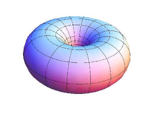
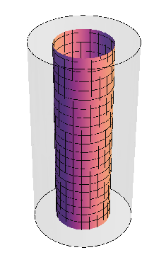
These surfaces represent a tube in $\mbox{AdS}_{3}$ and a torus in $\mbox{S}^{3}$ (see Fig. 1). Thus, the string is located around the ‘center’ of $\mbox{AdS}_{3}$ like a static particle in a rest frame. If one makes a boost transformation, string will oscillate around the center like a massive particle in AdS.

To understand the physical characteristics of the solutions (23), we introduce the conserved currents related to the isometry transformations (27). The Lie algebra valued currents in the $\mbox{SL}(2,\mathbb{R})$ sector are given by $L_{a}=\partial_{a}g\,g^{-1},\,\,$ $R_{a}=g^{-1}\,\partial_{a}g$ and inserting here the solution (23), we find

		$\displaystyle L_{\tau}=\lambda\,\hat{l}+\rho\,e^{\theta_{l}\,\hat{l}}\,g_{{}_{0}}\,\hat{r}\,g_{{}_{0}}^{-1}\,e^{-\theta_{l}\,\hat{l}}~,\quad$	$\displaystyle R_{\tau}=\lambda\,e^{-\theta_{r}\,\hat{r}}\,g_{{}_{0}}^{-1}\hat{l}\,g_{{}_{0}}\,e^{\theta_{r}\,\hat{r}}+\rho\,\hat{r}$
		$\displaystyle L_{\sigma}=\frac{m}{2}\,\hat{l}+\frac{n}{2}\,e^{\theta_{l}\,\hat{l}}\,g_{{}_{0}}\,\hat{r}\,g_{{}_{0}}^{-1}\,\epsilon^{-\theta_{l}\,\hat{l}}~,\quad$	$\displaystyle R_{\sigma}=\frac{m}{2}\,e^{-\theta_{r}\,\hat{r}}\,g_{{}_{0}}^{-1}\hat{l}\,g_{{}_{0}}\,e^{\theta_{r}\,\hat{r}}+\frac{n}{2}\,\hat{r}~.$

The equation of motion (15) for the $\mbox{SL}(2,\mathbb{R})$ part is equivalent to the current conservation law $\partial_{\tau}R_{\tau}-\partial_{\sigma}R_{\sigma}=0=\partial_{\tau}L_{\tau}-\partial_{\sigma}L_{\sigma}$, which is simply fulfilled by (25).

The induced metric tensor on the $\mbox{SL}(2,\mathbb{R})$ part can be written as

$$f_{ab}=\langle\,L_{a}\,L_{b}\,\rangle=\langle\,R_{a}\,R_{b}\,\rangle~,$$

(37)

and comparing it with (19) we obtain the equations

	$\displaystyle\lambda^{2}+\rho^{2}+2\lambda\,\rho\cosh 2\theta=\bar{\mu}^{2}+\mu^{2}+2\bar{\mu}\mu\cosh\alpha~,$
	$\displaystyle\frac{1}{4}(m^{2}+n^{2}+2mn\cosh 2\theta)=\bar{\mu}^{2}+\mu^{2}-2\bar{\mu}\mu\cosh\alpha~,$		(38)
	$\displaystyle\frac{1}{2}[\lambda m+\rho n+(\lambda n+\rho m)\cosh 2\theta]=\mu^{2}-\bar{\mu}^{2}~,$

which connect the parameters of the solution to the components of the induced metric tensor.

The $\mbox{SU}(2)$ conserved currents have the same form $L^{s}_{a}=\partial_{a}h\,h^{-1},\,\,$ $R^{s}_{a}=h^{-1}\,\partial_{a}h$ and from (19) and (23) we find the relations similar to (38)

	$\displaystyle\lambda_{s}^{2}+\rho_{s}^{2}+2\lambda_{s}\,\rho_{s}\cos 2\theta_{s}=\bar{\mu}^{2}+\mu^{2}+2\bar{\mu}\mu\cos\beta~,$
	$\displaystyle\frac{1}{4}(m_{s}^{2}+n_{s}^{2}+2m_{s}n_{s}\cos 2\theta_{s})=\bar{\mu}^{2}+\mu^{2}-2\bar{\mu}\mu\cos\beta~,$		(39)
	$\displaystyle\frac{1}{2}[\lambda_{s}m_{s}+\rho_{s}n_{s}+(\lambda_{s}n_{s}+\rho_{s}m_{s})\cos 2\theta_{s}]=\mu^{2}-\bar{\mu}^{2}~.$

The calculation of the $\mbox{SL}(2,\mathbb{R})$ conserved charges

$$L=\int_{0}^{2\pi}\frac{\mbox{d}\sigma}{2\pi}\,\,L_{\tau}~,\quad\quad R=\int_{0}^{2\pi}\frac{\mbox{d}\sigma}{2\pi}\,\,R_{\tau}~,$$

(40)

for the solution (23) yields (see Appendix)

$$L=(\lambda+\rho\,\cosh 2\theta)\,\hat{l}~,\quad\quad R=(\lambda\,\cosh 2\theta+\rho)\,\hat{r}~,$$

(41)

and, similarly, for the $\mbox{SU}(2)$ charges one gets

$$L_{s}=(\lambda_{s}+\rho_{s}\,\cos 2\theta_{s})\,\hat{l}_{s}~,\quad R_{s}=(\lambda_{s}\,\cos 2\theta_{s}+\rho_{s})\,\hat{r}_{s}~.$$

(42)

One can solve $\mu^{2}$ and $\bar{\mu}^{2}$ from the equations (38) and (39) separately and then comparing these solutions one finds two relations between the invariant parameters $\lambda$, $\rho$, $\theta$ and their spherical counterparts $\lambda_{s}$, $\rho_{s}$, $\theta_{s}$. Together with (25), we conclude that the space of isometrically invariant parameters is two dimensional. At this point we relate to each other the parameters of the $\mbox{AdS}_{3}$ and $\mbox{S}^{3}$ spaces. The joint analysis of the equations (38)-(39) for arbitrary $m$, $n$ and $m_{s}$, $n_{s}$ is rather complicated and, in general, they have no consistent solutions. In this paper we concentrate to the case $m_{s}=n_{s}=-m=n>0$. The corresponding $\mbox{AdS}_{3}$ and $\mbox{S}^{3}$ solutions (35) become

	$\displaystyle Y=\big(\cosh\theta\cos E\tau,~\cosh\theta\sin E\tau,~\sinh\theta\cos(F\tau-n\sigma),~\sinh\theta\sin(F\tau-n\sigma)\big)~,$
			(43)
	$\displaystyle X=\big(\sin\theta_{s}\,\sin A\tau,~\sin\theta_{s}\,\cos A\tau,~\cos\theta_{s}\,\sin(B\tau+n\sigma),~\cos\theta_{s}\,\cos(B\tau+n\sigma)\big)~,$

where $E=\lambda+\rho$, $F=\lambda-\rho$, $A=\lambda_{s}-\rho_{s}$ and $B=\lambda_{s}+\rho_{s}$. Due to (25), the new parameters are related by

$$F^{2}-E^{2}=n^{2}~,\qquad\qquad B^{2}-A^{2}=n^{2}~,$$

(44)

where $n$ is the winding number. For fixed $\tau$, the string (43) winds $n$-times around the circles in the $(Y^{1},\,Y^{2})$ and $(X^{3},X^{4})$ planes. Since the polar angle in the $\left(Y^{0^{\prime}},\,Y^{0}\right)$ plane corresponds to the time variable, the solution (43) describes string in a static gauge.

From eq. (38) we find

	$\displaystyle\mu^{2}=\frac{n^{2}}{4}\,(f-1)(f+\cosh 2\theta)~,\quad\bar{\mu}^{2}=\frac{n^{2}}{4}\,(f+1)(f-\cosh 2\theta)~,$
	$\displaystyle\cosh\alpha=\frac{e}{\sqrt{e^{2}-\sinh^{2}2\theta}}~,~~~~~~~~~~~~~~~~~~~~~~~~~~~$		(45)

where $e$ and $f$ are the rescaled variable $e=E/n$, $f=F/n$, with $f^{2}-e^{2}=1$. Eq. (39) similarly provides

	$\displaystyle\mu^{2}=\frac{n^{2}}{4}\,(b+1)(b+\cos 2\theta_{s})~,\quad\bar{\mu}^{2}=\frac{n^{2}}{4}\,(b-1)(b-\cos 2\theta_{s})~,$
	$\displaystyle\cos\beta=\frac{a}{\sqrt{a^{2}-\sin^{2}2\theta_{s}}}~,~~~~~~~~~~~~~~~~~~~~~~~~~~~$		(46)

with $a=A/n$ $b=B/n$, $b^{2}-a^{2}=1$. Choosing $b$ and $f$ as independent variables on the space of invariants, we find

$$\cosh 2\theta=bf-b^{2}+1~,\quad\quad\cos 2\theta_{s}=f^{2}-bf-1~.$$

(47)

Let us consider the parametrization of $g_{{}_{0}}$. It can be written as

$$g_{{}_{0}}=e^{\phi_{l}\,\hat{l}}\,e^{-(\gamma+\theta)\hat{n}}\,e^{\phi_{r}\,\hat{r}}~,$$

(48)

where $\hat{n}$ is a normalized commutator of the matrixes $\hat{l}$ and $\hat{r}$ (see (A.15)), $\gamma$ is the corresponding ‘angle’ variable between them and $\phi_{l}$, $\phi_{r}$ are arbitrary parameters. Eq. (48) has the following geometrical interpretation: $\hat{n}$ is a generator of boosts in the $(\hat{l},\hat{r})$ ‘plane’ (see (A.17)) and by (A.18) one finds the boost parameter $\alpha=\gamma+\theta$ to match (29). The angle parameters $\phi_{l}$ and $\phi_{r}$ in (48) then describe the freedom that leaves (29) invariant.

The parametrization of $h_{{}_{0}}$ is obtained in a similar way

$$h_{{}_{0}}=e^{\phi^{s}_{l}\,\hat{l}_{s}}\,e^{-(\gamma_{s}+\theta_{s})\hat{n}_{s}}\,e^{\phi^{s}_{r}\,\hat{r}_{s}}~,$$

(49)

where $n_{s},$ $\gamma_{s}$ and $\phi^{s}_{l}$, $\phi^{s}_{r}$ have the same geometrical interpretation in $\mbox{SU}(2)$ as their counterparts in $\mbox{SL}(2,\mathbb{R})$.

Now we recall that $(\tau,\,\sigma)$ coordinates still have a freedom in translations. Using equations (48), (49), and the form of the solutions (23), one can reduce the number of angle parameters ($\phi_{l}$, $\phi_{r},$ $\phi^{s}_{l}$, $\phi^{s}_{r}$) from four to two. We denote these two parameter by $\varphi_{1},$ $\varphi_{2}$. One can choose, for example, $\varphi_{1}=\phi_{l}=-\phi_{r}$ and $\varphi_{2}=\phi^{s}_{l}=\phi^{s}_{r}$.

Thus, solutions (23) are described by four unit vectors ($\hat{l}$, $\hat{r}$, $\hat{l}_{s}$, $\hat{r}_{s}$), two isometrically invariant parameters ($f$, $b$) and two remaining angle variables ($\varphi_{1},$ $\varphi_{2}$). Totally, one gets twelve dimensional space of parameters.

To find the Poisson bracket structure on this space, one can calculate the symplectic form of the system $\omega=\mbox{d}\vartheta$ on the space of solutions (23) and invert it. The presymplectic 1-form $\vartheta$ is defined from the string Lagrangian in the first order formalism

$$\vartheta=\int_{0}^{2\pi}\frac{\mbox{d}\sigma}{2\pi}\,\left[\langle R\,g^{-1}\,\mbox{d}g\rangle+\langle R_{s}\,h^{-1}\,\mbox{d}h\rangle\right]~.$$

(50)

Here $R$ and $R_{s}$ are Lie algebra valued variables, which in the conformal gauge are associated with $g^{-1}\partial_{\tau}g$ and $h^{-1}\partial_{\tau}h$, respectively. Before we discuss the reduction of the symplectic form on the string solutions, let us consider particle dynamics in $\mbox{SL}(2,\mathbb{R})\times\mbox{SU}(2)$ and compare it to our system.

Particle trajectories in the $\mbox{SL}(2,\mathbb{R})$ sector are parameterized either by a pair ($g_{{}_{0}},\,R$) or ($g_{{}_{0}},\,L$)

$$g(\tau)=e^{L\,\tau}\,g_{{}_{0}}=g_{{}_{0}}\,e^{R\,\tau}~,$$

(51)

where $R$ and $L$ are the dynamical integrals for the isometry transformations.²² 2 We use same notations as for string solutions. They are related to each other by the adjoint transformation

$$g\,R\,g^{-1}=L~,$$

(52)

and, therefore, they are on the same coadjoint orbit.

The description of $\mbox{SU}(2)$ sector is similar and the orbits in both cases are defined by the Casimir numbers

$$\langle\,L\,L\,\rangle=\langle\,R\,R\,\rangle=-m^{2}~,\quad\quad\langle\,L_{s}\,L_{s}\,\rangle=\langle\,R_{s}\,R_{s}\,\rangle=m_{s}^{2}~.$$

(53)

These numbers are related to the particle mass $M$ by the massshell condition

$$m^{2}-m_{s}^{2}=M^{2}~,$$

(54)

and the dynamical integrals can be written as

$$L=m\,\hat{l}~,\quad\quad R=m\,\hat{r}~;\quad\quad L_{s}=m_{s}\,\hat{l}_{s}~,\quad\quad\quad R_{s}=m_{s}\,\hat{r}_{s}~,$$

(55)

where $\hat{l},$ $\hat{r}$ and $\hat{l}_{s},$ $\hat{r}_{s}$ are unit vectors as for the string solutions (see (41)-(42)).

Hamiltonian formulation can be started in $(R,\,g)$, $(R_{s},\,h)$ variables and the presymplectic 1-form $\vartheta=\langle R\,g^{-1}\,\mbox{d}g\,\rangle+\langle R_{s}\,h^{-1}\,\mbox{d}h\,\rangle$, as in (50). However, in order to make further comparison with the string solutions, it is more convenient to use left and right dynamical integrals symmetrically and express $g$ and $h$ through them.

Let us consider the $\mbox{SL}(2,\mathbb{R})$ part. One can show that eq. (52) defines $g$ up to an angle variable $\varphi$ [11]

$$g=e^{\theta_{{}_{L}}\,\hat{n}_{{}_{L}}}\,e^{\varphi\,{\bf t}_{0}}\,e^{\theta_{{}_{R}}\,\hat{n}_{{}_{R}}}~.$$

(56)

Here

$$\hat{n}_{{}_{L}}=\frac{[{\bf t}_{0},\,\hat{l}]}{2\sinh 2\theta_{{}_{L}}}~,\quad\quad\hat{n}_{{}_{R}}=-\frac{[{\bf t}_{0},\,\hat{r}]}{2\sinh 2\theta_{{}_{R}}}~$$

(57)

are normalized vectors and $\cosh 2\theta_{{}_{L}}=-\langle\,\hat{l}\,{\bf t}_{0}\,\rangle,\,$ $\,\cosh 2\theta_{{}_{R}}=-\langle\,\hat{r}\,{\bf t}_{0}\,\rangle$ (see Appendix).

The symplectic form of the AdS part $\omega_{{}_{AdS}}=\mbox{d}\langle R\,g^{-1}\,\mbox{d}g\rangle$ calculated in the coordinates $(\hat{l},\hat{r},m,\varphi)$ splits into the sum of three terms

$$\omega_{{}_{AdS}}=m\,\omega_{{}_{L}}+m\,\omega_{{}_{R}}-\mbox{d}m\wedge\mbox{d}\varphi~,$$

(58)

where

$$\omega_{{}_{L}}=\frac{\mbox{d}l_{2}\wedge\mbox{d}l_{1}}{2l^{0}}~,\quad\quad\omega_{{}_{R}}=\frac{\mbox{d}r_{1}\wedge\mbox{d}r_{2}}{2r^{0}}$$

(59)

are the symplectic forms on the unit $\mbox{SL}(2,\mathbb{R})$ coadjoint orbits expressed in terms of the vector components $l_{\mu}=\langle\,{\bf t}_{\mu}\,\hat{l}\,\rangle$ and $r_{\mu}=\langle\,{\bf t}_{\mu}\,\hat{r}\,\rangle$.

The $\mbox{SU}(2)$ part of the symplectic form has a similar structure

$$\omega_{s}=m_{s}\,\omega_{{}_{L}}^{s}+m_{s}\,\omega_{{}_{R}}^{s}+\mbox{d}m_{s}\wedge\mbox{d}\varphi_{s},$$

(60)

where now $\omega_{{}_{L}}^{s}$ and $\omega_{{}_{R}}^{s}$ are symplectic forms on the unit $\mbox{SU}(2)$ coadjoint orbits.

References

• [1] J. M. Maldacena, “The large N limit of superconformal field theories and supergravity,” Adv. Theor. Math. Phys. 2 (1998) 231 [Int. J. Theor. Phys. 38 (1999) 1113] [arXiv:hep-th/9711200].
• [2] D. E. Berenstein, J. M. Maldacena and H. S. Nastase, “Strings in flat space and pp waves from N = 4 super Yang Mills,” JHEP 0204 (2002) 013 [arXiv:hep-th/0202021].
• [3] J. A. Minahan and K. Zarembo, “The Bethe-ansatz for N = 4 super Yang-Mills,” JHEP 0303 (2003) 013 [arXiv:hep-th/0212208].
• [4] I. Bena, J. Polchinski and R. Roiban, “Hidden symmetries of the A​d​S​(5)×S5AdS(5)\times S^{5} superstring,” Phys. Rev. D 69, 046002 (2004) [hep-th/0305116].
• [5] N. Beisert, C. Ahn, L. F. Alday, Z. Bajnok, J. M. Drummond, L. Freyhult, N. Gromov and R. A. Janik et al., “Review of AdS/CFT Integrability: An Overview,” Lett. Math. Phys. 99, 3 (2012) [arXiv:1012.3982 [hep-th]].
• [6] H. Dorn, N. Drukker, G. Jorjadze and C. Kalousios, “Space-like minimal surfaces in A​d​S×SAdS\times S,” [arXiv:0912.3829 [hep-th]].
• [7] H. Dorn, G. Jorjadze, C. Kalousios, L. Megrelidze and S. Wuttke, “Vacuum type space-like string surfaces in A​d​S3×S3AdS_{3}\times S^{3},” J. Phys. A A 44, 025403 (2011) [arXiv:1007.1204 [hep-th]].
• [8] L. F. Alday and J. M. Maldacena, “Gluon scattering amplitudes at strong coupling,” JHEP 0706, 064 (2007) [arXiv:0705.0303 [hep-th]].
• [9] L. F. Alday and J. Maldacena, “Comments on gluon scattering amplitudes via AdS/CFT,” JHEP 0711 (2007) 068 [arXiv:0710.1060 [hep-th]]. L. F. Alday, “Lectures on Scattering Amplitudes via AdS/CFT,” Fortsch. Phys. 56, 816 (2008) [arXiv:0804.0951 [hep-th]]. L. F. Alday and J. Maldacena, “Null polygonal Wilson loops and minimal surfaces in Anti-de-Sitter space,” JHEP 0911 (2009) 082 [arXiv:0904.0663 [hep-th]]. L. F. Alday, D. Gaiotto and J. Maldacena, “Thermodynamic Bubble Ansatz,” [arXiv:0911.4708 [hep-th]]. L. F. Alday, J. Maldacena, A. Sever and P. Vieira, “Y-system for Scattering Amplitudes,” [arXiv:1002.2459 [hep-th]].
• [10] K. Pohlmeyer, “Integrable Hamiltonian Systems And Interactions Through Quadratic Constraints,” Commun. Math. Phys. 46 (1976) 207. H. J. De Vega and N. G. Sanchez, “Exact Integrability Of Strings In D-Dimensional De Sitter Space-Time,” Phys. Rev. D 47 (1993) 3394. M. Grigoriev and A. A. Tseytlin, “Pohlmeyer reduction of AdS5×S5\mbox{AdS}_{5}\times S^{5} superstring sigma model,” Nucl. Phys. B 800 (2008) 450 [arXiv:0711.0155 [hep-th]]. A. Jevicki, K. Jin, C. Kalousios and A. Volovich, “Generating AdS String Solutions,” JHEP 0803 (2008) 032 [arXiv:0712.1193 [hep-th]]. H. Dorn, G. Jorjadze and S. Wuttke, “On space-like and time-like minimal surfaces in AdSn\mbox{AdS}_{n},” JHEP 0905 (2009) 048 [arXiv:0903.0977 [hep-th]].
• [11] G. Jorjadze, L. O’Raifeartaigh and I. Tsutsui, “Quantization of a relativistic particle on the SL(2,R) manifold based on Hamiltonian reduction,” Phys. Lett. B 336, 388 (1994) [hep-th/9407059].
• [12] H. Dorn, G. Jorjadze, C. Kalousios and J. Plefka, “Coordinate representation of particle dynamics in AdS and in generic static spacetimes,” J. Phys. A A 44, 095402 (2011) [arXiv:1011.3416 [hep-th]]. F. Passerini, J. Plefka, G. W. Semenoff and D. Young, “On the Spectrum of the A​d​S5×S5AdS_{5}\times S^{5} String at large lambda,” JHEP 1103, 046 (2011) [arXiv:1012.4471 [hep-th]].