Shell Models of Magnetohydrodynamic Turbulence
Abstract
Shell models of hydrodynamic turbulence originated in the seventies. Their main aim was to describe the statistics of homogeneous and isotropic turbulence in spectral space, using a simple set of ordinary differential equations. In the eighties, shell models of magnetohydrodynamic (MHD) turbulence emerged based on the same principles as their hydrodynamic counter-part but also incorporating interactions between magnetic and velocity fields. In recent years, significant improvements have been made such as the inclusion of non-local interactions and appropriate definitions for helicities. Though shell models cannot account for the spatial complexity of MHD turbulence, their dynamics are not over simplified and do reflect those of real MHD turbulence including intermittency or chaotic reversals of large-scale modes. Furthermore, these models use realistic values for dimensionless parameters (high kinetic and magnetic Reynolds numbers, low or high magnetic Prandtl number) allowing extended inertial range and accurate dissipation rate. Using modern computers it is difficult to attain an inertial range of three decades with direct numerical simulations, whereas eight are possible using shell models.
In this review we set up a general mathematical framework allowing the description of any MHD shell model. The variety of the latter, with their advantages and weaknesses, is introduced. Finally we consider a number of applications, dealing with free-decaying MHD turbulence, dynamo action, Alfvén waves and the Hall effect.
| Variables | , , , , a, , |
|---|---|
| External magnetic field, forcing, vorticity | , f, |
| Wave numbers | k, p, q |
| Energies, helicities, enstrophy, squared magnetic potential | , , , , , , |
| Complex conjugation, complex conjugate of | , |
| Dimensionless numbers | , , , |
| Viscosity, diffusivity, density | , , |
| Injection rate of energy, kinetic helicity, cross helicity, magnetic helicity | , , , |
| Viscous, Joule dissipation rate | , |
| Rotation rate, Alfvén wave velocity | , |
| Characteristic time scales | , , , , |
| Characteristic length scales | , |
| Characteristic velocity and magnetic fluctuations at scale | |
| Velocity and magnetic structure functions, scaling exponent | |
| Specific wave number modulus | , , , , |
| Shell common ratio | |
| Kinematic growthrate | |
| Shell variables | , , , , |
| Shell wave number, forcing | , |
| Quadratic functions | |
| Quadratic quantities in shell | , , , , , |
| Energy transfer | |
| Energy flux | |
| Mode-to-mode energy transfer | |
| Non-locality parameter |
1 Introduction
In astrophysical objects most fluids are electrically conducting and generally exhibit highly turbulent motion due to the large dimensions involved (Schekochihin and Cowley, 2007). Such magnetohydrodynamic (MHD) turbulence is at the heart of the dynamo action generating magnetic fields in planets, stars and galaxies (Brandenburg and Subramanian, 2005; Tobias et al., 2011). Dynamo action has been the object of several experiments (Gailitis et al., 2000; Stieglitz and Müller, 2001; Shew and Lathrop, 2005; Monchaux et al., 2007; Spence et al., 2007; Nataf et al., 2008; Frick et al., 2010) and is suspected to occur in nuclear reactors cooled with liquid sodium (Plunian et al., 1999). MHD turbulence is also responsible for the propagation of Alfvén waves (Alfvén, 1942) in the presence of an external magnetic field as in e.g. the solar wind. Such waves can be reproduced in MHD experiments (Alboussière et al., 2011) and measured in plasma tokamaks (Gekelman, 1999). Complementary to observation and experiment, direct numerical simulations aimed at reproducing the finest details of MHD turbulence have been performed (Müller et al., 2003). However, one serious difficulty faced by simulations is that the processes involved are strongly non-linear implying, for example, that the energy is transferred over an extended range of scales (Verma, 2004). This range is several orders of magnitude larger than what is attainable with present day or, indeed, projected computers. In this respect shell models are of primary importance in building up our understanding. First introduced to deal with hydrodynamic (HD) turbulence, shell models have now been generalized to MHD, leading to interlocked progresses of both types of model. We will now summarize the evolution of these ideas.
Obukhov (1971) introduced a multilevel system of non-linear triplets to mimic the energy transport, in the spirit of the Richardson-Kolmogorov scenario for the energy cascade in HD turbulence. This idea has been successfully developed by his team (Gledzer, 1973; Desnianskii and Novikov, 1974; Glukhovskii, 1975; Gledzer et al., 1981). At the same time Lorenz (1971) started from the full Fourier representation of the Navier-Stokes equations. Aiming at studying the statistical properties of turbulent flow with limited computer facilities, he reduced the set of equations to a “very low order model". Though both approaches were different, Lorenz (1972) and Gledzer (1973) eventually derived the same shell model of HD turbulence 11 1 First denoted “cascade” or “scalar” models, such models have been called “shell” in the beginning of the nineties.. They both applied the conservation of kinetic energy and enstrophy with the description of atmospheric turbulence statistics in mind. We note that these two quantities, kinetic energy and enstrophy, are positive definite and so are rather straightforward to define in the framework of shell models, explaining why shell models of 2D-turbulence were preferred at that time. It took a further 20 years (Kadanoff et al., 1995) to identify and adequately describe kinetic helicity (not sign definite) in shell models, leading to 3D-turbulence modeling (for which kinetic helicity, instead of enstrophy, is ideally conserved).
Other low order models of turbulence appearing in the seventies were all based on the same principle: the division of isotropic spectral space into a set of concentric shells using only one variable per shell to characterize velocity fluctuations. The main difference between the models were the degree of locality between two interacting shells, each shell interacting either with one first neighbor (Obukhov, 1971; Desnianskii and Novikov, 1974; Bell and Nelkin, 1978; Kerr and Siggia, 1978) - with only one quadratic invariant (kinetic energy) - or two first neighbors (Lorenz, 1972; Gledzer, 1973; Glukhovskii, 1975; Gledzer and Makarov, 1979) - with two quadratic invariants (kinetic energy and enstrophy).
In the next decade, Zimin (1981) introduced the so-called ‘‘hierarchical model of turbulence" with self-similar functions localized in both physical and Fourier spaces 22 2 In terms of contemporary scientific language, these functions would be called wavelets, as discussed by Frick and Zimin (1993).. Projecting the Navier-Stokes equations on this base of functions, he obtained a set of ordinary differential equations organized in a hierarchical tree. By reducing this hierarchical tree to one vertical chain, Frik (1983) 33 3 In papers, translated from Russian journals, Peter Frick was spelt as Frik P.G. and we keep each time the spelling from the cited paper. constructed a shell model for 2D-turbulence - with two quadratic invariants (kinetic energy and enstrophy) - including not only local interactions as in Lorenz (1972) and Gledzer (1973) but also non-local interactions.
From the very first numerical simulations of the shell model equations, it was clear that the Kolmogorov solution (or Kraichnan’s in 2D) gave an unstable fixed point, and that a Kolmogorov spectrum of energy could be obtained only by averaging over time, as expected in real turbulence. However, such models failed to show any chaotic behavior. The link to intermittency was still missing, until the first MHD shell models were derived (Frik, 1984; Gloaguen et al., 1985). Indeed, by doubling the degrees of freedom (adding the magnetic field), chaotic behavior was obtained. A similar effect had also been observed with temperature in shell models of convective turbulence (Frik, 1986; Frik, 1987). Applying this idea to HD turbulence, Yamada and Ohkitani (1987); Yamada and Ohkitani (1988) used a velocity with two real components instead of only one, and obtained solutions showing chaotic behavior. With such complex velocity they found intermittency statistics in excellent agreement with real HD turbulence.
In the following years such models of HD turbulence aroused wide interest (Pisarenko et al., 1993; Carbone, 1994b; Biferale et al., 1995; Kadanoff et al., 1995; Frick et al., 1995). A spurious regularity in the spectral properties (a three-shell periodicity) identified by Biferale (1993) was corrected either by using a slightly different model (L’vov et al., 1998) or by considering a velocity with three real components per shell instead of two (Aurell et al., 1994a).
After the identification of kinetic helicity by Kadanoff et al. (1995), the first model of 3D MHD turbulence was derived (Brandenburg et al., 1996; Basu et al., 1998; Frick and Sokoloff, 1998) with total energy, magnetic and cross helicities as quadratic invariants. Meanwhile, new shell models for HD turbulence were elaborated in which the velocity is projected onto helical modes (Zimin and Hussain, 1995; Benzi et al., 1996b). In such helical models the helicity is not correlated with the kinetic energy, contrary to the other models. This gives rise to important differences when dealing with kinetic helicity in HD turbulence (Stepanov et al., 2009; Lessinnes et al., 2011). It is also suitable to study magnetic and cross helicities in MHD turbulence (Frick and Stepanov, 2010).
Within the last ten years more complex shell models have been elaborated to account for characteristics peculiar to MHD turbulence. These models include non-local interactions, directly within triads (Plunian and Stepanov, 2007) or with the help of multi-scale models (Frick et al., 2006), anisotropy (Nigro et al., 2004), and the Hall effect (Frick et al., 2003).
Our review is organized as follows. After a short description of MHD turbulence in Sec. 2, a general framework is introduced in Sec. 3 providing a description of various shell models derived so far. This is followed in Sec. 4 by a review of results obtained for different applications. For the sake of clarity, HD shell models will often be introduced before MHD shell models. However, we will focus on MHD applications only. For HD applications the reader can refer to reviews by e.g. Bohr et al. (1998), Biferale (2003), Frick (2003), Ditlevsen (2011). A list of notations that are used in the review is given in Table 1.
2 MHD turbulence
In this section we simply review some background information necessary to address the next sections. For deeper knowledge the reader can refer to reference books on HD (Frisch, 1995; Lesieur, 1997) and MHD (Moreau, 1990; Davidson, 2001; Biskamp, 2003) turbulence.
2.1 Physical space
2.1.1 MHD equations
The incompressible MHD equations that govern the time evolution of the velocity and the magnetic induction are
| (1) | |||||
| (2) |
where is the viscosity, the magnetic diffusivity, the total pressure (including the magnetic pressure) and f the flow forcing, normalized by the fluid density . These equations are derived from the Navier-Stokes equations supplemented by the Lorentz force, and Maxwell equations for which advantage has been taken of fast charge redistribution commonly found in liquid metals. The magnetic induction has been normalized by such that is given in units of velocity. Here we are interested only in fluctuation, assuming that and average to zero in space and time.
The non-linear terms on the r.h.s. (right hand side) redistribute kinetic and magnetic energies among the full range of scales from the largest, defined by the system boundaries, to the smallest at which the total energy dissipates. Different kinds of helicities are also transferred. Such transfers are called direct or inverse, depending on whether they occur towards smaller or larger scales. They are also described as local or non-local depending on whether they occur between neighboring scales or not.
We speak of forced or decaying turbulence depending on whether f is different from or equal to zero and dynamo action when the magnetic energy does not decay in time, meaning that the energy transfer from kinetic to magnetic is sufficient to compensate for the magnetic dissipation.
In the presence of an external magnetic field (having a velocity dimension as it is normalized by ), Eqs. (1-2) can be rewritten by replacing by . Introducing the so-called Elsässer variables defined as
| (3) |
the MHD equations become
| (4) |
where and is assumed to be independent of space coordinates. Provided is sufficiently strong, Eq. (4) can be linearized and thus becomes a wave equation the solutions of which are the so-called Alfvén waves (Alfvén, 1942). This set of equations is only symmetric for . Taking has the effect of suppressing the reflection of Alfvén waves at the walls (Schaeffer et al., 2011).
2.1.2 Quadratic invariants
In MHD three integral quantities play a special role: the total energy, the cross helicity and the magnetic helicity. The total energy, , is the sum of the kinetic energy and the magnetic energy ,
| (5) |
where is the volume of integration. The cross helicity and magnetic helicity are defined as
| (6) |
where a is the vector potential satisfying .
The absolute value of cross helicity is maximal if and are aligned (and zero if they are perpendicular).
The quadratic quantities and are called invariant because in the ideal limit of a non-viscous and non-diffusive fluid , and in the absence of forcing and an external magnetic field (), they are conserved in time,
| (7) |
The first two conservation laws can be shown from Eqs. (1-2) provided appropriate boundary conditions are used while the third conservation law is obtained from Eq. (2). We can also show that the first two conservation laws are equivalent using the following property
| (8) |
which is satisfied for any divergence-free vectors x and y. Then the conservation of total energy and cross helicity take the following forms
| (9) | |||||
| (10) |
Exchanging and does not change and . However, Eqs. (9) and (10) are exchanged, showing the equivalence of the two conservation laws.
We note that the kinetic helicity, defined by
| (11) |
where is the vorticity, is not conserved in MHD. Hence
| (12) |
indicating that kinetic helicity can be created or suppressed by the interaction between the vorticity and the magnetic field. For the kinetic energy and helicity are conserved. In the presence of an external magnetic field , the magnetic helicity is not conserved anymore.
Finally, in 2D HD turbulence the kinetic helicity is always zero. Instead enstrophy
| (13) |
is conserved along with the kinetic energy.
In 2D MHD turbulence magnetic helicity is always constant. Instead the square potential
| (14) |
is conserved together with the total energy and cross helicity.
2.1.3 Dimensionless parameters
The Reynolds number is defined as
| (15) |
where is a characteristic velocity and is a characteristic scale. Putting in Eq. (1), shows how strong the non-linear interactions are, compared with viscous dissipation.
In MHD the magnetic Reynolds number is defined as
| (16) |
From Eq. (2) shows how strong the non-linear interactions are, compared with magnetic dissipation.
The ratio of both numbers is called the magnetic Prandtl number
| (17) |
and depends only on the fluid properties. The dimensionless form of Eqs. (1-2) is obtained by replacing and by and respectively.
Fully developed turbulence implies high (greater than at the largest scale). Dynamo action requires at the scale where the magnetic energy grows. This corresponds to typical of to when is calculated at the largest scale of the system. The latter condition is difficult to meet experimentally with liquid metals. Indeed the power necessary to run a liquid metal experiment increases as (Pétrélis and Fauve, 2001), demanding a considerable effort to reach at the largest scale. Liquid sodium is usually used for its high conductivity, and for its density about unity. With , reaching would require .
In Fig. 1 a few typical objects are placed on the map (,). Among them liquid metal experiments, fast breeder reactors, the Earth’s core, Jupiter’s core and the Sun’s convective zone correspond to to . We note that such low values for and also realistic values remain beyond the limits of current direct numerical simulations (Sakuraba and Roberts, 2009; Uritsky et al., 2010).

2.1.4 Homogeneity and isotropy
Two assumptions are usually made in order to obtain theoretical predictions for both HD and MHD turbulence. The first assumes homogeneity, meaning that the statistical quantities derived from the flow and magnetic fields are invariant under translation in physical space. This assumption fails to predict, for example, the effect of boundary layers. The second assumes isotropy, meaning that the statistical quantities are independent of direction. In principle isotropy is broken as soon as a sufficiently strong external magnetic field or rotation is applied.
Most 3D shell models are based upon this double assumption of homogeneity and isotropy. However, several models have been developed to relax the assumption of isotropy in the context of Alfvén waves (see Sec 4.4.2).
2.1.5 Isotropic phenomenology
In his paper Kolmogorov (1941) introduced the structure function for the velocity field
| (18) |
where is the longitudinal velocity increment
| (19) |
and denotes ensemble averaging. In HD turbulence, the power which drives the flow at forcing scale , is transferred towards smaller scales and, in a stationary state, is equal to the energy dissipation rate (Kolmogorov, 1941; Obukhov, 1941). This direct energy cascade occurs within the inertial range corresponding to scales such that , where is the viscous scale below which viscous dissipation dominates. In such an inertial range, assuming isotropy, a simple dimensional analysis leads to the estimation
| (20) |
This corresponds to an energy transfer rate , where is the eddy turn-over time. Then for any ,
| (21) |
The viscous scale is estimated by assuming that the power , which is injected into the fluid at some forcing scale, is subsequently dissipated by viscosity at scale , corresponding to . This leads to
| (22) |
In MHD turbulence at high , the estimate of depends on . For applying the same type of phenomenology as above for and , we estimate the viscous and ohmic scales to be
| (23) |
where and are the fractions of that correspond to the viscous and the ohmic dissipation respectively () . The ratio of these two scales is
| (24) |
For , assuming that the magnetic energy is produced by the velocity shear which is maximum at scale , the scale at which the magnetic energy dissipates is given by , leading to
| (25) |
This immediately shows the difference between low- MHD turbulence, as in liquid metal, high- MHD turbulence, as in interstellar medium, and , as in direct numerical calculations. For magnetic energy dissipation occurs at a much larger scale than that of the kinetic energy, and vice-versa for . For , an example is given in Fig.2, both kinetic and magnetic energies dissipate at about the same scale.
The ratio , about which little is known, depends on the level of the magnetic energy compared to the level of the kinetic energy. In general we have in experiments and in real astrophysical objects. In MHD shell models, for , leading to (Plunian and Stepanov, 2010).
The structure functions for the magnetic field are defined similarly to Eq. (18), as
| (26) |
Assuming a Kolmogorov scaling law, given by Eq. (20), for both magnetic and velocity fields leads to the same scaling for both structure functions .
In the presence of an external magnetic field , a different mechanism of energy transfer occurs due to the interaction of Alfvén waves (Iroshnikov, 1964; Kraichnan, 1965). Indeed, such an applied field leads to an additional time scale . Provided is sufficiently strong, can be shorter than the eddy turnover time . Then energy transfer occurs on the Alfvén time scale, leading to
| (27) |
and onto
| (28) |
Deviation from isotropy leads to other time scales and scaling laws (see Sec. 2.2.3).
2.1.6 Intermittency
If structure functions obtained from HD experimental measurements exhibit clear scaling laws, their slopes, however, clearly deviate from as is increased. This is interpreted as the signature of intermittent events, like bursts, which are not captured by the self-similarity assumption of the Kolmogorov (1941) theory. Such intermittency is quantified by the scaling exponent such that
| (29) |
Various models of intermittency have been proposed aiming at an analytical formula for the scaling exponent (Frisch, 1995). Here we draw attention to the elegant parameter-free formula of She and Leveque (1994)
| (30) |
which gives , consistent with the Kolmogorov “4/5" law.
It is based on
(i) the Kolmogorov refined similarity hypothesis:
where is the energy dissipation averaged over a volume ,
(ii) log-Poisson statistics for the dissipation rate fluctuations,
(iii) one-dimensional (filament-like) form of the ultimate dissipative structures.
The scaling exponent given by Eq. (30) is in excellent agreement with experimental measurements of isotropic HD turbulence.
There is, however, good reason to expect that Eq. (30) is not valid in MHD turbulence, even if both magnetic and velocity fields satisfy the same Kolmogorov scaling law given by Eq. (20).
The difference comes from the different nature of the ultimate dissipative structures, which might be sheet-like rather than filament-like. Thus, after replacing hypothesis (iii) of She-Leveque by
(iv) the ultimate dissipative structure is two-dimensional (sheet-like),
Horbury and Balogh (1997) and Müller and Biskamp (2000) proposed a MHD version of Eq. (30)
for
| (31) |
which again gives .
When applied to Alfvén wave turbulence not only must (iii) be replaced by (iv), but (i) must also be replaced by the Iroshnikov-Kraichan relation
(v) .
Subsequently Grauer et al. (1994) and Politano and Pouquet (1995) developed the Alfvénic version of Eq. (30)
| (32) |
with .
In experiments and/or numerical simulations, accurate measurements of scaling exponents are needed in order to discriminate between the three formulas given above by Eqs. (30-32). When dealing with high order structure functions, which is necessary for discrimination, it is even hard to identify the appropriate range of scales which can be used for the determination of the scaling laws. In this respect, significant progress has been made by Benzi et al. (1993b) who discovered the concept of Extended Self-Similarity (ESS) while calculating high order structure functions from wind tunnel experimental results. The ESS takes advantage of the Kolmogorov “4/5" law
| (33) |
so providing an exact linear relation between the third order structure function and the scale within the inertial range. Instead of plotting the structure function versus , leading to a power scaling , they plotted versus . As expected they found that the power scaled as . Furthermore, they discovered that this scaling held for a range of scales much larger (both in small and large scale directions) than that for which holds. Benzi et al. (1993b) therefore claimed an extended self-similarity range of scales. In addition, they found that by using this method the accuracy in the estimate of the scaling exponents was much improved. ESS was tested and used for the measurement of scaling exponents in a variety of turbulent flow conditions, including MHD turbulence (Rowlands et al., 2005).
2.2 Fourier space
2.2.1 Triads
Assuming triply periodic boundary conditions in a cube of volume , both fields, flow and induction, can be expanded into discrete Fourier series:
| (34) |
where and are the complex Fourier coefficients defined as
| (35) |
The conditions and must be satisfied in order that and be real vectors. In Fourier space the divergence-free form of both and is given by
| (36) |
indicating that both fields are perpendicular to k. Similarly, both Navier-Stokes and induction equations can be projected onto a plane perpendicular to k in Fourier space, making it possible to remove the pressure terms without loss of generality. These equations are (Biskamp, 2003)
| (37) | |||||
| (38) |
where is the operator defined by the matrix and corresponds to the projection of x on the plane perpendicular to k. Only the subset of wave numbers k, p and q satisfying , interact together. Such a triad is illustrated in Fig. 5.
It can be shown that all the quadratic invariants introduced above are also conserved within each triad. Hence we can define energy and helicity transfer only between three modes belonging to the same triad. The formalism for mode-to-mode energy transfer in MHD turbulence has been developed in detail by Verma (2004) and can be generalized to helicity (cross or magnetic) transfer. This formalism will be transposed to shell models in Sec. 3.
2.2.2 Spectra
The Fourier spectra of the quadratic quantities introduced in Sec. 2.1.2 are
| (39) | |||||
| (40) | |||||
| (41) | |||||
| (42) | |||||
| (43) |
where means the complex conjugate. Their power density spectra are defined in their integral form
| (44) |
or discrete form
| (45) |
where denotes any of the above quadratic quantities. In addition the following conditions are satisfied (Frisch et al., 1975)
| (46) |
Of course all these quantities depend strongly on time. However, we can look for states which are statistically stationary or at least with a time dependency much larger than that of the time scale of the fluctuations (e.g. in free-decaying turbulence). Not only energies but also helicities are expected to cascade. From absolute equilibrium distributions, which depend only on the quadratic invariants, Frisch et al. (1975) found that the cascade is direct for the total energy and cross helicity, and inverse for the magnetic helicity. This makes a striking difference with the HD case for which, using the same method, Kraichnan (1973) found that both the kinetic energy and helicity cascades are direct. The results also depend on whether the MHD turbulence is forced or freely decaying , with or without the presence of an external magnetic field .

An example of forced MHD dynamo turbulence for is given in Fig. 2. From dimensional arguments, if the velocity and magnetic field increments satisfy , then the corresponding spectral energy densities satisfy . Assuming , this leads to the famous “-5/3" Kolmogorov scaling law
| (47) |
for both kinetic and magnetic energy density spectra. HD turbulence experiments clearly demonstrate the existence of such a scaling law over more than three decades (Saddoughi and Veeravalli, 1994; Pope, 2000). This is also observed in DNS over more than one decade (Gotoh et al., 2002). In MHD turbulence there is, however, not such a clear inertial range for the magnetic energy density spectrum, as depicted in Fig. 2. Even the kinetic energy inertial range is rather short, less than one decade in Fig. 2, making it difficult to identify a clear scaling law. Short spectra are due to limited numerical resolution. Presumably future higher resolution will give rise to wider inertial range. The shape of the magnetic spectrum also depends on forcing. In particular if the forcing is helical the spectrum can be peaked at the largest possible scale (Brandenburg, 2001; Brandenburg, 2009). Such large-scale magnetic field generation by the small-scale MHD turbulence corresponds to the so-called -effect (Krause and Rädler, 1980). For free-decaying MHD turbulence and Müller and Biskamp (2000) and Müller and Grappin (2005) found clear Kolmogorov scaling laws.
2.2.3 Spectra in presence of an external magnetic field


As mentioned in Sec. 2.1.5, the presence of an external magnetic field changes the energy transfer which occurs at the Alfvén time scale rather than at the eddy turn-over time scale , provided is strong enough. Assuming isotropy, the following spectra are expected (Iroshnikov, 1964; Kraichnan, 1965)
| (48) |
Unfortunately, in MHD turbulence experiments (Odier et al., 1998; Alemany et al., 2000; Bayliss et al., 2007) the values of which are possible to achieve are too low (less than 10 at the largest scale) to observe a sufficiently wide magnetic inertial range. In the left panel of Fig. 3, a typical magnetic energy density spectrum is plotted versus frequency (Bourgoin et al., 2002). Two slopes are observed, -1 and -11/3, neither of which can be attributed to an inertial range. The first slope is not easy to understand. On the other hand the second slope can be justified as follows (Golitsyn, 1960; Moffatt, 1961). First we have to assume that the Taylor hypothesis applies in order to interpret the frequency as a wave number. The induction equation (2), replacing by , where is taken to be independent of any spatial coordinate, and assuming (low ), implies
| (49) |
In a stationary statistic state the induction term is balanced by the dissipation term , implying . Now assuming that the turbulent velocity obeys the Kolmogorov scaling law (20), we find
| (50) |
Applying Taylor hypothesis, Eq. (50) implies that . We note that such line of argument assumes non-local interactions between the applied field and the small-scale turbulence.
If the IK scaling law (48) cannot be tested against experiments, at least it can be compared with observations. The right panel of Fig. 3 shows the magnetic energy density spectrum measured in the solar wind. The corresponding MHD turbulence subjected to the strong magnetic field emanating from the Sun, shows three successive slopes, again at large scales, in the inertial range, and at the smallest scales. An interesting point here is that an inertial Kolmogorov scaling law is obtained instead of the IK scaling law (for a discussion of the two other slopes see e.g. Verdini et al. (2012a) and Howes et al. (2011)).
In fact anisotropy plays a crucial role in Alfvén wave turbulence (Goldreich and Sridhar, 1995), leading to modified definitions for both the Alfvén time and the eddy turn-over time , where the subscripts and denote the directions parallel and perpendicular to the applied field . Two regimes are possible, depending whether or . They are denoted by weak and strong turbulent regimes respectively. In the weak regime, on the basis of resonant three-wave interactions, Galtier et al. (2000) found a cascade restricted to the perpendicular plane, with . This has been numerically confirmed (Boldyrev and Perez, 2009). In the strong regime the cascade occurs in both perpendicular and parallel directions. Provided the critical balance is satisfied, the magnetic energy spectrum is now expected to satisfy and (Goldreich and Sridhar, 1995). This seems to be well supported by solar wind measurements (Horbury et al., 2008), but still lacks numerical confirmation. Instead simulations give an energy spectrum (Müller and Grappin, 2005; Mason et al., 2008). It has been suggested that such discrepancy is due to the dominance of the one Elsässer variable on the other (Boldyrev, 2006). However, recent results based on shell models in the perpendicular direction (Sec. 4.4.2) manage to reproduce the transition between weak and strong turbulence for a ratio varying from 0 to 1 (Verdini and Grappin, 2012).
2.2.4 Transfer functions
From Eqs. (37-38) and following Verma (2004), the time evolution of the Fourier modes of the kinetic and magnetic energies and is given by
| (51) | |||||
| (52) |
where each term represents the energy transfer rate from the modes p and q of field y, into the mode k of field x. They are defined as
| (53) | |||||
| (54) | |||||
| (55) | |||||
| (56) |
with
| (57) | |||||
| (58) | |||||
| (59) | |||||
| (60) |
and where the terms are obtained from by exchanging p and q. Each term represents the mode-to-mode energy transfer rate from the mode p of field y into the mode k of field x, with the mode q acting as a mediator.
Another way to write Eqs. (51-52) is
| (61) | |||||
| (62) |
where the quantities are interpreted as the energy transfer rate from all modes of the y-field into the k mode of the x-field. They are defined as
| (63) |
The Fourier space is divided into spherical shells that contain all wave vectors k such that . The energy transfer rate from the shell of field y, to the shell of field x is given by
| (64) |
Defining the kinetic and magnetic energies in shell as
| (65) |
we obtain
| (66) | |||||
| (67) |
with
| (68) |
Similar definitions of shell-to-shell energy transfers were used in Mininni et al. (2005) and Alexakis et al. (2005). A schematic representation of the shell-to-shell energy transfers is given in Fig. 4 (left), together with in Fig. 4 (right) the results obtained from the same DNS used to produce the energy spectrum of Fig. 2. The two top figures in Fig. 4 (right) show that the -to- and -to- transfers are local and forward. On the other hand the two bottom figures show that the -to- and -to- transfers are non-local, with a strong contribution coming from the velocity forcing shell to all magnetic shells. We stress that in DNS the sequence of is chosen to be arithmetic in contrast to shell models in which the sequence is geometric.


Extending the previous definitions to fluxes, we can separate Fourier space into two parts, inside and outside a sphere of radius . We define four fluxes from y to x, from the inside / outside of the y-sphere to the inside / outside of the x-sphere,
| (69) | |||||
| (70) | |||||
| (71) | |||||
| (72) |
We note that spherical shell transfers are rather unsuited to anisotropic turbulence, e.g. with a strong (Teaca et al., 2009). Alexakis et al. (2007) introduced cylindrical shells concentric with the direction of , and plane layers perpendicular to the latter, leading to transfer maps between cylindrical shells on the one hand and parallel planes on the other hand. Teaca et al. (2009) introduced ring-to-ring transfers by dividing each spherical shell into rings. This has the advantage of showing how the transfers are distributed with the angle between the ring and the direction of .
Helicity transfer can also be defined in a way similar to that used for energy transfer. Starting from Eqs. (37-38), the time evolution of the cross helicity and magnetic helicity is
| (73) | |||||
| (74) |
where and are respectively the cross helicity and magnetic helicity transfer rates from modes p and q, to mode k. They are defined as
| (75) | |||||
| (76) |
where and are the transfer rates from mode p to mode k, with the mode q acting as a mediator. Hence
| (77) | |||||
| (78) |
We note that and , meaning that the transfers from p-to-k and k-to-p are opposite, as expected from mode-to-mode transfers.
Defining the transfer rates from the shell to the shell , as
| (79) |
the helicities in shell as
| (80) |
gives
| (81) | |||||
| (82) |
with
| (83) |
The inverse cascade of magnetic helicity has been studied numerically by Alexakis et al. (2006), on the basis of a similar shell-to-shell formalism.
2.2.5 Helical decomposition
Following the approach presented by Waleffe (1992) for HD turbulence, we introduce, in Fourier space, a base of polarized helical waves defined as the eigenvectors of the curl operator (Craya, 1958; Herring, 1974; Cambon and Jacquin, 1989),
| (84) |
Note that the helical vectors are defined up to an arbitrary rotation of axis k. Waleffe (1992) suggests taking
| (85) |
with and , where is an arbitrary vector that, in general, may depend on k, though it is not proportional to k. Lessinnes et al. (2009b) extended this approach to MHD with the following line of argument.
The Fourier modes of both fields, velocity and magnetic, are expanded on that helical base
| (86) | |||||
| (87) |
leading to energies and cross helicity expressions
| (88) | |||||
| (89) | |||||
| (90) |
The vorticity and potential vector a (with an appropriate gauge) can also be expanded on the same base
| (91) | |||||
| (92) |
leading to the kinetic and magnetic helicities
| (93) | |||||
| (94) |
enstrophy and square potential
| (96) | |||||
| (97) |
Replacing the expressions (86-87) for and in Eqs. (37-38), and projecting onto the helical base () lead to the following system
| (99) | |||||
| (100) |
where , a function of k, p, q, , and , is defined as
| (101) |
Considering a single triadic interaction , it is not necessary to introduce an arbitrary unit vector to define the unit vectors and . Indeed, there is a natural direction which is represented by the unit vector perpendicular to the plane of the triad:
| (102) |
A second unit vector is introduced and the helical vectors are then defined as
| (103) |
The angle defines the rotation around k needed to transform the base onto the base . Since the base depends on the triad, the angle is also a function of . The coupling constant for this triad then simply reduces to
| (104) | |||||
| (105) |
where the phase , and , and are the triad angles (see Fig. 5).

The sines are defined analytically as:
| (106) |
where . The expression (105) shows that depends on the shape of the triangle formed by the triad but not on its scale. In the ideal limit () and in the absence of external forcing, the triadic dynamical system obtained by neglecting all the interactions with wave vectors different from k, p or q is given by
| (107) |
This dynamical system couples six complex variables. The geometric and scale independent factor is the same in all equations. The second prefactors in Eqs. (107) only depend on the wave numbers of the triad or, more specifically, on the eigenvalues of the curl operator. The nature of interactions in Eqs. (107) is obviously affected by the values of the parameters , and (eight possible choices). However, the structure of the system is unchanged if all the signs of and are reversed. Therefore, there are only four different types of interaction. In each triad (), Eqs. (107) automatically conserve the total energy , the magnetic helicity , and cross helicity . This is also true for kinetic energy and helicity in HD.
Such helical decomposition turns out to be useful in the derivation of shell models of turbulence, mainly because the kinetic and magnetic helicities are then unambiguously defined.
3 Derivation of MHD shell models
3.1 Principles and generic equations
3.1.1 The HD GOY model as a first example
Shell models have been elaborated keeping in mind the spectral representation of the Navier-Stokes equations. The Fourier space is divided into spherical shells, defined by
| (108) |
for which an illustration is given in Fig. 6.

The sequence of is chosen to be geometric with the common ratio . Therefore and the kinetic energy in a given shell is given by
| (109) |
Next we introduce a complex quantity , such that characterizes the kinetic energy in shell . This quantity depends on time only and is interpreted as a typical velocity fluctuation in shell , a kind of collective variable for all fluctuations whose Fourier images belong to shell . As turbulence is assumed to be homogeneous and isotropic, all directions are equivalent and so all directional information is lost.
The simplest HD shell model consists of a system of ordinary differential equations of the form
| (110) |
which mimics, to a degree, the original Navier-Stokes equations. The term corresponds to the viscous dissipation of in shell . The last (complex) term corresponds to the forcing applied in shell . In general, is applied only in one shell. However, nothing prevents from applying in several shells in order to control, for example, helicity injection in addition to energy injection (see Sec. 4.1.1).
Without the term, Eq. (110) is a simple diffusive equation with each shell being independent of the others. The term mimics the non-linear interactions within triads. A variety of shell models can be derived depending on the choice of . As an introductory example we choose to have the form of the so-called GOY model (Gledzer, 1973; Yamada and Ohkitani, 1987)
| (111) |
where , and are real coefficients. The expression of is inspired by the Fourier form of the non-linear terms in Eq. (37). We keep only the transfers within the subset of triads defined by , and .
To obtain a model of 3D turbulence the coefficients , and are derived writing that kinetic energy and helicity are ideally conserved. In this model the latter quantities are defined as
| (112) |
In the absence of forcing and for , the equations and take the form
| (113) |
where denotes the complex conjugate. This leads to
| (114) | |||||
| (115) |
where . With appropriate subscript changes Eqs. (114-115) are satisfied if and only if
| (116) | |||||
| (117) |
Replacing by leads to
| (118) |
Time and viscosity can be renormalized respectively by and , leading to an -independent problem. Taking Eq. (110) becomes
| (119) |
which is the GOY model for 3D HD turbulence.
3.1.2 General formalism of MHD shell models
Any shell model can be recast within a general formalism such as the one introduced in Lessinnes et al. (2009a) and Lessinnes (2010). This formalism has the advantage of enhancing the link to the original MHD equations and of clarifying the differences between the variety of shell models elaborated so far. The equations are given by
| (121) | |||||
| (122) |
where U and B are vectors in space , being the total number of shells,
| (123) |
The coordinates and thus correspond to the velocity and magnetic fluctuations in shell .
The linear operator D is defined as
| (124) |
The vector F stands for forcing and has non-zero coordinates only in shells which experience forcing. The operators Q and W stand for the non-linear terms in Eqs. (37-38). The general expressions of the -th coordinate of Q and W are assumed to be of the form
| (125) | |||||
| (126) |
As an example, in the GOY model , leading to the general form . This choice is arbitrary.
To determine the remaining coefficients some additional criteria have to be applied. These are:
- 1.
the number of variables per shell,
- 2.
the number of shells interacting with a given shell ,
- 3.
the locality of the interactions between the shell and the other shells,
- 4.
the conservation laws,
- 5.
In most MHD shell models, the variables in each shell are and . However, in helical models such as the one presented in Sec. 3.4.2, the number of variables is doubled to , , and .
In shell model terminology we distinguish the first-neighbor models from two-first-neighbor models, and the local from non-local models, depending on the interacting triads.
- 1.
In L1-models (local, two feet in the same shell, the third foot in a neighboring shell), the shell is involved in triads and , or and , or all the four.
- 2.
In L2-models (local, three feet in three neighboring shells), the shell is involved in the triads , and . Clearly the GOY model introduced above is a L2-model.
- 3.
In N1-models (non-local, two feet in the same shell, the third foot in an inner shell), the shell is involved in triads and .
- 4.
In N2-models (non-local, two feet in two neighbor shells, the third foot in an inner shell), the shell is involved in triads , and .

This classification is illustrated in Fig. 7 where the interactions between three modes belonging to shells and are reported in the map .
The possible interacting triads are dictated by the geometry. As mentioned in Sec. 2.2.1, a triad is defined by three wave vectors such that and therefore define a triangle as in Fig. 5. Here each vector belongs to a shell. For a common ratio , triads of the form with are therefore impossible, as it would require a triangle with two identical sides and a third side larger than the sum of the two others. Of course the possible interactions depend on .
However, only the interactions corresponding to L1, L2, N1 and N2 are kept in shell models.
The gray squares represent the relative probability of interactions between three shells calculated for
, where is the golden number. In this case we see in Fig. 7 that using a shell model four possible interactions are ignored .
However, compared to the case in which is also ignored and do not exist, the results do not change significantly.
The kinetic and magnetic energies and , and the cross helicity are defined by
| (127) |
with the scalar product
| (128) |
Note that is homogeneous to the square of a velocity. Therefore an energy spectrum
obeying to a scaling law would give an energy density scaling law .
Typically the -5/3 Kolmogorov scaling law for corresponds to .
The conservation of total energy and cross helicity leads to
| (129) | |||||
| (130) |
These equations must be satisfied for any vectors U and B. In particular they must be satisfied when U and B are exchanged. This shows that both relations conservation of total energy and cross helicity are equivalent, in agreement with Sec. 2.1.2.
Since a curl operator is included in the definition of the potential vector, the latter is not trivially defined in shell models. Therefore such a general framework fails to provide a general equation for the conservation of magnetic helicity in MHD or kinetic helicity in HD turbulence. Actually the definition of the latter quantities depends on the type of the shell model used, helical or non helical. It is postponed to Sec. 3.2, 3.3 and 3.4. The enstrophy and squared magnetic potential are more easy to define as, contrary to helicity, they are always positive in any shell
| (132) |
We note that
the necessity of having the same structure L1, L2, N1 or N2, for Q and W follows from the conservation laws.
At this stage we have all the information necessary to start elaborating a shell model. It is a matter of choosing between the several possibilities mentioned earlier. However, we note that contrary to Q, the operator W is not uniquely defined. Indeed can be replaced by any operator of the form
| (133) |
where is a scalar quantity, without changing Eq. (122), or the conservation laws. Indeed it is easy to show that
| (134) |
In other words corresponds to a combination of and . Though this does not change the shell model results in terms of U and B, it may change their analysis (post-processing) in terms of energy transfer and shell-to-shell exchange.
Following Lessinnes et al. (2009a) we arbitrary make correspond to . From Eq. (8) this implies that
| (135) |
and uniquely determines the value of in Eq. (133).
So at this stage Eqs. (121-122) can be rewritten in the form
| (136) | |||||
| (137) |
with
| (138) | |||||
| (139) | |||||
| (140) |
| (141) |
which again is present in the original Navier-Stokes and induction equations. To show that Eq. (141) is satisfied, we start by replacing Y by in Eq. (139). Assuming that is a bilinear operator,
| (142) |
which, from Eq. (139) again, simplifies to
| (143) |
From Eq. (140), can be replaced by in Eq. (142), leading to
| (144) |
As Eq. (144) must be satisfied for any Y, it implies Eq. (141).
Finally Eqs. (121-122) can be rewritten in the form
| (145) | |||||
| (146) |
with
| (147) |
being the only condition required to be satisfied so that both total energy and cross helicity are conserved along with the symmetries of the non-linear operators in the original Navier-Stokes and induction equations. In particular Eqs. (138) and (140) are automatically satisfied, using again the bilinear property of to show Eq. (140).
Note that changing U to , B to and to , where is scalar quantity, does not change the system of Eqs. (145-146).
Similar to W, takes the general form
| (148) |
As the velocity and induction are divergence-free, the Navier-Stokes and induction equations satisfy Liouville’s theorem in the ideal limit . For shell models Liouville’s theorem gives
| (149) |
Finally, the magnetic helicity which has not been considered so far will give rise to an important additional constraint on shell models designed for 3D MHD turbulence.
3.1.3 Energy Flux
Starting from Eqs. (145-146) we obtain the kinetic and magnetic energy equations in any shell
| (150) | |||||
| (151) |
where
| (152) | |||||
| (153) |
and . The quantities are interpreted as the energy rate flowing from all shells of the Y-field into the -th shell of the X-field. They are illustrated in Fig. 8.


Going one step further we introduce the quantity , the shell-to-shell energy exchange rate from shell of the Y-field into shell of the X-field, defined as
| (154) | |||||
| (155) |
implying that
| (156) |
that is illustrated in Fig. 8. Then the energy exchange rate from to must be opposite to that from to :
| (157) |
This implies the conservation of total energy (129), the relation (131) for , and Eq. (135). The notation is chosen in agreement with given in Eq. (64).
In order to calculate energy fluxes we introduce the following vectors
| (158) | |||||
| (159) |
with . The corresponding energies are defined in the same manner as in Eq. (127),
| (161) |
| (162) | |||||
| (163) |
with . The quantity defines the flux from Y (in all shells) to . It is denoted by
| (164) |
We also define
| (165) |
which is the shell model counterpart of Eqs. (69-72). In the flux notation given in Eqs. (164-165) the subscript has been dropped for convenience, e.g. must be understood as . We have
| (166) |
Using Eq. (157) we can show that
| (167) |

These equations, illustrated in Fig. 9, imply the following expressions for the energy equations
| (168) | |||||
| (169) |
where
| (170) |
The evolution of kinetic and magnetic energies in shell has the form
| (171) | |||||
| (172) |
with
| (173) |
Each term represents the transfer rate from the modes and of field Y into the mode of field X.
We also define the following quantities
| (174) |
where is the mode-to-mode energy transfer rate from the mode of field Y to the mode of field X, with the mode acting as a mediator. Within one triad the related interactions are illustrated in Fig. 10. The following relation applies
| (175) |
MHD fluxes were introduced in Stepanov and Plunian (2006) and later corrected in Plunian and Stepanov (2007) and Lessinnes et al. (2009a).

3.2 Local models
3.2.1 L1-models (local, first-neighbor)
In A, we give the form of all possible L1-models obeying to the general requirements given by Eqs. (147) and (148). They were already introduced in the seminal paper by Gloaguen et al. (1985). Two L1-models have been studied in detail, one by Gloaguen et al. (1985) and subsequent authors, the other by Biskamp (1994).
- 1.
The model investigated by Gloaguen et al. (1985) corresponds to
(176) where and are real parameters, and X and Y are real variables. The set of equations for U and B is as follows
(177) (178) In addition to total energy and cross helicity, provided , this model has another conserved quantity, . However, as it is not quadratic it cannot be considered as an analog of magnetic helicity (which is conserved in ideal 3D MHD) or as a squared magnetic potential (which is conserved in ideal 2D MHD). So it has no real meaning. For , the Bell and Nelkin (1978) model is recovered, which in turn gives Obukhov (1971) model if , and Desnianskii and Novikov (1974) model if .
In the dissipationless limit () and for an infinite number of shells, the system of Eqs. (177-178) has the Kolmogorov stationary solution
(179) for any value of the ratio . However, Grappin et al. (1986) found three kinds of attractors depending on the value of . For the system tends to a supercorrelated state, for which the attractor is reduced to a fixed point , characterized by a total absence of spectral energy transfer and very steep energy spectra. For , the attractor is a non-magnetic () stable fixed point. Finally, for the attractor has a high dimension, with a chaotic solution characterized by an extended inertial range and equipartition between kinetic and magnetic energies. Therefore only the latter range of is of interest for MHD turbulence as it reproduces the expected chaotic behavior of real turbulence. Finally, for , Grappin et al. (1986) found a Lyapunov dimension for the attractor which is consistent with the standard Kolmogorov HD turbulence, rather than the Kraichnan MHD (Kraichnan, 1965), phenomenology . The latter scenario is lost due the absence of non-local interactions in the model.
In its HD version, i.e. for a model reduced to Eq. (177) with , Dombre and Gilson (1998) found a solution for U which again depends on . A stable fixed point is found for (including Desnianskii-Novikov’s model for ), and chaotic solutions for (including Obukhov’s model for ). The transition between both regimes corresponds to a succession of Hopf bifurcations.
MHD intermittency has been studied by Carbone (1994a); Carbone (1994b) for and . Solving the system of Eqs. (177-178) expressed in terms of Elsässer variables , he calculated the -th-order structure functions . For scales belonging to the inertial range, he found a scaling exponent such that . For a range of scales much larger than the inertial range, he found that the structure functions satisfy the relation , thus confirming that the concept of extended self-similarity applies to MHD. Carbone (1994b) also compared these scaling exponents to those obtained from solar wind measurements, by the Voyager 2 satellite at 8.5 AU (Burlaga, 1991). As shown in Fig.11, the shell model results lie inside the error bars of the observed data. For completeness we note that Carbone (1995) showed that the solutions of Eqs. (177-178) are sign-singular, meaning that their sign reverses continuously on arbitrary finer time scales, similarly to some signed measurements in turbulence and fast dynamos (Ott et al., 1992).

Figure 11: Scaling exponents versus obtained from the L1-model (176) (full line), and from Voyager 2 solar wind data analysis (Burlaga, 1991) (points with error bars). Adapted from Carbone (1994b). - 2.
The model investigated by Biskamp (1994) corresponds to
(180) and gives
(181) (182) where U and B are complex vectors. Again, depending on the ratio , Biskamp (1994) studied the dynamics of the solutions of Eqs. (181-182) for both HD and MHD turbulence.
For HD turbulence, chaotic Kolmogorov solutions were found only for . This confirms the argument made by Gloaguen et al. (1985) that is more representative of incompressible turbulence, since the -terms referring only to flat triads make a negligible contribution to the non-linear interactions.
For MHD turbulence Biskamp (1994) calculated the structure functions scaling exponents of , U and B for and . He found the same scaling exponents for all variables (within the error bars), but the results depend on . For he found stronger multifractal behavior (stronger deviation from the Kolmogorov scaling exponent ) while for he found scaling exponents that were more compatible with experimental observations and DNS. Biskamp (1994) also studied the effect of an externally applied magnetic field.
It is remarkable that the peak in popularity of L1-models reached at the beginning of the nineties was mainly due to the Gloaguen et al. (1985) model which, in contrast to the HD models of Obukhov (1971) and Desnianskii and Novikov (1974), demonstrated not only chaotic behavior but also intermittency.
This led Brandenburg (1992) to generalize this model to MHD Boussinesq convection by adding an equation for temperature fluctuation . For he found (for a range of parameter ) the scaling laws and (Obukhov, 1959; Bolgiano, 1959).
For he found Kolmogorov spectra for the three fields .
Geertsema and Achterberg (1992) introduced a vectorial three-component version of the Gloaguen et al. (1985) model in order to evaluate the turbulent stress tensor in a differentially rotating disk. This model will be discussed in Sec. 4.3.2.
A generic problem encountered with the previous models is that there is an insufficient number of quadratic invariants. In the HD models introduced by Obukhov (1971) or Desnianskii and Novikov (1974) only the kinetic energy is conserved bringing the number of quadratic invariants to one, instead of two in real HD turbulence. In the MHD models introduced by Gloaguen et al. (1985) or Biskamp (1994) only the total energy and cross helicity are conserved, bringing the number of quadratic invariants to two, instead of three in real MHD turbulence. Such a problem is due to a too simplistic expression of . For example the Biskamp (1994) model corresponds to only the four first terms in Eq. (327) among the twenty possible terms (assuming . However as shown in 3.4.1 one additional quadratic invariant can be obtained taking more terms in Eq. (327). Such a model is called helical and will be detailed in Sec. 3.4.1. It is called helical for at least two reasons. First it allows to have the kinetic helicity in HD or magnetic helicity in MHD as an additional quadratic invariant. Second such a model can be interpreted in a framework of helical mode decomposition.
3.2.2 L2-models (local, two-first-neighbor)
Another way to introduce an additional quadratic invariant is to increase the number of interacting triads, with interactions between two-first-neighbors instead of just first-neighbors. This led Gledzer (1973) to propose a “System of hydrodynamic type admitting two quadratic integrals of motion" (his paper’s title). In our notation it is a L2-model. It is remarkable that at about the same time Lorenz (1972) derived exactly the same model, starting from the Navier-Stokes equations. Both authors imposed enstrophy conservation in addition to the kinetic energy, thus the model is relevant to 2D-turbulence only.
Following a different approach, Frik (1983) elaborated a non-local L2-model with again kinetic energy and enstrophy conservation. Applying the same method Frik (1984) also derived the first MHD shell model, using the square of the magnetic potential as the third quadratic invariant. This model was thus relevant to 2D MHD turbulence. In our notation both models are N2-models. For this reason they will be discussed in Sec. 3.3 when dealing with non-local models.
Finally,
Brandenburg et al. (1996) introduced the first 3D MHD L2-model using magnetic helicity as the third quadratic invariant (see also Basu et al. (1998); Frick and Sokoloff (1998)).
The L2-model which has received most attention is undoubtedly the GOY model, named after Gledzer (1973), Yamada and Ohkitani (1987)44 4 Unfairly ignoring Lorenz’s contribution.. Among all possible L2-models given in B it corresponds to
| (183) |
The HD version of this model became popular because of its relevance to real turbulence in terms of high-order structure functions. In Sec. 3.3.2 we will also discuss another L2-model, called the Sabra model55 5 The name Sabra model was introduced by L’vov et al. (1998) in the context of shell models, presumably as an insider joke: Sabra denotes a Jewish person born in Israel, while Goy denotes a non-Jewish person., introduced by L’vov et al. (1998) as an “improved" version of the GOY model. It is an improvement in so far as some spurious correlations existing between different shells in the GOY model, are suppressed with the Sabra model. Such spurious correlations do not exist in the MHD version of the GOY model, both models giving the same results.
- 1.
To derive the GOY model for HD turbulence, we write in the form
(184) where . With an appropriate renormalization of U and in Eq. (145), the term can be taken equal to unity, leading to (Biferale et al., 1995)
(185) Kadanoff et al. (1995) showed that, in addition to the kinetic energy, this system has the following quadratic invariant
(186) Depending on , different physical interpretations can be given to (Frick et al., 1995):
- (a)
For ,
(187) which is analogous to kinetic helicity (Kadanoff et al., 1995). This corresponds to the GOY model for 3D HD turbulence introduced in Sec. 3.1.1. It has been studied numerically (Jensen, 1991; Pisarenko et al., 1993) and analytically using a closure model (Benzi et al., 1993a). Frick et al. (1995) showed that the GOY model displays the same intermittency as 3D turbulence provided .
- (b)
For , all cascades are impossible.
- (c)
For ,
(188) which is analogous to enstrophy (Lorenz, 1972; Gledzer, 1973). The two stable solutions are and , leading to spectral properties analogous to 2D turbulence. The energy spectrum density should be made of two power laws depending on whether is smaller or larger than , the forcing wave-number.
- i.
For , with an inverse energy cascade.
- ii.
For , with a direct cascade of enstrophy.
However such a 2D HD shell model is not able to show a true inverse energy cascade (Aurell et al., 1994a; Ditlevsen, 2011) contrary to its 2D MHD analog (see below).
- i.
- (d)
For the only quadratic invariant is the kinetic energy, leading to a Kolmogorov fixed point.
- (e)
For ,
(189) which is the dimensional equivalent of the “action", a hidden integral of motion in 3D turbulence written in Clebsch variables (Yakhot and Zakharov, 1993).
For and , a numerical study of the transition to chaos was performed by Biferale et al. (1995). They found a Kolmogorov stable fixed point solution for . For the solution becomes unstable via a Hopf bifurcation. For larger values of , the system evolves towards a chaotic state following a Ruelle-Takens scenario. For the dynamics are intermittent with a positive Lyapunov exponent. This regime is characterized by a strange attractor remaining close to the Kolmogorov unstable fixed point.
- (a)
- 2.
In MHD, taking defined by Eq. (183), and provided
(190) we can show that Eq. (146) has an additional quadratic invariant
(191) Using the same renormalization applied to the HD case, and thus omitting the term in front of , the latter becomes
(192) It leads to the system (Frick and Sokoloff, 1998; Antonov and Frick, 2000):
(193) Similar to the quantity in HD, different physical interpretations can be given to depending on :
- (a)
For ,
(195) which is analogous to magnetic helicity (Brandenburg et al., 1996) and, contrary to the choice of made by Biskamp (1994), leads to an unsigned quantity as expected for magnetic helicity. This corresponds to the GOY model for 3D MHD turbulence.
- (b)
For ,
(196) which is analogous to the square of the potential vector. This corresponds to the GOY model for 2D MHD turbulence.
- (c)
For ,
(197) which is twice the magnetic energy. As total energy is conserved this corresponds to separate conservation of both kinetic and magnetic energies, which has no obvious physical meaning.
Antonov and Frick (2000) solved Eqs. (193-) for , , , and for a stationary forcing applied at shell . They found that in contrast to the HD case there are no stable solutions and the behavior is always stochastic over the whole range of . Kinetic and magnetic spectra are shown in Fig. 12 for different values of . For (left column) a small-scale dynamo action occurs with near equipartition between kinetic and magnetic energies and approximately Kolmogorov spectral slopes. For , the magnetic energy at large scales is depleted (right column). On increasing the peak of the magnetic spectrum moves to smaller scales until it reaches the dissipation scale for . For the magnetic spectrum is much lower than the kinetic spectrum, but the dynamo still occurs. For the small-scale dynamo is lost. However, the magnetic energy at the largest scales slowly grows. To understand why it is so, we can write in the form . Then taking corresponds with having , becoming a magnetic analog of generalized enstrophy. Similar to 2D HD turbulence, energy can only be transferred towards large scales (inverse cascade) while is transferred towards small scales (direct cascade).

Figure 12: Kinetic (white) and magnetic (black) shell energies vs the shell number for different values of the parameter . Left(up-down) . Right (up-down) . From Antonov and Frick (2000). Frick and Sokoloff (1998) investigated the model (193-) in detail for and , corresponding respectively to 3D and 2D MHD turbulence, with being respectively the magnetic helicity and the square of the magnetic potential. In free decaying turbulence (without forcing), they found dynamo action in the 3D case, and magnetic decay in the 2D case (as expected from antidynamo theorems). In 3D (Fig.13-left) the magnetic energy reaches equipartition after 20 turn-over times. In the kinematic approximation, , the growth of magnetic energy is unbounded as expected from kinematic dynamo action. In 2D (Fig.13-right) the magnetic energy for both non-linear and kinematic cases grows up to a level of about 1/100 of kinetic energy and slowly decays on a dissipation time scale.
In free decaying turbulence, Frick and Sokoloff (1998) also tested the analogy between magnetic energy in 2D MHD turbulence and temperature gradients (Zeldovich, 1956). They considered a GOY model for temperature fluctuations , with as an additional ideal invariant. For both 2D and 3D turbulence they found that the thermal energy decays smoothly, while the temperature gradients exhibit temporal growth followed by decay similar to the magnetic energy in 2D MHD turbulence.


Figure 13: Free decaying 3D (left) and 2D (right) MHD turbulence: kinetic and magnetic energies versus time. Thick lines corresponds to kinematic simulations imposing . From Frick and Sokoloff (1998). Forced MHD turbulence has been tested against the concept of extended self-similarity (Basu et al., 1998), while the scaling properties and long-time behavior of the solutions have been studied in detail (Frick and Sokoloff, 1998). In particular, it was shown that the model given by Eqs. (193-) is rather sensitive to the dynamics of the applied forcing. For a constant forcing Giuliani and Carbone (1998) found that after some time a supercorrelation state appears which is spurious and has no real physical interpretation. Instead of applying a forcing Frick et al. (2000) imposed the modulus of the complex velocity at shell letting its phase evolving freely. They found different time stages with both low or high correlations between U and B. Using forcing with a random complex phase suppresses the problem of supercorrelation state (Stepanov and Plunian, 2006).
- (a)
3.3 Non-local models
Some time after the emergence of shell models in Moscow, mainly in the wake of Obukhov (1971), another approach, the so-called hierarchical approach, was developed in Perm (Russia) by Zimin (1981). The idea was to model HD turbulence as a network of vortices with a double repartition in both physical and Fourier spaces. Under the assumptions of homogeneity and isotropy, it is possible to calculate the Reynolds tensor for each interacting triad of vortices, and derive a system for the intensity of each vortex still depending on space and scale. Averaging in space over all vortices having the same scale leads to a non-local shell model. Frik (1983) found an original way of enabling such a model to conserve two ideal invariants. Considering kinetic energy and enstrophy conservation, he elaborated a non-local shell model of 2D-turbulence. Applying the same method to MHD, with conservation of total energy, cross helicity and the square of magnetic potential, Frik (1984) developed a non-local shell model for 2D MHD turbulence. Both shell models are N2 models. Completing the work started about 15 years earlier by Zimin (1981), Zimin and Hussain (1995) derived an N1-model of 3D HD turbulence, which satisfies both kinetic energy and helicity requirements (though helicity is not mentioned in their work). The hierarchical approach followed by Frik (1983) is detailed in Sec. 3.3.1 along with the model derived by Zimin and Hussain (1995).
Another way to derive a non-local shell model is to begin directly from the shell model structure given by Eqs. (148), including all possible non-local interactions. The general shape of for N1 and N2 models is given respectively in C and D. One example of an N2-model is presented in Sec. 3.3.2. Such direct derivation does not provide unique definitions for the non-local coefficients. One free parameter, directly related to the strength of the non-local interactions, remains. This free parameter can be estimated either from phenomenological argument or using the hierarchical approach.
3.3.1 N2-model derived using a hierarchical approach
Following Frik (1983), we consider a network of parallel 2D-vortices, depending on the horizontal coordinates only, with velocities perpendicular to the third direction . Each vortex is denoted by two integers and . The first integer indicates the shell to which the vortex wave number belongs. As with shell models we consider shells obeying a geometric sequence, here with as their common ratio.
As two different vortices may belong to the same shell in Fourier space, a second integer is necessary to differentiate the vortices in real space 66 6 For convenience, and in this section only, denotes the second integer and not the maximum number of shells.. Then we can write the velocity field as
| (198) |
where is the amplitude of the vortex , is the position of the vortex center and is defined by its Fourier coefficients
| (199) | |||||


Taking the inverse Fourier transform of , and calculating the vorticity intensity , we find
| (200) | ||||
| (201) |
where , , and and are the zero and first order Bessel functions. Fig. 14 shows both functions, (defined such that ) and , along with the corresponding shell (in gray) in which is non zero. It can be shown that the density of vortices (number of vortices divided by the shell surface) increases with as .
All functions and are orthogonal provided (functions of different scale do not overlap in Fourier space). This implies that and are also orthogonal. In contrast, and are not necessarily orthogonal, which will have several consequences as discussed below.
By replacing the expression for given by Eqs. (198) and (200) in the Navier-Stokes equations, we find that amplitude has the form
| (202) |
where non-linear interactions are given by
| (203) |
From Eq. (203) we obtain the exact relations
| (204) |
which imply energy conservation, where energy is defined as . We note that this definition of energy is not exact due to the fact that the functions are not orthogonal with respect to (Frik, 1983). Such a hierarchical model has been used to study enstrophy intermittency in 2D turbulence (Aurell et al., 1994b).
Now the aim is to reduce Eq. (202) to a shell model of the form
| (205) |
where the coefficients need to be defined.
We introduce the vectors , which we assume, as in Eq. (204), satisfy
| (206) |
Their moduli are defined to be the root-mean-square value of , calculated for all possible positions of any three interacting vortices , and ,
| (207) |
Frik (1983) introduced the correlation between all triads of vortices belonging to shells and
| (208) |
and found that , and . Together with relation (206) this shows that the six vectors are coplanar. The angles uniquely define the mutual positions of these vectors, but not their absolute positions as the set of vectors can be rotated by any angle. This degree of freedom corresponds to some arbitrary coefficient that will be set to unity after renormalization of the equations.
Now we define the coefficients as
| (209) |
where e is a unit vector. To determine the direction of e, Frik (1983) considered enstrophy conservation, relevant to 2D turbulence. From the enstrophy equation he introduced the non-linear interactions
| (210) |
and the six vectors . The S-vectors are found to be coplanar with the R-vectors and the coefficients are given by
| (211) |
There is, however, only one possible choice for e such that both definitions (209) and (211) give the same value for . For this direction of e, both energy and enstrophy are ideally conserved.
The corresponding shell model has the form
| (212) |
The coefficients were directly estimated by Frik (1983) for , their numerical values are given in Table 2. The other coefficients can be determined by applying the formula
| (213) |
| 0 | 1 | 2 | 3 | |||||
| 4 | 0.155 | |||||||
| 3 | 0.242 | 0 | ||||||
| 2 | 0.431 | 0 | ||||||
| 1 | 0 | 0 | ||||||
| 0 | 0 | 0 | 0 | 0 | 0 | |||
| 1 | 0.0032 | 0.0096 | 0.0269 | 0 | ||||
| 2 |
In our classification, the shell model (212) is an N2-model. The corresponding function is given by Eq. () with real variables and coefficients
where and depend on only. Taking and identifying the different terms in Eqs. (212) and () we find that the coefficients must satisfy the relation
| (215) |
which corresponds to energy conservation. The relation corresponding to enstrophy conservation is
| (216) |
Finally, from Eqs. (213), (215) and (216), we have
| (217) | |||||
| (218) | |||||
| (219) |
Putting in Eq. (212) gives an L2-model with local interactions only. Frik (1983) found that such local interactions provide about 35 % of the total energy transfer and 25% of the total enstrophy transfer, showing the relative importance of non-local transfers.
The generalization of model (212) to MHD 2D turbulence, with conservation of total energy, cross helicity and square of magnetic potential (Frik, 1984) is given by
| (220) | |||||
| (221) | |||||
with
| (222) |
The solutions of Eqs. (220-221) reproduce the expected properties of 2D MHD turbulence: a direct kinetic energy cascade and growth of enstrophy. In addition, the magnetic energy does not grow, meaning that a 2D dynamo is impossible. However, there is an inverse cascade of the square of the potential vector. This implies that the magnetic energy spectrum becomes steeper in time, with the energy concentrated at the largest scales. The role of non-local interactions was not studied in this work.
The hierarchical approach above has been applied to various problems: passive scalar in 2D turbulence and 2D turbulent convection (Frik, 1986), quasi-2D convective turbulence in a thin vertical layer (Barannikov et al., 1988), quasi-2D turbulent convection in a layer (Aristov and Frik, 1990a; Aristov and Frik, 1990b) or in a rotating system (Aristov and Frik, 1989).
It is worth mentioning the study by Aristov and Frik (1988) in which the hierarchical approach was used to model quasi-2D turbulent flow in a thin layer of an electrically conducting fluid heated from below. The layer was rotated, between two solid horizontal boundaries in a vertical applied magnetic field. For strong rotation and a weak magnetic field, the dimensionless quasi-2D equations for the 2D-fluctuations of the velocity , magnetic field and temperature are given by
| (223) | |||||
| (224) | |||||
| (225) | |||||
| (226) |
where is the temperature gradient, characterizes the viscous friction at the horizontal boundaries, and and the viscosity, magnetic and thermal diffusivities. The set of ideal quadratic invariants is then
| (227) |
where a is the magnetic potential. In the limit this set of invariants reduces to total energy, cross helicity and the square of magnetic potential as expected in 2D MHD turbulence. However, because in its general form Eq. (227) includes two subtractions in and , a variety of scenarios are possible. For example, both and may grow simultaneously without changing .
The shell model corresponding to Eqs. (223-225) is described by
| (228) | ||||
| (229) | ||||
| (230) |
Some solutions are shown in Fig. 15 for different initial conditions. Only the bottom-right figure corresponds to a non-ideal case. The three others correspond to . If at the temperature gradient is weak, top-left, the sum of kinetic and magnetic energies is constant, as it should be in ideal MHD. If at both the magnetic energy and temperature gradients are weak, top-right, they can grow without limit. If at the magnetic field is weak, bottom-left, the kinetic energy and temperature gradients grow simultaneously. On bottom-right, it is shown that even with non-zero dissipations, growth of the three quantities is still possible. In this case the 2D anti-dynamo theorem does not apply. Because the temperature gradient cannot reach an infinite value, growth will eventually saturate.

Originally Zimin (1981) introduced the hierarchical model for 3D HD turbulence, with
| (231) |
where the third index defines the orientation in space of the vortex, and can be equal to 1,2 or 3, denoting one of the three perpendicular directions of the 3D space. The shells are now defined in 3D Fourier space, and the base of function in the 3D space is
| (232) |
The density of vortices now increases with as .
From this base of function a new shell model for 3D turbulence can be constructed following the approach of Frik (1983) but with helicity as a second ideal invariant. To our knowledge this remains to be done. An attempt has been made by Shaidurova (1987) but enstrophy was still used as the second ideal invariant.
Also using the base of function given by Eq. (232), Zimin and Hussain (1995) obtained an N1-model given by
| (233) |
where , and . Only kinetic energy is conserved in this model. However, one remarkable feature is that the infra-red scaling laws are well reproduced. A generalization of this model to MHD is proposed in Sec. 3.4.
3.3.2 Non-local version of the Sabra model
The non-local version of the Sabra model for 3D MHD turbulence has been introduced by Plunian and Stepanov (2007). It corresponds to
| (234) |
leading to the system
| (235) | |||||
| (236) | |||||
where is now some arbitrary parameter depending on . This model conserves total energy, cross helicity and magnetic helicity, the latter being defined by Eq. (195). The choice of interacting triads is not arbitrary and corresponds to all possible triads (Sec. 3.1.2).
The Sabra model for 3D MHD turbulence corresponds to and ,
| (237) | |||||
For , the HD model introduced by L’vov et al. (1998) is refound. It conserves kinetic energy and helicity, the latter being defined by Eq. (187).
In contrast with its local version, the system of Eqs. (235-236) is not uniquely defined as it depends on the parameter . Plunian and Stepanov (2007) suggested that with . The Sabra model corresponds to .
Assuming isotropy, Plunian and Stepanov (2007) estimated that accounts for the number of all possible triads between three shells. They found for N2-models and for N1-models, the latter being consistent with the helical model derived by Zimin and Hussain (1995).
For free decaying turbulence, Plunian and Stepanov (2007) found that does not significantly change the slopes of the kinetic and magnetic energy spectra in the inertial range, both compare well with Kolmogorov scaling (corresponding to a energy density spectrum). On the other hand, has a strong effect on the slopes of the infra-red spectrum, as shown in Fig. 16. It corresponds to the following dependency
| (239) |
Different values of may account for the presence of different infrared mechanisms in real 3D HD and MHD turbulence. We note that is in agreement with the arguments of Batchelor and Townsend (1948) for HD, and Pouquet et al. (1976) for MHD. However, other values of could also be satisfactory (Saffman, 1967; Lesieur, 1997; Fournier et al., 1982). We note that the Sabra model given by Eqs. (237-), cannot give a realistic slope for the infra-red spectrum, emphasizing the importance of including non-local interactions. Finally, for forced MHD turbulence (dynamo action) there are strong phenomenological arguments for taking as explained in Sec. 4.1.1.


3.4 Helical models
The kinetic and magnetic helicities given by Eqs. (187) and (195), have the particularity of being strongly correlated to, respectively, the kinetic and magnetic energies. In particular, as noted by Biferale and Kerr (1995) for the HD case, the kinetic helicity “presents an asymmetry between odd and even shells that does not have any counterpart in physical flows”. The same remark applies to magnetic helicity. In order to circumvent this problem, Biferale and Kerr (1995) introduced another type of shell model based on the decomposition into helical modes in the manner described by Waleffe (1992). At about the same time, Zimin and Hussain (1995) also introduced a helical, non-local shell model. The generalization of these helical shell models to MHD is given below.
In order to account for the helical decomposition of the velocity and the magnetic field given in Eqs. (86-87), we double the number of variables per shell, and . The kinetic and magnetic energies, the cross helicity, and the kinetic and magnetic helicities are now
| (240) | |||||
| (241) | |||||
| (242) | |||||
| (243) | |||||
| (244) |
The enstrophy and square potential become
| (245) | |||||
| (246) |
The general formalism derived in Sec. 3.1.2 and given by Eqs. (145-146) still applies, defining any vector X as
| (247) |
Applying this definition to U, B and , we can rewrite Eqs. (145-146) in the form
| (248) | |||||
| (249) |
and Eq. (147) as
| (250) |
In principle shell-to-shell and mode-to-mode energy transfer and flux can also be obtained using the definition of X given in Eq. (247). Transfer involves not only the velocity and the magnetic field but also both helical modes. Instead of just four, they are now sixteen possible transfers, -to-, -to-, -to- and -to-.
We note that in each shell , only the helical modes and are defined, from which the energies and helicities are calculated. However if and are taken to be real, then new complex variables and can be defined
| (251) |
with energies and helicities
| (252) | |||||
| (253) | |||||
| (254) | |||||
| (255) | |||||
| (256) |
enstrophy and square potential
| (257) | |||||
| (258) |
The equivalence between Eqs. (240-244) and Eqs. (245-246) is straightforward.
We call the H1-model a first-neighbor model for which magnetic helicity as defined in Eq. (244) or (256) is conserved. Similarly we call the H2-model a two-first neighbor model with the same quadratic invariant. In Sec. 3.4.1 we present the general expression of H1-models derived in terms of complex variables and (real and ). In Sec. 3.4.2 several H2-models in terms of complex variables and are presented.
3.4.1 H1-models (helical, two feet in the same shell)
A helical version of the HD model elaborated by Zimin and Hussain (1995) was first used to study 3D HD turbulence by Melander (1997) (see also Melander and Fabijonas (2002); Melander and Fabijonas (2003); Melander and Fabijonas (2006)). The model is based on real variables and and is both helical and non-local. Equations were given for variables and and after appropriate renormalization we obtain
| (259) |
where is again an arbitrary parameter depending on as in model (234). Using a hierarchical approach, Zimin found that . However, any other function of does not change the conservation of kinetic energy and helicity. This model was solved mainly for free decaying turbulence (). Melander (1997) found that any solution starting from a point close to the Kolmogorov stable manifold in phase space, misses equilibrium and enters a chaotic regime characterized by an exponential growth in helicity as the solution diverges from the equilibrium. Erratic fluctuations of helicity and their dissipation imply intermittent energy decay. Early enstrophy divergence was studied by Melander and Fabijonas (2002) and the transient laws were investigated by Melander and Fabijonas (2003).
With
| (260) |
Stepanov et al. (2009) rewrote the local version of model (259) in a complex form. After appropriate renormalization
| (261) | |||||
where is a free parameter. The kinetic energy and helicity defined by Eqs. (252) and (255) are ideally conserved whatever the value of . Stepanov et al. (2009) chose in order that model (261) becomes equivalent to the local part of the Zimin and Hussain (1995) model. In terms of and , the kinetic energy and helicity are given by
| (262) | |||||
| (263) |
The version of model (261) corresponding to 3D MHD turbulence is given by (Mizeva et al., 2009)
| (264) | |||||
for which the magnetic helicity (256) is conserved in addition to total energy and cross helicity. This model was used to study MHD helical turbulence (Mizeva et al., 2009; Frick and Stepanov, 2010), including global rotation and an external magnetic field (Plunian and Stepanov, 2010). The results will be detailed in Sec. 4.4.1.
3.4.2 H2-models (helical, two feet in two neighboring shells, third foot in a smaller shell)
Expanding the velocity Fourier modes onto a base of polarized helical waves as described in Sec. 2.2.5, Biferale and Kerr (1995) introduced four independent helical shell models for 3D HD turbulence. Following Lessinnes et al. (2011) these can be written in a compact form
| (265) |
where are complex variables. The four independent models correspond to . The kinetic energy and helicity defined by Eqs. (240) and (243) are ideally conserved.
- 1.
For Eq. (265) consists of two independent sets of equations for and , each of which corresponds to the GOY model given by Eq. (185) with (Biferale and Kerr, 1995).
- 2.
For Eq. (265) consists of two independent sets of equations for and each of which conserving separately a positive-definite quantity. This led Benzi et al. (1996a) to conclude that such a model “is equivalent to two uncorrelated GOY models for 2D turbulence”.
- 3.
For after Benzi et al. (1996a) the model “may present a significant backward energy transfer, which leads to possibly strong deviations from the Kolmogorov scaling".
- 4.
For the model shows intermittent statistics in excellent agreement with the Navier-Stokes equations (Benzi et al., 1996a). It is given by
(266) Another version of this model has also been formulated by Chen et al. (2003), in the spirit of the Sabra model
(267)
The interest of helical rather than non-helical models has been clearly demonstrated by the study of the helicity flux in 3D HD turbulence. Using the GOY model, Ditlevsen and Giuliani (2001a); Ditlevsen and Giuliani (2001b) found a range of scales, within the inertial range, for which the helicity spectral flux is exponentially divergent in due to dissipation (see also Ditlevsen (2011)). This implies that even if the flow is helical at large scales, there is a subdomain of the inertial range for which the flow is non-helical. This picture contrasts strongly with that arising due to the energy cascade occurring all along the inertial range for which dissipation takes place only at scales smaller than the Kolmogorov scale. The physical reason why helicity and energy do not dissipate on the same scale was not clear until helical models came into being.
First, using both a H1 (Stepanov et al., 2009) and H2 (Chen et al., 2003) models, the helicity spectral flux has been found to be constant all along the inertial range without the divergence in previously found with the GOY model. Apparently both types of model, non-helical and helical, were giving contradictory results.
Then using an H2-model corresponding to , Lessinnes et al. (2011) calculated the helicity spectral flux for both and helical modes and found a subdomain of the inertial range in which both helicity flux spectra diverge in due to dissipation in agreement with the GOY model. However, as both fluxes have opposite signs they also found that their sum, which is the flux of total helicity, has a constant spectrum all along the inertial range. In the GOY model two helical modes cannot be present in the same shell (see the case above) and therefore they cannot be summed. This clearly shows the superiority of helical shell models in dealing with kinetic helicity in 3D HD turbulence, and presumably with magnetic helicity in 3D MHD turbulence.
The helical shell model of MHD turbulence elaborated by Lessinnes et al. (2009b) is a linear combination of the four previous submodels , and includes an estimate of the weighting to be given to each submodel. In fact it is not clear whether such a combination is appropriate, as only the model for gives a relevant helicity spectral flux for 3D HD turbulence. Instead it might be more appropriate to consider the MHD version of models (266) or (267). Their respective expressions in terms of are
| (268) |
and
| (269) |
In both models total energy, cross helicity and magnetic helicity are ideally conserved.
4 Applications of MHD shell models
With the exception of models (268) and (269) which are introduced here for the first time, the other shell models introduced in Sec. 3 have been used to investigate the statistical properties of forced and free-decaying MHD turbulence (Sec. 4.1 and 4.2). They have also been the starting point for more complex models, like multi-scale dynamo models, Alfén-wave models or Hall-effect models (Sec. 4.3, 4.4 and 4.5).
4.1 Forced MHD turbulence
4.1.1 Forcing
In forced MHD turbulence, choosing an appropriate forcing F is of course essential. It is generally applied at the largest scales of the system. The two main features of a forcing are its time dependency and the range of scales over which it is applied.
With a stationary complex forcing F applied on one scale, the injection rate of two real quantities, e.g. energy and cross helicity , can be controlled. However, with such a stationary forcing the solutions of Eqs. (121-122) may reach an unphysical supercorrelated state , with no fluxes and no inertial ranges (Giuliani and Carbone, 1998; Frick et al., 2000). Instead using a forcing , where is a random phase and is real, leads to long lasting dynamics of U and B. However, using such random phase, the injection rate of only one quantity instead of two is then controlled. For example, taking constant during time interval , but changing randomly from one time interval to the next, the injection rate of energy becomes (Plunian and Stepanov, 2007; Plunian and Stepanov, 2010) and the cross helicity injection is not controlled anymore. In order to control the injection rate of two quantities again, the forcing must be split between two neighboring scales (Mizeva et al., 2009). In that case the forcing satisfies the following set of equations
| (270) | |||||
| (271) |
Mizeva et al. (2009) used their helical shell model given in Eq. (264) with to study the influence of cross helicity on MHD turbulence. They found that the total energy of the system increases with the ratio , following the scaling law , as indicated by the full curve in Fig. 17 (left panel). This corresponds to an increase in the non-linear transfer time by a factor . In other words, the energy transfer in the inertial range is depleted, implying energy accumulation in the large scales, and a steeper spectrum as shown in Fig. 17 (right panel). In the limit the velocity and magnetic fields are correlated, the non-linear terms in the MHD equations are canceled, and the energy cascade transfer is blocked.


One may also want to control the injection rate of kinetic helicity. Depending on the model used this might require an additional forcing shell (Stepanov and Plunian, 2006) or forcing on two different helical modes (Lessinnes et al., 2009b).
One could also envisage applying some forcing G in the time evolution equation for B. Such magnetic forcing is naturally implemented in multi-scale dynamo models to account for the back-reaction of the large-scale fields onto small-scale turbulence (Frick et al., 2006; Nigro and Veltri, 2011), and will be detailed in Sec. 4.3. Note that magnetic forcing can occur without injecting magnetic energy. Let us take the example of constant injection rates for kinetic energy , cross helicity and magnetic-helicity , in the absence of magnetic energy injection. Consequently we can take F and G to be constant in time (no random phase) within shell . With the magnetic helicity defined by Eq. (256), and must satisfy
| (272) | |||||
| (273) | |||||
| (274) | |||||
| (275) |
The results obtained using such forcing applied at are given in Fig. 18. An inverse magnetic helicity cascade is found corresponding to a negative flux of magnetic helicity for (right panel).


4.1.2 Small-scale dynamo action
We speak of dynamo action when the magnetic energy is sustained by the motion of an electroconducting fluid. For the dynamo to work the magnetic Reynolds number, e.g. at the forcing scale of the system, must be higher than some threshold value . Experiments and simulations show that depends on the presence of a mean flow and its characteristics, such as geometry and time dependency (Peyrot et al., 2007; Peyrot et al., 2008; Ponty and Plunian, 2011), the electromagnetic boundaries, such as conductivity and permeability (Frick et al., 2002; Dobler et al., 2003; Avalos-Zuniga et al., 2003; Avalos-Zuniga and Plunian, 2005), the presence of an external magnetic field, and global rotation.
The dynamo threshold can also be calculated assuming that dynamo action is produced only by the turbulence. Then dynamo is reached only if a sufficient amount of power is injected into the fluid, corresponding to . In Fig. 19 the dynamo threshold is plotted versus (Buchlin, E., 2011). The curves were obtained using the N2-model given by Eqs. (235-236) and three degrees of non-locality: local (solid line), weakly non-local (dashed line) and strongly non-local (dotted line), where the parameter is defined in Sec. 3.3.2. The results are similar to the ones obtained by Stepanov et al. (2006) using a 3D MHD GOY model, suggesting that the results are sensitive neither to the model (GOY or Sabra) nor to non-locality. The diamonds correspond to obtained from DNS (Iskakov et al., 2007). The overall picture is that the dynamo threshold first increases with , as found from DNS by Schekochihin et al. (2004), and then decreases to reach a plateau for . Similar results were obtained by Ponty et al. (2005) using Large Eddy Simulation techniques.
Using a helical shell model derived from a combination of the four H2-models given by Eq. (265), Lessinnes et al. (2009b) compared the effect of maximum helical and non-helical forcing. They found that the dynamo threshold is lowered by at least a factor 1.5 when using a maximum helical forcing.

Starting with a statistically stationary turbulent flow, the time evolution of the magnetic energy for can be split in two regimes, the kinematic regime during which the magnetic energy grows exponentially, and the saturated regime starting when the magnetic energy reaches some statistical stationary level. Other dynamics like on-off intermittency or chaotic reversals, which involve large-scale fields, are not captured with shell models unless large-scale equations are added (see Sec. 4.3). In Fig. 20, two examples are shown for (left-panel) and (right-panel), and in both cases. The magnetic energy spectrum (in red) grows with time. The end of the kinematic regime corresponds to the point at which the flow becomes sensitive to the magnetic field via the Lorentz forces. For (left-panel), a depletion of the kinetic energy spectrum occurs due to the equipartition between magnetic and kinetic energies. A significant part of the injected power is then lost through magnetic dissipation, explaining why the viscous scale becomes larger ( becomes smaller). For (right-panel) refilling of the kinetic energy spectrum occurs in a range of scales between and , due to direct energy transfer from magnetic to kinetic. The results of Fig. 20 have been obtained with, again, the N2-model given by Eqs. (235-236), with for , and for .

For the results are consistent with dynamo action occurring on a scale of the same order of magnitude as the magnetic dissipation scale , and a kinematic growth rate such that
| (276) |
This corresponds to the dynamo action being produced by local energy transfers, the main physical mechanism being the action of flow shear against magnetic dissipation. This is also consistent with fast and small-scale kinematic dynamo action (Childress and Gilbert, 1995). Taking other values of does not significantly change the results (Plunian and Stepanov, 2007).
For the parameter is taken to be equal to -1 in order to have dynamo action occurring at the viscous scale , where the flow shear is maximum (Schekochihin et al., 2002; Schekochihin et al., 2004). The kinematic regime is then characterized by
| (277) |
The model is non-local and the kinematic dynamo is again fast and small-scale.
The transient regime leading towards saturation has also been studied in detail for and . An inverse cascade of magnetic energy occurs towards large scales. In the saturated state the energy ratio of magnetic to kinetic is found to be larger than unity (about 1.5). Such super-equipartition is spread over the whole inertial range.
In such a saturated state, characterized by a statistical stationarity for both kinetic and magnetic energies, the time-average of the growth rate of the magnetic energy is thus equal to zero. Does it imply that the saturated flow is unable to produce dynamo action anymore and can just compensating for dissipation? To investigate this question Cattaneo and Tobias (2009) introduced a passive vector c, satisfying a third equation identical to the induction equation:
| (278) |
Here the vector c is passive in the sense that it does not back react onto the flow. In other words, the system of Eqs. (1-2) remains unchanged. Cattaneo and Tobias (2009) solved the problem for using two approaches, a DNS and the MHD GOY model given by Eqs. (193-). Both calculations lead to the same conclusion summarized in Fig. 21 for the GOY results. After a saturated regime has been reached (top figure) the additional Eq. (278) is switched on. The passive vector energy is found to grow exponentially (bottom), showing that the saturated flow keeps its small-scale dynamo characteristics, presumably due to its chaotic dynamics.

Using again the MHD GOY model Lessinnes et al. (2009a) calculated a few of the fluxes introduced in Sec. 3.1.3 for the saturated regime. These are shown in Fig. 22 for and , together with the kinetic, magnetic and total energy spectra. Rewriting Eqs. (168-169) for , in the form
| (279) | |||||
| (280) |
we define
| (281) | |||||
| (282) | |||||
| (283) | |||||
| (284) |
We stress again that fluxes are always -dependent though not explicitly appearing in the above notation (see Sec. 3.1.3). The blue dot-dashed curve representing in the right panel of Fig. 22 is constant in the range with and where . Such a constant value necessarily leads to a Kolmogorov spectral slope, as shown in the left panel of Fig. 22 77 7 A -2/3 energy spectral slope corresponding to a -5/3 energy density spectral slope.. For scales smaller than the viscous scale (), drops by a value equal to the viscous dissipation , leading to . Note that the curves given by the blue-dashed and blue-dotted lines are symmetric about a horizontal line for , implying that the relation is indeed satisfied in this range of scales. The blue-solid curve is above the blue-dot-dashed curve for , with . This indicates that for this range of scales. Finally, the growth in the green-solid curve for with shows that dynamo action occurs at all scales in this range.


As depicted in Fig. 22 the power injected into the flow at the forcing scale is dissipated at smaller scales by Joule and viscous dissipation, according to
| (285) |
On the other hand, there is no theoretical argument predicting how is distributed between and . Plunian and Stepanov (2010) studied this problem for different values of , using the helical shell model given by Eq. (264). In Fig. 23 the ratio versus is plotted for different values of and . For a given value of , in the limit , and dynamo action becomes impossible implying . For both kinetic and magnetic spectra are identical, implying , and consequently . For a given , there is always an intermediate value of for which reaches a maximum. This is related to a super-equipartition state in which the magnetic energy is higher than the kinetic energy at large scales. For typical values of MHD turbulence, and , .

4.2 Free-decaying MHD turbulence
The decay properties of MHD turbulence have important applications in astrophysics. For example, the comparison of lifetime of a magnetic astrophysical object with the decay time of its magnetic energy can help us decide whether the magnetic field is of primordial origin, or produced e.g. by dynamo action. In problems of this nature the magnetic helicity is known to play a crucial role. The energy decay law satisfies or , depending on whether the magnetic helicity is respectively zero or maximal (Biskamp and Müller, 1999; Campanelli, 2004; Christensson et al., 2005). By solving the MHD GOY model given by Eqs. (193-), Antonov et al. (2001) and Antonov et al. (2001) found that cross helicity also plays a crucial role.
Using the helical shell model given by Eq. (264), Frick and Stepanov (2010) explored the combined roles of cross helicity and magnetic helicity. Taking , they considered a set of 128 different initial conditions, with both kinetic and magnetic energies concentrated in the first shell , corresponding to ( and ). A very small amount of magnetic and cross helicities ( and ) was injected. In Fig. 24 (left panel) the total energy versus time is plotted for the 128 initial conditions. At an early stage () we see that , with (dashed lines), in good agreement with the DNS results and theoretical predictions. At a later time () many of the curves decrease with an exponential decay, in accord with pure dissipation. In the right panel of Fig. 24 the ratio versus time is plotted. The curves on the left with an exponential decay correspond to the curves on the right with . An corresponds to , implying again (see Sec. 4.1.1) a depletion of energy transfer in the inertial range and the accumulation of energy in the largest scales where the exponential decay occurs. Note that such a final state is reached at rather long times ( to ), which may explain why this is not observed in DNS. As shown in Frick and Stepanov (2010), cross helicity is generated at the dissipation scale, and then slowly cascades backwards towards the large scales. This explains how a maximal cross helicity final state can be generated from a minimal cross helicity initial state (). Finally, in the left panel of Fig. 24, a few curves correspond to for , with a limit . The latter was observed previously by Brandenburg et al. (1996) and is presumably related to the concentration of magnetic helicity, rather than cross helicity, in the largest scales (Frick and Stepanov, 2010).


To complete the study of free-decaying MHD turbulence we have calculated, using the same helical shell model given by Eq. (264), the kinetic energy, magnetic energy, magnetic helicity and cross helicity spectra obtained at time , with four different combinations of initial conditions: maximal or zero for both cross and magnetic helicities. The results are presented in Fig. 25 with
- 1.
, the energy decays and helicities change their sign with .
- 2.
and , the magnetic energy cascade is accompanied by a simultaneous inverse cascade of magnetic helicity towards the largest scales. This leads to the accumulation of energy at the largest scale (the energy spectra are extended to the left).
- 3.
and , the cross helicity blocks the energy cascade, leading to steeper spectra.
- 4.
, both effects are combined with essentially weak non-linear energy transfers.

(a)
 (b)
(b)
 (c)
(c)
 (d)
(d)
4.3 Multi-scale dynamos
Many MHD applications are primarily concerned with the properties of large-scale quantities, e.g. the chaotic reversals of the Earth’s dipolar magnetic field, the dynamics of sunspots presumably due to underlying large-scale magnetic structures in the convection zone of the Sun and the zonal winds in Jupiter. Because of obvious numerical limitations it is not possible to solve the equations over all scales, ranging from the smallest dissipation scale to the size of the object itself. This is why we need a model for small scales (e.g. a shell model), so that only the large-scale equations remain to be solved (e.g. by DNS). Such splitting, between large and small scales, makes it crucial to understand to what extent they are linked, namely how do small-scale effects influence large-scale structures and vice-versa. Beyond numerical issues, this problem is at the heart of the physical understanding of HD and MHD turbulence.
4.3.1 Reynolds equations for MHD
Both velocity and magnetic fields are split into large-scale and small-scale components
| (286) |
e.g. after applying a large-scale filter. On similarly splitting Eqs. (1-2), we find that their large-scale component is described by
| (287) | |||||
| (288) |
with, in addition, . The effect of MHD turbulence on is contained in the terms , corresponding to the Reynolds-Maxwell stress-tensor . The effect of MHD turbulence on is contained in the term , where is the so-called mean electromotive force (Steenbeck et al., 1966).
4.3.2 Reynolds-Maxwell stress-tensor
The first attempt to estimate the Reynolds-Maxwell stress-tensor using a shell model was made by Geertsema and Achterberg (1992), in the context of a thin, differentially rotating, accretion disk. A vectorial (instead of scalar) shell model was introduced. Using a local system of cartesian coordinates () in the radial, azimuthal and vertical (normal to the disk plane) directions, they introduced three variables per shell for each field , and . The corresponding shell equations become
| (289) | |||||
| (290) |
where
| (291) |
is a vectorial generalization of model (176), and is a set of arbitrary unit vectors. In Eq. (289), is an analog of the projection tensor of Eqs. (37-38) though here it applies to linear terms only (Geertsema and Achterberg, 1992). The Coriolis forces are also included. The terms and are the contributions from Keplerian differential rotation. Numerical solutions show that the turbulent shear-stress can supply the strong effective dissipation needed to explain the dynamics of accretion disks as originally suggested by Shakura and Sunyaev (1973).
4.3.3 A subgrid shell model
A subgrid shell model was introduced by Frick et al. (2002) for HD convection in a rotating spherical layer heated from below, with application to the Earth’s core in mind. The large-scale flow and temperature satisfy
| (292) | |||||
| (293) |
where includes the Coriolis and Archimedean forces, and is the temperature profile prescribed throughout the layer. In addition, appropriate boundary conditions are applied. The system of Eqs. (292-293) is solved by DNS with the resolution given by the grid size. The effect of subgrid turbulence on the scales larger than the grid size will be modeled by the turbulent transport coefficients and . For scales smaller than the grid size the GOY model given by Eq. (185) for (3D turbulence) is solved. In order to provide the correct linkage between the DNS and the shell model, the DNS kinetic energy is calculated in different Fourier shells as introduced in Sec. 2.2.4, except that here the sequence of shells is geometric. This provides the velocity in the two first shells of the shell model, in which no other forcing is applied. The dissipation rate in the shell model is the total energy dissipated per unit of time. It leads to numerical values for and , estimated as , where is the mean scale corresponding to the two common shells between the DNS and the shell model. In Fig. 26 the kinetic energy is plotted versus the shell number. The two common shells are and indicated by black squares. Such an example demonstrates the feasibility of using a shell model as a sub-grid model. Combined with the previous example (Geertsema and Achterberg, 1992) it could be used for the creation of a vectorial subgrid MHD shell model.

4.3.4 The mean electromotive force
The theory of astrophysical dynamos has been developed mainly using the framework of the mean-field approach (Krause and Rädler, 1980; Rädler, 2007a; Rädler, 2007b). The latter yields various models for large-scale magnetic fields of celestial bodies, such as galaxies, stars and planets, reproducing to some extent the available observations (Ruzmaikin et al., 1988; Beck et al., 1996; Brandenburg and Subramanian, 2005). This approach has recently been challenged (Vishniac et al., 2003; Cattaneo and Hughes, 2009) and its compatibility with small-scale dynamo action questioned (Cattaneo and Hughes, 2001). At the heart of the controversy is (i) how the mean electromotive force (the mean e.m.f.), is estimated (Courvoisier et al., 2010) and (ii) if it is at all relevant to the existence of large-scale magnetic fields.
Here we assume that the large-scale magnetic field is generated only by the mean e.m.f. (). The large-scale magnetic field is decomposed into its poloidal and toroidal parts, respectively related to the scalar quantities and (Moffatt, 1978). The latter satisfies
| (294) | |||||
| (295) |
where is the wave number of the large-scale magnetic field, and the terms on the right hand side (r.h.s.) are the scalar quantities related to the poloidal and toroidal parts of the mean e.m.f. The idea of estimating the r.h.s. terms using a shell model started with Sokoloff and Frick (2003). The r.h.s. terms have been deduced either using some parametrization derived from the mean-field approach (Sokoloff and Frick, 2003; Frick et al., 2006), or directly from the shell model itself (Nigro and Veltri, 2011). As for the subgrid shell model, the essential point is to provide the correct linkage between the large-scale equations and the shell model.
In the mean-field approach, the terms on the r.h.s. of Eqs. (294-295) are parametrized with the so-called and effects, such that
| (296) |
where, using approximations, the and parameters are estimated to be
| (297) |
being some characteristic time of turbulence. The term , is the usual kinematic -effect and acts in favor of dynamo action. The term is related to the feedback effect through the Lorentz forces (Frisch et al., 1987) and acts against the dynamo. The term is the so-called turbulent magnetic diffusivity. With a shell model of L2-type (GOY or Sabra), and identifying with the turn-over time, these terms can be written in the form (Frick et al., 2006)
| (298) |
Sokoloff and Frick (2003) took , but included other feedback effects related to Alfvén waves. In Nigro and Veltri (2011), the terms on the r.h.s. of Eqs. (294-295) are estimated as , where and are obtained from a shell model.
Whatever the expression of the mean e.m.f. in terms of and , when considering the full model composed of Eqs. (294-295) plus the shell model equations, at least the total energy should be conserved in the absence of viscosity and diffusivity (). This leads necessarily to additional terms in the shell model equations. For details we refer the interested reader to the previously mentioned papers.
In their shell model Frick et al. (2006) used a random forcing on two scales to control both the injection of energy and kinetic helicity. The rate of energy injection was constant and the rate of kinetic helicity injection was varied . In Fig. 27 the kinetic and magnetic energies and are plotted versus time, together with the large-scale magnetic energy . For the results are given from top to bottom for increasing values of , and from left to right for decreasing values of .

The first observation is that the time span corresponding to the kinematic growth is always roughly the same for small-scale magnetic energy (green curve), whereas for the large-scale magnetic energy (black curve) it decreases with and . This is directly related to the growth rate of the large-scale magnetic energy which can be estimated as . In the kinematic range, . Then for small , , implying that increases with and . The second observation is that the level of saturation of the large-scale magnetic energy (black curve) increases with both and . This is related to (i) the definition of given by Eq. (297), which increases with and (ii) to the magnetic dissipation which is proportional to .
Taking , Frick et al. (2006) calculated the cross-correlation between and the large-scale magnetic energy in the saturated state. They found a systematic delay between -quenching due to the growth of , and the growth of due to . Such dynamics excludes any simple algebraic relation between and , in contrast to what is usually assumed in the mean-field approach.
In Fig. 28 the mean values of the three energies , and versus are plotted for a given value of the viscosity . For , the small-scale dynamo works poorly and even stops for because the magnetic Reynolds number becomes too low. Thus for , , implying that the large-scale magnetic field is generated by the -effect alone. Note that the level of large-scale magnetic energy is even greater than that of the kinetic energy. Now as is fixed, increasing corresponds to raising thus favoring the small-scale dynamo. If so then also increases, implying quenching of the large-scale dynamo as depicted by the negative slope of versus in Fig. 28. Similar results were obtained by DNS (Ponty and Plunian, 2011). The former results for would presumably drastically change if rather than was kept fixed. Indeed the reason why the small-scale dynamo shrinks for is that becomes low. Increasing , while keeping fixed at a low value, might lead to a stronger small-scale dynamo and to quenching of the large-scale dynamo due to an increase of .

For a given viscosity , Nigro and Veltri (2011) studied the dynamics of their multi-scale dynamo introduced above. In particular, they found a hysteresis cycle represented in Fig. 29 for both ratios and versus . On increasing , the dynamo starts for . On decreasing , the dynamo remains for . Such subcritical dynamos are also observed in DNS, e.g. for rotating convective dynamos (Morin and Dormy, 2009).

Stepanov et al. (2006), with galactic disks in mind, elaborated a multi-scale dynamo model in which the toroidal part of the large-scale magnetic field is generated by differential rotation rather than by means of mean e.m.f.. In the mean-field terminology the dynamo is denoted as an -dynamo, in contrast to the previous models denoted as -dynamos. The large-scale magnetic field equations are
| (299) | |||||
| (300) |
where and not only depend on time but also on the coordinate perpendicular to the plane of the galactic disk, with . Appropriate boundary conditions in are applied to and and their first -derivatives. The parameter is related to the intensity of the differential rotation. The parameter also depends on as . The linkage between the shell model and the large-scale model is similar to that in Frick et al. (2006). In contrast to the previous models this model has to be integrated in . In Fig.30 the -profile of the poloidal and toroidal magnetic field components are plotted versus time. The poloidal component exhibits a much stronger dependence on (smaller scales) and varies faster than the toroidal component. The toroidal component exhibits one reversal.


4.3.5 Reversals of large-scale magnetic field
The system of Eqs.(1-2) is invariant on changing to , allowing for opposite magnetic field polarities with the same velocity field . Magnetic reversals are indeed observed, e.g. the Earth geomagnetic dipole fluctuates and reverses chaotically (Merrill and McElhinny, 1983), while the solar magnetic field reverses with a rather stable periodicity (Weiss and Thompson, 2009). The experimental results of Ravelet et al. (2008) showing chaotic magnetic reversals have recently emphasized the importance of small-scale turbulence in triggering the reversals of the large-scale magnetic field (Pétrélis and Fauve, 2008; Pétrélis et al., 2009). It is then rather natural to expect chaotic reversals in multi-scale shell models. This is visible in Fig. 27 where each time the black curve, corresponding to , crosses the horizontal axis, is changed to .
Ryan and Sarson (2007); Ryan and Sarson (2011) considered a large-scale -dynamo model in which is calculated from the 3D HD GOY model (no small-scale magnetic field, no back-reaction from the large-scale magnetic field onto the turbulence). They find that the reversals fit a log-normal distribution as do the paleomagnetic data, stressing the importance of multiplicative noise in the underlying geodynamo.
Considering the MHD Sabra model given by Eqs. (237-), Benzi and Pinton (2010) and Nigro and Carbone (2010) added a term to the magnetic field equation for one of the largest shells, say , such that the new equation for becomes
| (301) |
They chose or (Benzi and Pinton, 2010), or a combination of both (Nigro and Carbone, 2010). Of course energy conservation is thus violated, but this was the simplest way of breaking the symmetry of the system and have reversals for with periods of constant sign. They found that the mean period between reversals increases with the magnetic diffusivity (Benzi and Pinton, 2010) and the viscosity (Nigro and Carbone, 2010). In Fig. 31 an example is given for different values of viscosity. From top to bottom the viscosity is decreased by a factor 10, while the mean period between two reversals clearly becomes shorter.

4.4 Alfvén waves and rotation
Assuming that MHD turbulence is embedded in a homogeneous magnetic field , and in a rotating frame with angular velocity , Eqs. (1-2) are changed into
| (302) | |||||
| (303) |
As explained in Sec. 2.1.1, Alfvén waves may propagate along in both directions provided that dissipation is not too strong. This latter statement is actually what makes experimental evidence difficult to obtain, especially in a liquid metal (Alboussière et al., 2011). For a sufficiently strong or the MHD turbulence becomes anisotropic, making the use of isotropic 3D shell models questionable. In order to account for such anisotropy, other shell models have been elaborated as presented below. Mainly three lines of research have been followed so far.
- 1.
Two shell models of Alfénic turbulence have been elaborated by Carbone and Veltri (1989); Carbone and Veltri (1990) within an isotropic and an anisotropic framework. In the latter case they introduced an angular dependence with respect to the direction of anisotropy (the direction of ). The model coefficients were estimated using a standard statistical approach (Direct interaction approximation, Markovian approximation and random phase hypothesis). The interested reader should refer to the above mentioned papers.
- 2.
Another line of development (Sec. 4.4.1) consists in keeping an isotropic MHD shell model and simply adding a term corresponding to (Biskamp, 1994; Hattori et al., 2001), or for HD turbulence (Hattori et al., 2004; Chakraborty et al., 2010), or both (Plunian and Stepanov, 2010). Such a model is, of course, well suited to isotropic phenomenology like IK for Alfén waves.
- 3.
The usual way of dealing in the presence of an applied magnetic field is to write the MHD equations in the plane perpendicular to the direction of , leading to the so-called reduced MHD equations (RMHD). The first RMHD shell model was developed in the context of intermittent heating in solar coronal loops (Nigro et al., 2004). Its statistical properties compare successfully with observation (Nigro et al., 2005; Buchlin et al., 2005; Buchlin and Velli, 2007; Buchlin, 2007). In the context of the Alfvénic solar wind the RMHD shell model gives a good description of the transition between weak and strong MHD turbulence (Verdini and Grappin, 2012). It also provides a mechanism for the presence of the low frequency magnetic spectrum observed inside the sub-Alfvénic solar wind (Verdini et al., 2009; Verdini et al., 2012a). The model and a few results are summarized in Sec. 4.4.2.
4.4.1 Isotropic shell models
A shell model with an externally applied magnetic field and global rotation of intensities and , can be written in the form
| (304) | |||||
| (305) |
Obviously, taking and implies the failure of magnetic and cross helicity conservation respectively, in agreement with the original equations. In addition to the eddy turn-over time , the introduction of and leads to two other time-scales, and , over which energy transfers may occur. Depending on which is smallest, , or , one expects different types of turbulence characterized by different slopes for the energy density spectrum within the inertial range, respectively (type K), (type A) or (type R). As and depend on scale , an inertial range with several slopes generally occurs.
In the top-left panel of Fig. 32, we summarize the range of values of parameters and for which the four following regimes are possible, provided , Rotation (R), Rotation-Kolmogorov (RK), Rotation-Kolmogorov-Alfvén (RKA) and Rotation-Alfvén (RA). Each regime is characterized by different inertial ranges with, going from small to large , slope for (R), slopes and for (RK), slopes , and for (RKA), and slopes and for (RA). In addition, two other regimes are also possible for , Kolmogorov (K) and Kolmogorov-Alfvén (KA) depending on whether is weaker than or not. In the other panels of Fig. 32 sets of results are shown for the cases (RA), (RK) and (KA) with and , using the helical L1 shell model given by Eq. (264). We find excellent agreement between the results obtained with the shell model and isotropic phenomenological predictions.
For , the characterization of the different regimes is more complex, but still tractable analytically. However, the results obtained with the shell model clearly show that the distinction between the different regimes is in most cases no longer possible. This is because the magnetic dissipation scale for is larger than the Kolmogorov scale implying that the spectral slopes are not clear enough.
Finally, note that in Plunian and Stepanov (2010) it was necessary to introduce correlation times for and in order to avoid spurious supercorrelation between and , as previously explained (Sec. 4.1.1). This is presumably related to the number of degrees of freedom in the helical L1-model (264). For HD turbulence with a constant we verified that such a problem disappears using the helical L2-model given by Eq. (269).


4.4.2 RMHD shell models
The Reduced MHD equations accounting for anisotropy due to a strong externally applied magnetic field , are obtained by restricting the initial MHD Eq. (4) to field-perpendicular equations (Strauss, 1976)
| (306) |
where is the coordinate along the direction of , is the projection of the Elsässer variables onto the plane perpendicular to , and .
Nigro et al. (2004) introduced a RMHD shell model for Eq. (306) keeping the -dependency along the direction of (with appropriate boundary conditions) while using a 2D shell model in the perpendicular direction to account for 2D MHD turbulence. The spectral space is thus divided into cylindrical shells, each shell being characterized by , where is the component of the wave number perpendicular to . The shell variables and depend on both time and . Such a hybrid shell model written in Elsässer variables , is given by
| (307) |
Nigro et al. (2004) used the MHD GOY model (192) with and to obtain
| (308) |
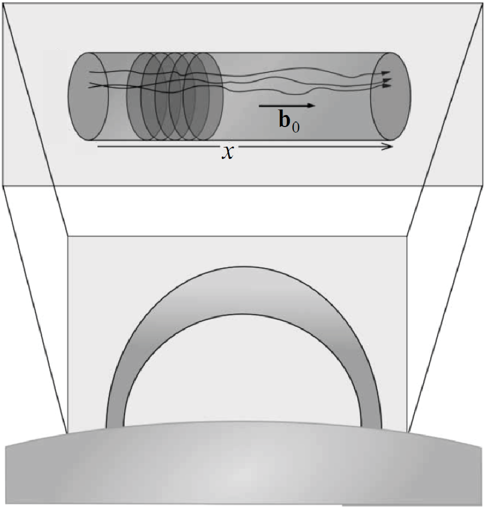

To model a coronal loop, such as the one represented in the left-panel of Fig. 33, kinetic energy is injected at one foot of the coronal loop, with no motion in the other foot . At the motion is non-zero only in the first three shells () and has a Gaussian time distribution. With appropriate values for the different dimensional parameters (motion at , length and radius of the coronal loop, Alfvén wave velocity), and for , Nigro et al. (2004) estimated the time evolution of the total energy, net incoming energy flux and dissipated power (right panel in Fig. 33). This study strongly supports the idea that coronal nanoflares are due to intermittent events produced by Alfvén wave turbulence. About 60% of the energy entering the system is in fact dissipated. The dissipation compares well with the energy involved in nanoflares and, from Fig. 33, clearly displays intermittency with statistics comparable to those of nanoflare emissions. Introducing a more complex model with several layers in , Verdini et al. (2012b) studied the combined effects of turbulence and energy leakage on the coronal heating.
The same RMHD shell model given by Eqs.(307-308) was also used by Verdini and Grappin (2012) to investigate the transition from weak to strong turbulence, depending whether , or , where is the characteristic time responsible for Alfvén waves propagation, and is the eddy turn-over time (see Sec. 2.2.2). In order to prescribe the ratio , they added a forcing term in Eq. (307) leading to an estimation of and at the forcing scale. Typical perpendicular spectra are shown in the left-panel of Fig. 34 for and . They found that (a) only one slope is obtained for strong turbulence, whereas (b) two slopes and are found for weak turbulence. In the notation introduced in Sec. 4.4.1, the weak regime is of (AK) type, in striking opposition with the (KA) isotropic case.


In the context of solar wind MHD turbulence, Verdini et al. (2009) introduced a modified RMHD shell model in the form
| (309) |
where , and stand for the background solar wind, the fluid density and the radius of the magnetic flux tube respectively. The profile of the latter quantities as a function of was assigned along with . The modulus and correlation time of was prescribed at and only in the three first shells. This corresponds to the injection of high frequency Alfvén waves at the base of the chromosphere. By solving Eq. (309) Verdini et al. (2012a) found a double power law for the magnetic frequency spectrum that is reproduced in the right panel of Fig. 34. At low frequency it compares well with the magnetic spectrum of the sub-Alfvénic solar wind represented in Fig. 3. For higher frequencies Verdini et al. (2012a) argue that the -2 slope that they find in their model is masked in the solar wind by the more energetic perpendicular spectrum which has a slope.
4.5 Hall-effect
In strongly magnetized conducting media, e.g. in weakly ionized accretion disks, white dwarfs and neutron stars, the Hall drift of the magnetic field can operate on a much shorter time-scale than the other transport processes. Though non-dissipative, the Hall current redistributes the magnetic energy from large to small scales and thence enhances the dissipation rate of the magnetic field (Urpin and Shalybkov, 1999). The rate of magnetic field decay is important to understanding the history of such astrophysical objects. The Hall effect is probably most pronounced in young neutron stars, called magnetars because of their strong magnetic field of up to G.
In the absence of motion and ambipolar diffusion, the evolution of the magnetic field due to the Hall effect can be written in its dimensionless form as (Goldreich and Reisenegger, 1992)
| (310) |
where , the characteristic magnetic field strength at the largest scale, the elementary charge, the speed of light, the effective mass of an electron and the electron relaxation time.
The last term of Eq. (310) describes the advection of the magnetic field by the Hall drift and is expected to produce a non-linear cascade from large to small magnetic scales. Using the assumption of strong turbulence, Vainshtein (1973) derived a scaling law for the magnetic energy density spectrum. However, considering weakly interacting waves Goldreich and Reisenegger (1992) found an alternative scaling law. In both cases the spectra are steeper than for Kolmogorov turbulence.
The possibility of a cascade is of course appealing for shell models. In addition, for Eq. (310) gives rise to two quadratic invariants, the energy and the magnetic helicity , which are sufficient for the derivation of a shell model including the Hall effect. The difference with MHD shell models is that the non-linear term is now of the form .
Frick et al. (2003) introduced a Hall shell model in the form
| (311) |
with the two quadratic invariants
| (312) |
In Eq.(311) is an externally applied electromotive force and is real. Indeed the real and imaginary parts of complex variables would not couple, as can be seen from Eq. (310) written in Fourier space. We take in order to impose the conservation of magnetic helicity
| (313) |
Solutions of Eq. (311) for (free-decaying Hall-turbulence) show that the initial magnetic energy concentrated in the large scales triggers the cascade process. This results in a magnetic inertial range of the form , corresponding to the Vainshtein (1973) energy density . However, the energy spectrum steepens rapidly in time, unless stochastic forcing is applied (Frick et al., 2007).
On representing the magnetic field as the sum of poloidal and toroidal components, Eq. (310) takes the form (Urpin and Shalybkov, 1999)
| (314) | |||||
| (315) |
From Eqs. (314-315), we clearly see that the two components and are coupled. However, coupling is not symmetric. An initial poloidal configuration can generate a toroidal component with the term . On the other hand, a poloidal component cannot be generated if the initial magnetic configuration is purely toroidal unless some transient dynamo type instability occurs for . Note that, in the presence of a background magnetic field, such a mechanism is at the heart of the so-called Hall drift instability (Rheinhardt and Geppert, 2002). In the context of neutron stars, this instability leads to non-local energy transfer to small scales and then to enhanced crustal field dissipation.
Frick et al. (2003) derived the following shell model for both poloidal and toroidal components of the magnetic field
| (316) | |||
| (317) |
with magnetic energy and magnetic helicity defined by
| (318) |
As in helical models a remarkable advantage of definition (318) is that, contrary to (312), magnetic helicity and magnetic energy are not shell-by-shell correlated. Another advantage is that it is possible to describe the energy exchange between both poloidal and toroidal components of the magnetic field. In particular, it was shown that a transient poloidal field component can develop from an initial purely toroidal configuration (Frick et al., 2003). With again stochastic forcing incorporated into Eqs.(316-317), Frick et al. (2007) found a stable inertial range characterized by the Vainshtein (1973) energy spectrum slope , and .
With the application to the solar wind in mind, Hori et al. (2005) and Galtier and Buchlin (2007) included the Hall effect in the incompressible MHD Eqs. (1-2)
| (319) | |||||
| (320) |
In the limit , the system of Eqs.(319-320) contains three quadratic invariants, the total energy and magnetic helicity defined in Eqs.(5-6), and a third (new) quantity
| (321) |
called the ion helicity. Note that . In the limit , reduces to magnetic helicity, while , also a conserved quantity, reduces to cross helicity .
In the spirit of the complex GOY shell model, the Hall MHD shell model for , takes the form (Hori et al., 2005; Galtier and Buchlin, 2007)
| (323) | |||||
In the limit the following quantities are conserved
| (324) |
with
| (325) |
Note that in Eq. (323) the term accounting for the Hall drift differs from Eq. (311) because here the variables are complex.
Galtier and Buchlin (2007) and Hori and Miura (2008) found that the large-scale magnetic energy density follows a spectrum that steepens to at scales smaller than if the magnetic energy overtakes the kinetic energy or to in the inverse case. This might explain why the magnetic spectrum of the solar wind steepens at high frequencies ().
5 Summary and outlook
Table 3 summarizes the MHD shell models that have been discussed in the present review. The L2 GOY model given by Eqs. (192-) is without doubt the most often used, in its 2D and 3D forms. It gives excellent results in terms of spectra, intermittency, and energy transfer and flux. However, we saw that such a model can be misleading when dealing with kinetic helicity in 3D HD turbulence. This is also true for its cousins the L2 and N2 models given respectively by Eqs. (237-) and Eqs. (234-236). On the other hand helical models do not suffer from this drawback. So far only the H1 local model given by Eq. (264) has been used for MHD turbulence. The other helical models given by Eq. (268) or Eq. (269) are given here for completeness, but have not been tested yet.
As shown in Appendix, the models depicted in Table 3 represent only a subset of all possible models that satisfy total energy and cross helicity conservation. In addition any combination of models will again satisfy both conservation laws. In Table 3 the models which depend on one free parameter are the result of the combination of two other models. Regarding the non-local parameter in Table 3, it controls the degree of non-locality in non-local models. We saw that this parameter can be estimated with the help of a hierarchical approach or from phenomenological arguments (Sec. 3.3).
In addition to automatically satisfying the conservation of total energy and cross helicity, the general formulation given in Eqs. (145-147) has the advantage of offering a mathematical framework for the definition of energy transfer and flux. This general formulation has also been used to define transfer and flux of kinetic helicity in HD turbulence. No doubt it can also be applied to transfer and flux of cross and magnetic helicities in 3D MHD turbulence.
The dimension of MHD turbulence, 2D or 3D, can be changed imposing either the square of magnetic potential or the magnetic helicity as the third quadratic invariant. Though this is possible to achieve for any models, except L1 for which magnetic helicity cannot be defined, in Table 3 we denote by 2D, 3D or both the corresponding version that has been developed so far.
Finally modern shell models always use complex instead of real variables mainly because it increases the degree of freedom of the system, leading to more realistic dynamics.
The applications presented in Sec. 4 correspond to a large panel of situations requiring high values for the kinetic and magnetic Reynolds numbers: small-scale and multi-scale dynamos, free-decaying MHD turbulence, Alfvén wave turbulence and Hall-effect turbulence. In order to deal with anisotropy hybrid models have been developed by mixing 2D MHD turbulence in a plane perpendicular to the direction of anisotropy with direct integration in the parallel direction. A few attempts have been made to develop subgrid shell models, which are indeed an interesting and promising application of shell models.
Shell model simulations require the same time-stepping as direct numerical simulations. However, there is a significant gain in using shell models, essentially because the number of grid points is much lower than in DNS, and partial derivatives are absent. Shell models are user-friendly tools that guide our intuition in realistic parameter regimes still inaccessible to DNS.
| Model | Equations | Variables | Conservative quantities | Comments | Reference |
|---|---|---|---|---|---|
| L1 | (176-178) | real | One free | Gloaguen et al. (1985) | |
| , | parameter | ||||
| L1 | (180-182) | complex | One free | Biskamp (1994) | |
| , | parameter | ||||
| L2 | (192-) | complex | Brandenburg et al. (1996) | ||
| GOY | , | Basu et al. (1998) | |||
| 3D MHD | Frick and Sokoloff (1998) | ||||
| 2D MHD | |||||
| L2 | (237-) | complex | |||
| Sabra | , | Plunian and Stepanov (2007) | |||
| 3D MHD | |||||
| N2 | (), | real | |||
| Hierar- | (220-221) | , | Frik (1984) | ||
| -chical | 2D MHD | ||||
| N2 | (234-236) | complex | One non-local | ||
| , | parameter | Plunian and Stepanov (2007) | |||
| 3D MHD | |||||
| H1 | (264) | complex | One free | ||
| , | parameter | Mizeva et al. (2009) | |||
| 3D MHD | |||||
| H2 | (268) | complex | |||
| (269) | , | This paper | |||
| 3D MHD |
Acknowledgements
This collaboration benefited from the International Research Group Program supported by Perm region Government. R.S. acknowledges the grant YD-4471.2011.1 from the Council of the President of the Russian Federation and the RFBR grant 11-01-96031-ural. P.F. acknowledges the RFBR grant 11-01-00423. We warmly acknowledge J. Torbet for great improvement of the writing.
Appendix A L1-models
The complex L1-models have the form
| (326) |
involving 28 complex coefficients. The number of complex coefficients reduces to 11 on applying the property (147). Then the general shape of complex L1-models becomes
| (327) | |||||
where the are complex parameters. After our definition of L1-models given in Sec. 3.1.2 shell cannot interact with itself only, implying . A similar general shape for complex L1-models has been introduced in the seminal paper by Gloaguen et al. (1985) but using Elsässer variables . Liouville’s theorem yields additional constraints on the possible choice for the . The model given by Eq. (180) investigated by Biskamp (1994) corresponds with taking for .
Appendix B L2-models
Any complex L2-model has the form
| (328) |
A total of 24 complex coefficients are involved. On applying the property (147) the number of complex coefficients is reduced to 12 and the general shape of complex L2-models becomes
where the are again complex parameters. Liouville’s theorem is automatically satisfied as does not depend on , , nor . The GOY model is obtained by setting all coefficients to zero, except and . The Sabra model is obtained by setting all coefficients to zero, except and .
Appendix C N1-models
The N1-models are obtained from the L1-model (327), including the non-local interactions. Their general shape is
| (330) | |||||
where the and are complex parameters depending on . The non-local version of the model (176) by Gloaguen et al. (1985) becomes
| (331) |
where , and are real parameters, and X and Y are real variables.
Appendix D N2-models
The N2-models are obtained from the L2-model (), including the non-local interactions. Their general shape is
where the are again complex parameters depending on . Liouville’s theorem is again automatically satisfied as does not depend on , , nor . Non-local version of GOY and Sabra models is obtained by setting all coefficients to zero, except and for GOY, and and for Sabra.
Appendix E Numerical aspects
Computational gain using a shell model
The computational gain using a shell model rather than a DNS can be estimated. The cost of a simulation is proportional to MN, where M is the number of time steps and N the number of grid points. First we consider HD turbulence.
In each direction the number of grid points can be estimated as the ratio between the scale at which energy is injected and the scale at which energy is dissipated. Defining the Reynolds number at the forcing scale by , with, from Eqs. (20) and (22), and , we find
| (333) |
For a DNS in 3D this leads to
| (334) |
For an isotropic shell model not only is there just one direction, but the sequence of wave numbers is simply geometric. Replacing and in Eq. (333) gives
| (335) |
Therefore the number of grid points in a shell model is about less than in a 3D DNS. Note also that the number of arithmetic operations per variable is about 10 times smaller for a shell model than for a DNS where finite differences are calculated in three directions.
An estimate of the number of time steps is given by the ratio where and are the turn-over times at the forcing and dissipation scales. Assuming Kolmogorov turbulence , we find . Applying Eq. (333) we find
| (336) |
which is the same for DNS and shell models.
In MHD, for the previous estimates hold. However, for the number of grid points in each direction increases by a factor , leading to
| (337) |
and then to
| (338) |
For an isotropic MHD shell model, replacing by and by in Eq. (337) leads to
| (339) |
So for , the number of grid points in a shell model is about less than in a 3D DNS.
An estimate of the number of time steps is now given by the ratio where is the magnetic dissipation time. By definition the latter is given by . With and again then . From Eq. (336) we find
| (340) |
which again is the same for a DNS and a shell model. Note that the number of time steps is approximately the same in HD and MHD, and does not depend on .
Numerical integration
A system of ODEs can be integrated with standard numerical methods like Runge–Kutta. However, special care must be taken because the shell model system of equations is stiff. Indeed as shown before the characteristic times vary considerably between large and small scales by a factor if , or if .
One could think of using a constant time-step equal to the smallest characteristic time of the problem, corresponding here to the dissipation time. However, because the dissipation rate fluctuates strongly, this can lead to a numerical effect of negative viscosity. This is why it is much better to use an adaptive time step, and in addition keeping the latter at least one order of magnitude smaller than the dissipation time.
Another possibility is to split the time-step into two parts, each part solving different physics. During the first part only the non-linear terms are integrated, leading to a value for (in HD). During the second part the exact solution for the dissipative term is calculated, replacing by . This helps to avoid the negative viscosity effect previously mentioned, but it reduces accuracy to a first order approximation .
Stepanov (2002) found another way to increase the accuracy of the method. To explain the method, we write the ODEs system for a HD shell model in the following form
| (341) |
where , and is the quadratic function describing the interactions between shells and with shell . Introducing
| (342) |
the system (341) becomes
| (343) |
Starting with at we want to calculate at . Setting , we calculate using Eq. (343). Then using Eq. (342) we find . Now when calculating , the product of coefficients and with in Eq. (343) can lead to a significant residual error especially at small scales where are much larger than unity. Therefore the numerical integration of Eq. (343) needs to be elaborated a little. Starting with a 4th order Runge-Kutta method, we calculate the explicit quadratic form for in order to avoid in the numerical integration of Eq. (343). This leads to the following numerical scheme
| (344) | |||||
| (345) |
The factors and with can be precalculated only once. The negative viscosity effect is eliminated and the accuracy is up to a fifth order approximation .
More complex methods can be used to deal with stiffness. The VODE time-stepping scheme (Brown et al., 1998) can be used for shell model simulations. The integration method is a variable-coefficient form of Backward Differentiation Formula methods. It requires computing the Jacobian of ODEs. For a local shell model the Jacobian is a sparse matrix. However, for non-local models the Jacobian is a full matrix and the method loses efficiency.
Statistics
In turbulence, the accuracy of e.g. spectral laws and scaling exponents is directly related to the statistics. High accuracy requires to record data over a sufficiently long time, thus again increasing the cost of simulation. Compared to DNS, another advantage of shell models is the possibility to reach accurate statistics.
This was well demonstrated in the study of helicity cascade by Lessinnes et al. (2011). The challenge was to calculate the helicity spectrum resulting from the sum of two quantities , that is zero at leading order and non-zero at next order. The ratio was as small as . A relative error of has been taken in the VODE time scheme. In addition the time fluctuations of were larger than those of energy by a factor , requiring again more data.
In Fig. 35 the results are illustrated for different amounts of data , where is the number of independent runs, each run being performed during time . For a helical forcing (Fig. 35, left panel) we clearly see that does converge to a well-defined spectrum with increasing , while spectra do not change. In the right panel of Fig. 35, is getting smaller with increasing as expected for a non-helical forcing.
The degree of convergence follows the power law in agreement with the following formula
| (346) |
derived for a Gaussian process , where is the standard deviation due to finite sampling of the mean value of , the standard deviation of and the number of independent values of within the sampling.


References
- Alboussière et al. (2011) Alboussière, T., Cardin, P., Debray, F., Rizza, P. L., Masson, J.-P., Plunian, F., Ribeiro, A., Schmitt, D., 2011. Experimental evidence of alfv[e-acute]n wave propagation in a gallium alloy. Physics of Fluids 23 (9), 096601.
- Alemany et al. (2000) Alemany, A., Marty, P., Plunian, F., Soto, J., Jan. 2000. Experimental investigation of dynamo effect in the secondary pumps of the fast breeder reactor Superphenix. Journal of Fluid Mechanics 403, 263–276.
- Alexakis et al. (2007) Alexakis, A., Bigot, B., Politano, H., Galtier, S., Nov 2007. Anisotropic fluxes and nonlocal interactions in magnetohydrodynamic turbulence. Phys. Rev. E 76, 056313.
- Alexakis et al. (2005) Alexakis, A., Mininni, P. D., Pouquet, A., Oct. 2005. Shell-to-shell energy transfer in magnetohydrodynamics. I. Steady state turbulence. Phys. Rev. E72 (4), 046301.
- Alexakis et al. (2006) Alexakis, A., Mininni, P. D., Pouquet, A., 2006. On the inverse cascade of magnetic helicity. The Astrophysical Journal 640 (1), 335.
- Alfvén (1942) Alfvén, H., Oct. 1942. Existence of Electromagnetic-Hydrodynamic Waves. Nat150, 405–406.
- Antonov and Frick (2000) Antonov, T., Frick, P., Jun. 2000. Cascade and scaling in a class of shell models for MHD-turbulence. Mathematical Modelling of Systems and Processes 8, 4–10.
- Antonov et al. (2001) Antonov, T., Frick, P., Sokoloff, D., 2001. Long-time evolution of free-decay mhd turbulence. Doklady Mathematics 63 (2), 271–273.
- Antonov et al. (2001) Antonov, T., Lozhkin, S., Frick, P., Sokoloff, D., Jun. 2001. A shell model for free decaying MHD-turbulence and the role of the magnetic Prandtl number. Magnetohydrodynamics 37, 87–92.
- Aristov and Frik (1988) Aristov, S. N., Frik, P. G., Mar. 1988. Advective flows in a plane rotating layer of a conducting fluid. Magnetohydrodynamics 24 (1), 10–16.
- Aristov and Frik (1989) Aristov, S. N., Frik, P. G., 1989. Large-scale turbulence in a thin layer of a nonisothermal rotating fluid. Fluid Dynamics 23, 522–528.
- Aristov and Frik (1990a) Aristov, S. N., Frik, P. G., 1990a. Large-scale turbulence in Rayleigh-Bénard convection. Fluid Dynamics 24, 690–695.
- Aristov and Frik (1990b) Aristov, S. N., Frik, P. G., Mar. 1990b. Nonlinear effect in the interaction of convective vortices and a magnetic field in a thin layer of a conducting fluid. Magnetohydrodynamics 26 (1), 71–77.
- Aurell et al. (1994a) Aurell, E., Boffetta, G., Crisanti, A., Frick, P., Paladin, G., Vulpiani, A., Dec. 1994a. Statistical mechanics of shell models for two-dimensional turbulence. Phys. Rev. E50, 4705–4715.
- Aurell et al. (1994b) Aurell, E., Frick, P., Shaidurov, V., Apr. 1994b. Hierarchical tree-model of 2D-turbulence. Physica D Nonlinear Phenomena 72, 95–109.
- Avalos-Zuniga and Plunian (2005) Avalos-Zuniga, R., Plunian, F., 2005. Influence of inner and outer walls electromagnetic properties on the onset of a stationary dynamo. The European Physical Journal B - Condensed Matter and Complex Systems 47, 127–135.
- Avalos-Zuniga et al. (2003) Avalos-Zuniga, R., Plunian, F., Gailitis, A., Dec 2003. Influence of electromagnetic boundary conditions onto the onset of dynamo action in laboratory experiments. Phys. Rev. E 68, 066307.
- Barannikov et al. (1988) Barannikov, V. A., Frik, P. G., Shaidurov, V. G., Mar. 1988. Spectral characteristics of two-dimensional turbulent convection in a vertical slot. Journal of Applied Mechanics and Technical Physics 29, 196–200.
- Basu et al. (1998) Basu, A., Sain, A., Dhar, S. K., Pandit, R., Sep. 1998. Multiscaling in Models of Magnetohydrodynamic Turbulence. Physical Review Letters 81, 2687–2690.
- Batchelor and Townsend (1948) Batchelor, G. K., Townsend, A. A., Nov. 1948. Decay of Turbulence in the Final Period. Royal Society of London Proceedings Series A 194, 527–543.
- Bayliss et al. (2007) Bayliss, R. A., Forest, C. B., Nornberg, M. D., Spence, E. J., Terry, P. W., Feb. 2007. Numerical simulations of current generation and dynamo excitation in a mechanically forced turbulent flow. Phys. Rev. E75 (2), 026303.
- Beck et al. (1996) Beck, R., Brandenburg, A., Moss, D., Shukurov, A., Sokoloff, D., 1996. Galactic Magnetism: Recent Developments and Perspectives. Annual Review of Astronomy and Astrophysics 34, 155–206.
- Bell and Nelkin (1978) Bell, T. L., Nelkin, M., Sep. 1978. Time-dependent scaling relations and a cascade model of turbulence. Journal of Fluid Mechanics 88, 369–391.
- Benzi et al. (1996a) Benzi, R., Biferale, L., Kerr, R. M., Trovatore, E., Apr. 1996a. Helical shell models for three-dimensional turbulence. Physics Review E 53, 3541–3550.
- Benzi et al. (1993a) Benzi, R., Biferale, L., Parisi, G., May 1993a. On intermittency in a cascade model for turbulence. Physica D Nonlinear Phenomena 65, 163–171.
- Benzi et al. (1996b) Benzi, R., Biferale, L., Trovatore, E., Oct. 1996b. Universal Statistics of Nonlinear Energy Transfer in Turbulent Models. Physical Review Letters 77, 3114–3117.
- Benzi et al. (1993b) Benzi, R., Ciliberto, S., Tripiccione, R., Baudet, C., Massaioli, F., Succi, S., Jul. 1993b. Extended self-similarity in turbulent flows. Phys. Rev. E48, 29.
- Benzi and Pinton (2010) Benzi, R., Pinton, J., Jul. 2010. Magnetic Reversals in a Simple Model of Magnetohydrodynamics. Physical Review Letters 105 (2), 024501.
- Biferale (1993) Biferale, L., Feb. 1993. Probability distribution functions in turbulent flows and shell models. Physics of Fluids 5, 428–435.
- Biferale (2003) Biferale, L., 2003. Shell Models of Energy Cascade in Turbulence. Annual Review of Fluid Mechanics 35, 441–468.
- Biferale and Kerr (1995) Biferale, L., Kerr, R. M., Dec. 1995. Role of inviscid invariants in shell models of turbulence. Phys. Rev. E52, 6113–6122.
- Biferale et al. (1995) Biferale, L., Lambert, A., Lima, R., Paladin, G., Jan. 1995. Transition to chaos in a shell model of turbulence. Physica D Nonlinear Phenomena 80, 105–119.
- Biskamp (1994) Biskamp, D., Oct. 1994. Cascade models for magnetohydrodynamic turbulence. Phys. Rev. E50, 2702–2711.
- Biskamp (2003) Biskamp, D., 2003. Magnetohydrodynamic Turbulence. Cambridge University Press.
- Biskamp and Müller (1999) Biskamp, D., Müller, W., Sep. 1999. Decay Laws for Three-Dimensional Magnetohydrodynamic Turbulence. Physical Review Letters 83, 2195–2198.
- Bohr et al. (1998) Bohr, T., Jensen, M. H., Paladin, G., Vulpiani, A., 1998. Dynamical Systems Approach to Turbulence. Cambridge University Press.
- Boldyrev (2006) Boldyrev, S., Mar 2006. Spectrum of magnetohydrodynamic turbulence. Phys. Rev. Lett. 96, 115002.
- Boldyrev and Perez (2009) Boldyrev, S., Perez, J. C., Nov 2009. Spectrum of weak magnetohydrodynamic turbulence. Phys. Rev. Lett. 103, 225001.
- Bolgiano (1959) Bolgiano, Jr., R., 1959. Turbulent Spectra in a Stably Stratified Atmosphere. Journal of Geophysical Research 64, 2226–2229.
- Bourgoin et al. (2002) Bourgoin, M., Marié, L., Pétrélis, F., Gasquet, C., Guigon, A., Luciani, J.-B., Moulin, M., Namer, F., Burguete, J., Chiffaudel, A., Daviaud, F., Fauve, S., Odier, P., Pinton, J.-F., Sep. 2002. Magnetohydrodynamics measurements in the von Kármán sodium experiment. Physics of Fluids 14, 3046–3058.
- Brandenburg (1992) Brandenburg, A., Jul. 1992. Energy spectra in a model for convective turbulence. Physical Review Letters 69, 605–608.
- Brandenburg (2001) Brandenburg, A., Apr. 2001. The Inverse Cascade and Nonlinear Alpha-Effect in Simulations of Isotropic Helical Hydromagnetic Turbulence. Astrophysical Journal550, 824–840.
- Brandenburg (2009) Brandenburg, A., Jun. 2009. Large-scale Dynamos at Low Magnetic Prandtl Numbers. Astrophysical Journal697, 1206–1213.
- Brandenburg et al. (1996) Brandenburg, A., Enqvist, K., Olesen, P., Jul. 1996. Large-scale magnetic fields from hydromagnetic turbulence in the very early universe. Phys. Rev. D54, 1291–1300.
- Brandenburg and Subramanian (2005) Brandenburg, A., Subramanian, K., Oct. 2005. Astrophysical magnetic fields and nonlinear dynamo theory. Phys. Rep.417, 1–209.
- Brown et al. (1998) Brown, P. N., Byrne, G. D., Hindmarsh, A. C., Aug. 1998. VODE, a Variable-Coefficient ODE Solver. SIAM. J. Sci. Stat. Comput. 10, 1038–1051.
- Bruno et al. (2005) Bruno, R., Carbone, V., Bavassano, B., Sorriso-Valvo, L. a., 2005. Observations of magnetohydrodynamic turbulence in the 3d heliosphere. Advances in Space Research 35, 939–950.
- Buchlin (2007) Buchlin, É., Oct. 2007. Intermittent heating of the solar corona by MHD turbulence. Nonlinear Processes in Geophysics 14, 649–654.
- Buchlin et al. (2005) Buchlin, E., Galtier, S., Velli, M., Jun. 2005. Influence of the definition of dissipative events on their statistics. A&A436, 355–362.
- Buchlin and Velli (2007) Buchlin, E., Velli, M., Jun. 2007. Shell Models of RMHD Turbulence and the Heating of Solar Coronal Loops. Astrophysical Journal662, 701–714.
- Buchlin, E. (2011) Buchlin, E., 2011. Intermittent turbulent dynamo at very low and high magnetic prandtl numbers. A&A 534, L9.
- Burlaga (1991) Burlaga, L. F., Apr. 1991. Intermittent turbulence in the solar wind. Journal of Geophysical Research 96, 5847–5851.
- Cambon and Jacquin (1989) Cambon, C., Jacquin, J., 1989. Spectral approach to non-isotropic turbulence subjected to rotation. J. Fluid Mech. 202, 295–317.
- Campanelli (2004) Campanelli, L., Oct. 2004. Scaling laws in magnetohydrodynamic turbulence. Phys. Rev. D70 (8), 083009.
- Carati et al. (2006) Carati, D., Debliquy, O., Knaepen, B., Teaca, B., Verma, M., 2006. Energy transfers in forced mhd turbulence. Journal of Turbulence 7, 1–12.
- Carbone (1994a) Carbone, V., Aug. 1994a. Scale similarity of the velocity structure functions in fully developed magnetohydrodynamic turbulence. Phys. Rev. E50, 671.
- Carbone (1994b) Carbone, V., Sep. 1994b. Time Intermittency in a Shell Model for Fully Developed Hydromagnetic Turbulence. Europhysics Letters 27, 581–586.
- Carbone (1995) Carbone, V., Feb. 1995. Signed Measures in a Shell Model for Hydromagnetic Turbulence. Europhysics Letters 29, 377–382.
- Carbone and Veltri (1989) Carbone, V., Veltri, P., Feb. 1989. Discrete scalar cascade models and magnetohydrdynamic turbulence. Phys. of Fluids A 1, 420–425.
- Carbone and Veltri (1990) Carbone, V., Veltri, P., 1990. A shell model for anisotropic magnetohydrodynamic turbulence. Geophysical and Astrophysical Fluid Dynamics 52, 153–181.
- Cattaneo and Hughes (2001) Cattaneo, F., Hughes, D., 2001. Solar dynamo theory: a new look at the origin of small-scale magnetic fields. Astronomy & Geophysics 42, 3.18–3.22.
- Cattaneo and Hughes (2009) Cattaneo, F., Hughes, D., 2009. Problems with kinematic mean field electrodynamics at high magnetic reynolds numbers. Mon. Not. R. Astron. Soc. 395, L48–L51.
- Cattaneo and Tobias (2009) Cattaneo, F., Tobias, S. M., Feb. 2009. Dynamo properties of the turbulent velocity field of a saturated dynamo. Journal of Fluid Mechanics 621, 205.
- Chakraborty et al. (2010) Chakraborty, S., Jensen, M. H., Sarkar, A., Feb. 2010. On two-dimensionalization of three-dimensional turbulence in shell models. European Physical Journal B 73, 447–453.
- Chen et al. (2003) Chen, Q., Chen, S., Eyink, G. L., 2003. The joint cascade of energy and helicity in three-dimensional turbulence. Physics of Fluids 15 (2), 361–374.
- Childress and Gilbert (1995) Childress, S., Gilbert, A., 1995. Stretch, Twist, Fold: the fast dynamo. Springer.
- Christensson et al. (2005) Christensson, M., Hindmarsh, M., Brandenburg, A., 2005. Scaling laws in decaying helical hydromagnetic turbulence. Astronomische Nachrichten 326 (6), 393–399.
- Courvoisier et al. (2010) Courvoisier, A., Hughes, D., Proctor, M., 2010. A self-consistent treatment of the electromotive force in magnetohydrodynamics for large diffusivities. Astronomische Nachrichten 331 (7), 667–670.
- Craya (1958) Craya, A., 1958. Contribution à l’analyse de la turbulence associée à des vitesses moyennes. P.S.T. Ministère de l’Air (Paris) 345.
- Davidson (2001) Davidson, P. A., 2001. An Introduction to Magnetohydrodynamics. Cambridge University Press.
- Desnianskii and Novikov (1974) Desnianskii, V. N., Novikov, E. A., 1974. Simulation of cascade processes in turbulent flows. Prikladnaia Matematika i Mekhanika 38, 507–513.
- Ditlevsen (2011) Ditlevsen, P., 2011. Turbulence and Shell Models. Cambridge University Press.
- Ditlevsen and Giuliani (2001a) Ditlevsen, P. D., Giuliani, P., Mar. 2001a. Cascades in helical turbulence. Physics Review E 63 (3), 036304.
- Ditlevsen and Giuliani (2001b) Ditlevsen, P. D., Giuliani, P., 2001b. Dissipation in helical turbulence. Physics of Fluids 13 (11), 3508–3509.
- Dobler et al. (2003) Dobler, W., Frick, P., Stepanov, R., May 2003. Screw dynamo in a time-dependent pipe flow. Phys. Rev. E67 (5), 056309.
- Dombre and Gilson (1998) Dombre, T., Gilson, J., Jan. 1998. Intermittency, chaos and singular fluctuations in the mixed Obukhov-Novikov shell model of turbulence. Physica D Nonlinear Phenomena 111, 265–287.
- Fournier et al. (1982) Fournier, J.-D., Sulem, P.-L., Pouquet, A., Apr. 1982. Infrared properties of forced magnetohydrodynamic turbulence. Journal of Physics A Mathematical General 15, 1393–1420.
- Frick (2003) Frick, P., 2003. Turbulence approaches and models. Regular and chaotic dynamics, Moscow-Ijevsk.
- Frick et al. (2000) Frick, P., Boffetta, G., Giuliani, P., Lozhkin, S., Sokoloff, D., Dec. 2000. Long-time behavior of MHD shell models. Europhysics Letters 52, 539–544.
- Frick et al. (1995) Frick, P., Dubrulle, B., Babiano, A., Jun. 1995. Scaling properties of a class of shell models. Phys. Rev. E51, 5582–5593.
- Frick et al. (2002) Frick, P., Noskov, V., Denisov, S., Khripchenko, S., Sokoloff, D., Stepanov, R., Sukhanovsky, A., 2002. Non-stanionary screw flow in a toroidal channel: way to a laboratory dynamo experiment. Magnetohydrodynamics 38 (1-2), 143–162.
- Frick et al. (2010) Frick, P., Noskov, V., Denisov, S., Stepanov, R., Oct 2010. Direct measurement of effective magnetic diffusivity in turbulent flow of liquid sodium. Phys. Rev. Lett. 105 (18), 184502.
- Frick et al. (2002) Frick, P., Reshetnyak, M., Sokoloff, D., Jul. 2002. Combined grid-shell approach for convection in a rotating spherical layer. Europhysics Letters 59, 212–217.
- Frick and Sokoloff (1998) Frick, P., Sokoloff, D., Apr. 1998. Cascade and dynamo action in a shell model of magnetohydrodynamic turbulence. Phys. Rev. E57, 4155–4164.
- Frick and Stepanov (2010) Frick, P., Stepanov, R., Nov. 2010. Long-term free decay of MHD turbulence. Europhysics Letters 92, 34007.
- Frick et al. (2003) Frick, P., Stepanov, R., Nekrasov, V., Sep. 2003. Shell model of magnetic field evolution under the Hall effect. Magnetohydrodynamics 39, 327–334.
- Frick et al. (2007) Frick, P., Stepanov, R., Rheinhardt, M., Aug. 2007. Shell models for Hall effect induced magnetic turbulence. New Journal of Physics 9, 293.
- Frick et al. (2006) Frick, P., Stepanov, R., Sokoloff, D., Dec. 2006. Large- and small-scale interactions and quenching in an -dynamo. Phys. Rev. E74 (6), 066310.
- Frick and Zimin (1993) Frick, P. G., Zimin, V. D., 1993. Hierarchical models of turbulence. In: Farge, M., Hunt, J. C. R., Vassilicos, J. C. (Eds.), Wavelets, fractals and Fourier transform: new developments and new applications. Cambridge, Oxford Press, p. 256.
- Frik (1983) Frik, P. G., Mar. 1983. Hierarchical model of two-dimensional turbulence. Magnetohydrodynamics 19 (1), 48–53.
- Frik (1984) Frik, P. G., Sep. 1984. Two-dimensional MHD turbulence - A hierarchical model. Magnetohydrodynamics 20 (3), 262–267.
- Frik (1986) Frik, P. G., Mar. 1986. Modeling cascade processes in two-dimensional turbulent convection. Journal of Applied Mechanics and Technical Physics 27, 221–228.
- Frik (1987) Frik, P. G., 1987. Modeling of the space-time structure of developed two-dimensional turbulent convection. Fluid Mechanics - Soviet Research 16 (3), 49–54.
- Frisch (1995) Frisch, U., 1995. Turbulence. Cambridge University Press.
- Frisch et al. (1975) Frisch, U., Pouquet, A., L�orat, J., Mazure, A., 1975. Possibility of an inverse cascade of magnetic helicity in magnetohydrodynamic turbulence. J. Fluid Mech. 68, 769–778.
- Frisch et al. (1987) Frisch, U., She, Z. S., Sulem, P. L., Oct. 1987. Large-scale flow driven by the anisotropic kinetic alpha effect. Physica D Nonlinear Phenomena 28, 382–392.
- Gailitis et al. (2000) Gailitis, A., Lielausis, O., Dement’ev, S., Platacis, E., Cifersons, A., Gerbeth, G., Gundrum, T., Stefani, F., Christen, M., Hänel, H., Will, G., May 2000. Detection of a flow induced magnetic field eigenmode in the riga dynamo facility. Phys. Rev. Lett. 84, 4365–4368.
- Galtier and Buchlin (2007) Galtier, S., Buchlin, E., Feb. 2007. Multiscale Hall-Magnetohydrodynamic Turbulence in the Solar Wind. Astrophysical Journal656, 560–566.
- Galtier et al. (2000) Galtier, S., Nazarenko, S. V., Newell, A. C., Pouquet, A., 2000. A weak turbulence theory for incompressible magnetohydrodynamics. Journal of Plasma Physics 63 (05), 447–488.
- Geertsema and Achterberg (1992) Geertsema, G. T., Achterberg, A., Feb. 1992. Turbulence in differentially rotating thin disks - A multi-component cascade model. A&A255, 427–442.
- Gekelman (1999) Gekelman, W., 1999. Review of laboratory experiments on alfv�n waves and their relationship to space observations. Journal of Geophysical Research 104, 14417–14435.
- Giuliani and Carbone (1998) Giuliani, P., Carbone, V., Sep. 1998. A note on shell models for MHD turbulence. Europhysics Letters 43, 527–532.
- Gledzer (1973) Gledzer, E. B., Oct. 1973. System of hydrodynamic type admitting two quadratic integrals of motion. Soviet Physics Doklady 18, 216.
- Gledzer et al. (1981) Gledzer, E. B., Dolzhanskii, F. B., Obukhov, A. M., 1981. Systems of hydrodynamic type and their applications. Nauka, in Russian.
- Gledzer and Makarov (1979) Gledzer, E. B., Makarov, A. L., Sep. 1979. Construction of a cascade model of two-dimensional turbulence. Akademiia Nauk SSSR Fizika Atmosfery i Okeana 15, 899–906.
- Gloaguen et al. (1985) Gloaguen, C., Léorat, J., Pouquet, A., Grappin, R., 1985. A scalar model for mhd turbulence. Physica D: Nonlinear Phenomena 17 (2), 154 – 182.
- Glukhovskii (1975) Glukhovskii, A. B., Dec. 1975. The effect of the value of the scale splitting coefficient on the stability of chain-type nonlinear systems. Akademiia Nauk SSSR Fizika Atmosfery i Okeana 11, 1323–1326.
- Goldreich and Reisenegger (1992) Goldreich, P., Reisenegger, A., Aug. 1992. Magnetic field decay in isolated neutron stars. Astrophysical Journal395, 250–258.
- Goldreich and Sridhar (1995) Goldreich, P., Sridhar, S., Jan. 1995. Toward a theory of interstellar turbulence. 2: Strong alfvenic turbulence. Astrophysical Journal438, 763–775.
- Golitsyn (1960) Golitsyn, G. S., 1960. Magnetic field and current density fluctuations in a turbulent flow of weak conductive fluid. Dokl. Akad. Nauk. SSSR 132, 315–318.
- Gotoh et al. (2002) Gotoh, T., Fukayama, D., Nakano, T., 2002. Velocity field statistics in homogeneous steady turbulence obtained using a high-resolution direct numerical simulation. Physics of Fluids 14 (3), 1065–1081.
- Grappin et al. (1986) Grappin, R., Léorat, J., Pouquet, A., 1986. Computation of the dimension of a model of fully developed turbulence. Journal de Physique 47, 1127 – 1136.
- Grauer et al. (1994) Grauer, R., Krug, J., Marliani, C., Dec. 1994. Scaling of high-order structure functions in magnetohydrodynamic turbulence. Physics Letters A 195, 335–338.
- Hattori et al. (2001) Hattori, Y., , Ishizawa, A., 2001. Characteristic Time Scales and Energy Transfer in MHD Turbulence. Proceedings of IUTAM Symposium on Geometry and Statistics of Turbulence, 89–94.
- Hattori et al. (2004) Hattori, Y., Rubinstein, R., Ishizawa, A., Oct. 2004. Shell model for rotating turbulence. Phys. Rev. E70 (4), 046311.
- Herring (1974) Herring, J. R., 1974. Approach of axisymmetric turbulence to isotropy. Phys. Fluids 17, 859–872.
- Horbury and Balogh (1997) Horbury, T. S., Balogh, A., 1997. Structure function measurements of the intermittent mhd turbulent cascade. Nonlinear Processes in Geophysics 4, 185–199.
- Horbury et al. (2008) Horbury, T. S., Forman, M., Oughton, S., Oct 2008. Anisotropic scaling of magnetohydrodynamic turbulence. Phys. Rev. Lett. 101, 175005.
- Hori et al. (2005) Hori, D., Furukawa, M., Ohsaki, S., Yoshida, Z., 2005. A Shell Model for the Hall MHD System. Journal of Plasma and Fusion Research 81, 141–142.
- Hori and Miura (2008) Hori, D., Miura, H., 2008. Spectrum Properties of Hall MHD Turbulence. Plasma and Fusion Research 3, 1053.
- Howes et al. (2011) Howes, G. G., TenBarge, J. M., Dorland, W., 2011. A weakened cascade model for turbulence in astrophysical plasmas. Physics of Plasmas 18 (10), 102305.
- Iroshnikov (1964) Iroshnikov, P. S., Feb. 1964. Turbulence of a Conducting Fluid in a Strong Magnetic Field. Soviet Astronomy 7, 566–571, trans. from Astron. Zh., 40, 4, 742-750 (1963).
- Iskakov et al. (2007) Iskakov, A. B., Schekochihin, A. A., Cowley, S. C., McWilliams, J. C., Proctor, M. R. E., May 2007. Numerical demonstration of fluctuation dynamo at low magnetic prandtl numbers. Phys. Rev. Lett. 98, 208501.
- Jensen (1991) Jensen, M. H., 1991. Models of turbulence. Physica Scripta T38, 22–27.
- Kadanoff et al. (1995) Kadanoff, L., Lohse, D., Wang, J., Benzi, R., 1995. Scaling and dissipation in the goy shell model. Phys. Fluids 7, 617–629.
- Kerr and Siggia (1978) Kerr, R. M., Siggia, E. D., Nov. 1978. Cascade model of fully developed turbulence. Journal of Statistical Physics 19, 543–552.
- Kolmogorov (1941) Kolmogorov, A., 1941. The local structure of turbulence in incompressible viscous fluid for very large reynolds numbers. Dokl. Akad. Nauk. SSSR 30, 299–303.
- Kraichnan (1965) Kraichnan, R. H., Jul. 1965. Inertial-Range Spectrum of Hydromagnetic Turbulence. Physics of Fluids 8, 1385–1387.
- Kraichnan (1973) Kraichnan, R. H., 1973. Helical turbulence and absolute equilibrium. Journal of Fluid Mechanics 59, 745–752.
- Krause and Rädler (1980) Krause, F., Rädler, K.-H., 1980. Mean-field magnetos and dynamo theory. Akademie-Verlag Berlin.
- Lesieur (1997) Lesieur, M., 1997. Turbulence in Fluids (3rd revised and enlarged edition). Kluwer Academic.
- Lessinnes (2010) Lessinnes, T., 2010. Modélisation de la turbulence magnétohydrodynamique. Application à l’effet dynamo. Ph.D. thesis, Université Libre de Bruxelles.
- Lessinnes et al. (2009a) Lessinnes, T., Carati, D., Verma, M. K., Jun. 2009a. Energy transfers in shell models for magnetohydrodynamics turbulence. Phys. Rev. E79 (6), 066307.
- Lessinnes et al. (2009b) Lessinnes, T., Plunian, F., Carati, D., Nov. 2009b. Helical shell models for MHD. Theoretical and Computational Fluid Dynamics 23, 439–450.
- Lessinnes et al. (2011) Lessinnes, T., Plunian, F., Stepanov, R., Carati, D., 2011. Dissipation scales of kinetic helicities in turbulence. Physics of Fluids 23 (3), 035108.
- Lorenz (1971) Lorenz, E. N., 1971. Investigating the predictability of turbulent motion. Lecture Notes in Physics 12, 195–204.
- Lorenz (1972) Lorenz, E. N., 1972. Low order models representing realizations of turbulence. Journal of Fluid Mechanics 55, 545–563.
- L’vov et al. (1998) L’vov, V. S., Podivilov, E., Pomyalov, A., Procaccia, I., Vandembroucq, D., Aug. 1998. Improved shell model of turbulence. Phys. Rev. E58, 1811–1822.
- Mason et al. (2008) Mason, J., Cattaneo, F., Boldyrev, S., Mar 2008. Numerical measurements of the spectrum in magnetohydrodynamic turbulence. Phys. Rev. E 77, 036403.
- Melander (1997) Melander, M. V., Feb. 1997. Helicity Causes Chaos in a Shell Model of Turbulence. Physical Review Letters 78, 1456–1459.
- Melander and Fabijonas (2002) Melander, M. V., Fabijonas, B. R., Jul. 2002. Self-similar enstrophy divergence in a shell model of isotropic turbulence. Journal of Fluid Mechanics 463, 241–258.
- Melander and Fabijonas (2003) Melander, M. V., Fabijonas, B. R., Apr. 2003. Transients in the decay of isotropic turbulence. Journal of Turbulence 4, 14.
- Melander and Fabijonas (2006) Melander, M. V., Fabijonas, B. R., 2006. A theory of inertial range similarity in isotropic turbulence. Physica D 75275, 4.
- Merrill and McElhinny (1983) Merrill, R. T., McElhinny, W. M., 1983. The Earth’s Magnetic Field: Its History, Origin and Planetary Perspective. Elsevier New York.
- Mininni et al. (2005) Mininni, P., Alexakis, A., Pouquet, A., Oct. 2005. Shell-to-shell energy transfer in magnetohydrodynamics. II. Kinematic dynamo. Phys. Rev. E72 (4), 046302.
- Mizeva et al. (2009) Mizeva, I. A., Stepanov, R. A., Frik, P. G., Feb. 2009. The cross-helicity effect on cascade processes in MHD turbulence. Physics - Doklady 54, 93–97.
- Moffatt (1978) Moffatt, H., 1978. Magnetic field generation in electrically conducting fluids. Cambridge University Press.
- Moffatt (1961) Moffatt, K., 1961. The amplification of a weak applied magnetic field by turbulence in fluids of moderate conductivity. Journal of Fluid Mechanics 11 (04), 625–635.
- Monchaux et al. (2007) Monchaux, R., Berhanu, M., Bourgoin, M., Moulin, M., Odier, P., Pinton, J.-F., Volk, R., Fauve, S., Mordant, N., Pétrélis, F., Chiffaudel, A., Daviaud, F., Dubrulle, B., Gasquet, C., Marié, L., Ravelet, F., Jan 2007. Generation of a magnetic field by dynamo action in a turbulent flow of liquid sodium. Phys. Rev. Lett. 98 (4), 044502.
- Moreau (1990) Moreau, R., 1990. Magnetohydrodynamics. Kluwer Academic.
- Morin and Dormy (2009) Morin, V., Dormy, E., Nov. 2009. The dynamo bifurcation in rotating spherical shells . International Journal of Modern Physics B 23, 5467–5482.
- Müller and Biskamp (2000) Müller, W.-C., Biskamp, D., Jan. 2000. Scaling Properties of Three-Dimensional Magnetohydrodynamic Turbulence. Physical Review Letters 84, 475–478.
- Müller et al. (2003) Müller, W.-C., Biskamp, D., Grappin, R., Jun 2003. Statistical anisotropy of magnetohydrodynamic turbulence. Phys. Rev. E 67 (6), 066302.
- Müller and Grappin (2005) Müller, W.-C., Grappin, R., Sep. 2005. Spectral Energy Dynamics in Magnetohydrodynamic Turbulence. Physical Review Letters 95 (11), 114502.
- Nataf et al. (2008) Nataf, H.-C., Alboussi‘ere, T., Brito, D., Cardin, P., Gagni�re, N., Jault, D., Schmitt, D., 2008. Rapidly rotating spherical couette flow in a dipolar magnetic field: An experimental study of the mean axisymmetric flow. Physics of the Earth and Planetary Interiors 170 (1-2), 60 – 72.
- Nigro and Carbone (2010) Nigro, G., Carbone, V., Jul. 2010. Magnetic reversals in a modified shell model for magnetohydrodynamics turbulence. Phys. Rev. E82 (1), 016313.
- Nigro et al. (2004) Nigro, G., Malara, F., Carbone, V., Veltri, P., May 2004. Nanoflares and MHD Turbulence in Coronal Loops: A Hybrid Shell Model. Physical Review Letters 92 (19), 194501.
- Nigro et al. (2005) Nigro, G., Malara, F., Veltri, P., Aug. 2005. Large-Amplitude Velocity Fluctuations in Coronal Loops: Flare Drivers? Astrophysical Journal Letters629, L133–L136.
- Nigro and Veltri (2011) Nigro, G., Veltri, P., 2011. A study of the dynamo transition in a self-consistent nonlinear dynamo model. The Astrophysical Journal Letters 740 (2), L37.
- Obukhov (1941) Obukhov, A., 1941. On the energy distribution in a turbulent flow spectrum. Izvestiya Akademii Nauk SSSR, Seria Geofizika 4-5, 453–466.
- Obukhov (1959) Obukhov, A., 1959. On the influence of archimedean force on structure of the turbulent field in a turbulent flow. Dokl. Akad. Nauk SSSR 125, 1246–1248.
- Obukhov (1971) Obukhov, A., 1971. On some general characteristic equations of the dynamics of the atmosphere. Izvestiya Akademii Nauk SSSR, Fizika Atmosfery i Okeana 7, 695–704.
- Odier et al. (1998) Odier, P., Pinton, J.-F., Fauve, S., Dec 1998. Advection of a magnetic field by a turbulent swirling flow. Phys. Rev. E 58, 7397–7401.
- Ott et al. (1992) Ott, E., Du, Y., Sreenivasan, K. R., Juneja, A., Suri, A. K., Nov. 1992. Sign-singular measures - Fast magnetic dynamos, and high-Reynolds-number fluid turbulence. Physical Review Letters 69, 2654–2657.
- Pétrélis and Fauve (2001) Pétrélis, F., Fauve, S., Aug. 2001. Saturation of the magnetic field above the dynamo threshold. European Physical Journal B 22, 273–276.
- Pétrélis and Fauve (2008) Pétrélis, F., Fauve, S., Dec. 2008. Chaotic dynamics of the magnetic field generated by dynamo action in a turbulent flow. Journal of Physics Condensed Matter 20, 4203.
- Pétrélis et al. (2009) Pétrélis, F., Fauve, S., Dormy, E., Valet, J.-P., Apr. 2009. Simple Mechanism for Reversals of Earth’s Magnetic Field. Physical Review Letters 102 (14), 144503.
- Peyrot et al. (2008) Peyrot, M., Gilbert, A., Plunian, F., 2008. Oscillating ponomarenko dynamo in the highly conducting limit. Physics of Plasmas 15 (12), 122104.
- Peyrot et al. (2007) Peyrot, M., Plunian, F., Normand, C., 2007. Parametric instability of the helical dynamo. Physics of Fluids 19 (5), 054109.
- Pisarenko et al. (1993) Pisarenko, D., Biferale, L., Courvoisier, D., Frisch, U., Vergassola, M., Oct. 1993. Further results on multifractality in shell models. Physics of Fluids 5, 2533–2538.
- Plunian et al. (1999) Plunian, F., Marty, P., Alemany, A., 1999. Kinematic dynamo action in a network of screw motions; application to the core of a fast breeder reactor. Journal of Fluid Mechanics 382, 137–154.
- Plunian and Stepanov (2007) Plunian, F., Stepanov, R., Aug. 2007. A non-local shell model of hydrodynamic and magnetohydrodynamic turbulence. New Journal of Physics 9, 294.
- Plunian and Stepanov (2010) Plunian, F., Stepanov, R., Oct. 2010. Cascades and dissipation ratio in rotating magnetohydrodynamic turbulence at low magnetic Prandtl number. Phys. Rev. E82 (4), 046311.
- Politano and Pouquet (1995) Politano, H., Pouquet, A., Jul. 1995. Model of intermittency in magnetohydrodynamic turbulence. Phys. Rev. E52, 636–641.
- Ponty et al. (2005) Ponty, Y., Mininni, P. D., Montgomery, D. C., Pinton, J.-F., Politano, H., Pouquet, A., Apr. 2005. Numerical Study of Dynamo Action at Low Magnetic Prandtl Numbers. Physical Review Letters 94 (16), 164502.
- Ponty and Plunian (2011) Ponty, Y., Plunian, F., Apr 2011. Transition from large-scale to small-scale dynamo. Phys. Rev. Lett. 106, 154502.
- Pope (2000) Pope, S. B., 2000. Turbulent flows. Cambridge.
- Pouquet et al. (1976) Pouquet, A., Frisch, U., Leorat, J., Sep. 1976. Strong MHD helical turbulence and the nonlinear dynamo effect. Journal of Fluid Mechanics 77, 321–354.
- Rädler (2007a) Rädler, K.-H., 2007a. Mean-field dynamo theory: early ideas and today’s problems. In: S. Molokov, R. M., Moffatt, H. K. (Eds.), Magnetohydrodynamics: Historical Evolution and Trends. Springer, pp. 55–72.
- Rädler (2007b) Rädler, K.-H., 2007b. Mean-field dynamos. In: Gubbins, D., Herrero-Bervera, E. (Eds.), Encyclopedia of Geomagnetism and Paleomagnetism. Springer, pp. 192–199.
- Ravelet et al. (2008) Ravelet, F., Berhanu, M., Monchaux, R., Aumaître, S., Chiffaudel, A., Daviaud, F., Dubrulle, B., Bourgoin, M., Odier, P., Plihon, N., Pinton, J.-F., Volk, R., Fauve, S., Mordant, N., Pétrélis, F., Aug 2008. Chaotic dynamos generated by a turbulent flow of liquid sodium. Phys. Rev. Lett. 101, 074502.
- Rheinhardt and Geppert (2002) Rheinhardt, M., Geppert, U., Mar. 2002. Hall-Drift Induced Magnetic Field Instability in Neutron Stars. Phys. Rev. Lett. 88, 101103+.
- Rowlands et al. (2005) Rowlands, G., Chapman, S. C., Hnat, B., Dec. 2005. Extended Self Similarity in Solar Wind Turbulence. AGU Fall Meeting Abstracts.
- Ruzmaikin et al. (1988) Ruzmaikin, A. A., Sokoloff, D. D., Shukurov, A. M., 1988. Magnetic Fields of Galaxies. Kluwer, Dordrecht.
- Ryan and Sarson (2007) Ryan, D. A., Sarson, G. R., Jan. 2007. Are geomagnetic field reversals controlled by turbulence within the Earth’s core? Geophysical Research Letters34, L02307.
- Ryan and Sarson (2011) Ryan, D. A., Sarson, G. R., Oct. 2011. A coupled low order dynamo/turbulent shell model for geomagnetic field variations and reversals. Physics of the Earth and Planetary Interiors 188, 214–234.
- Saddoughi and Veeravalli (1994) Saddoughi, S., Veeravalli, S., 1994. Local isotropy in turbulent layers at high reynolds number. J. Fluid Mech. 268, 333–372.
- Saffman (1967) Saffman, P., G., 1967. Note on decay of homogeneous turbulence. Phys 10, 1349.
- Sakuraba and Roberts (2009) Sakuraba, Roberts, 2009. Generation of a strong magnetic field using uniform heat flux at the surface of the core. Nature Geoscience 2, 802–805.
- Schaeffer et al. (2011) Schaeffer, N., Jault, D., Cardin, P., Drouard, M., Dec. 2011. On the reflection of Alfvén waves and its implication for Earth’s core modeling. ArXiv e-prints 1112.3879.
- Schekochihin and Cowley (2007) Schekochihin, A. A., Cowley, S. C., 2007. Turbulence and Magnetic Fields in Astrophysical Plasmas. In: Molokov, S., Moreau, R., & Moffatt, H. K. (Ed.), Magnetohydrodynamics: Historical Evolution and Trends. Springer, p. 85.
- Schekochihin et al. (2002) Schekochihin, A. A., Cowley, S. C., Hammett, G. W., Maron, J. L., McWilliams, J. C., Oct. 2002. A model of nonlinear evolution and saturation of the turbulent MHD dynamo. New Journal of Physics 4, 84.
- Schekochihin et al. (2004) Schekochihin, A. A., Cowley, S. C., Maron, J. L., McWilliams, J. C., Feb. 2004. Critical Magnetic Prandtl Number for Small-Scale Dynamo. Physical Review Letters 92 (5), 054502.
- Schekochihin et al. (2004) Schekochihin, A. A., Cowley, S. C., Taylor, S. F., Maron, J. L., McWilliams, J. C., 2004. Simulations of the small-scale turbulent dynamo. The Astrophysical Journal 612 (1), 276.
- Shaidurova (1987) Shaidurova, T., 1987. Hierarchical models of turbulence (in russian). Ph.D. thesis, Perm State University.
- Shakura and Sunyaev (1973) Shakura, N. I., Sunyaev, R. A., 1973. Black holes in binary systems. Observational appearance. A&A24, 337–355.
- She and Leveque (1994) She, Z.-S., Leveque, E., Jan. 1994. Universal scaling laws in fully developed turbulence. Physical Review Letters 72, 336–339.
- Shew and Lathrop (2005) Shew, W. L., Lathrop, D. P., 2005. Liquid sodium model of geophysical core convection. Physics of the Earth and Planetary Interiors 153 (1�3), 136 – 149.
- Sokoloff and Frick (2003) Sokoloff, D. D., Frick, P. G., Jun. 2003. Model of a Multiscaled MHD Dynamo. Astronomy Reports 47, 511–516.
- Spence et al. (2007) Spence, E. J., Nornberg, M. D., Jacobson, C. M., Parada, C. A., Taylor, N. Z., Kendrick, R. D., Forest, C. B., Apr 2007. Turbulent diamagnetism in flowing liquid sodium. Phys. Rev. Lett. 98, 164503.
- Steenbeck et al. (1966) Steenbeck, M., Krause, F., Rädler, K.-H., 1966. Berechnung der mittleren Lorentz-Feldstärke für ein elektrisch leitendes Medium in turbulenter, durch Coriolis-Kräfte beeinfluster Bewegung. Z. Naturforsch. 21a, 369–376.
- Stepanov (2002) Stepanov, R., 2002. Optimization of numerical integration methods for shell models. Numerical Methods and Programming 3, 176–179.
- Stepanov et al. (2006) Stepanov, R., Frick, P., Sokoloff, D., Jun. 2006. A multi-scale disk dynamo model. Astronomische Nachrichten 327, 481.
- Stepanov et al. (2008) Stepanov, R., Frick, P., Sokoloff, D., Jun. 2008. Coupling of mean-field equation and shell model of turbulence in the context of galactic dynamo probleml. Computation continous mechanics 1, 97–108.
- Stepanov and Plunian (2006) Stepanov, R., Plunian, F., 2006. Fully developed turbulent dynamo at low magnetic Prandtl numbers. Journal of Turbulence 7, 39.
- Stepanov and Plunian (2008) Stepanov, R., Plunian, F., Jun. 2008. Phenomenology of Turbulent Dynamo Growth and Saturation. Astrophysical Journal680, 809–815.
- Stepanov et al. (2009) Stepanov, R. A., Frik, P. G., Shestakov, A. V., Nov. 2009. Spectral properties of helical turbulence. Fluid Dynamics 44, 658–666.
- Stieglitz and Müller (2001) Stieglitz, R., Müller, U., 2001. Experimental demonstration of a homogeneous two-scale dynamo. Physics of Fluids 13 (3), 561–564.
- Strauss (1976) Strauss, H. R., 1976. Nonlinear, three-dimensional magnetohydrodynamics of noncircular tokamaks. Physics of Fluids 19 (1), 134–140.
- Teaca et al. (2009) Teaca, B., Verma, M. K., Carati, D., 2009. Energy transfers in magnetohydrodynamic turbulence in presence of an ambiant imposed magnetic field. Physics AUC 19, 22–34.
- Teaca et al. (2009) Teaca, B., Verma, M. K., Knaepen, B., Carati, D., APR 2009. Energy transfer in anisotropic magnetohydrodynamic turbulence. Phys. Rev. E79 (4).
- Tobias et al. (2011) Tobias, S. M., Cattaneo, F., Boldyrev, S., 2011. Mhd dynamos and turbulence. In: Davidson, P., Kaneda, Y., Sreenivassan, K. R. (Eds.), Ten Chapters in Turbulence. Cambridge University Press, pp. 351–404.
- Uritsky et al. (2010) Uritsky, V. M., Pouquet, A., Rosenberg, D., Mininni, P. D., Donovan, E. F., Nov. 2010. Structures in magnetohydrodynamic turbulence: Detection and scaling. Phys. Rev. E82 (5), 056326.
- Urpin and Shalybkov (1999) Urpin, V., Shalybkov, D., Apr. 1999. Magnetohydrodynamic processes in strongly magnetized young neutron stars. MNRAS304, 451–456.
- Vainshtein (1973) Vainshtein, S., 1973. Strong plasma turbulence at helicon frequencies. Soviet Physics JETP 37, 73.
- Verdini and Grappin (2012) Verdini, A., Grappin, R., 2012. Transition from weak to strong cascade in mhd turbulence. Phys. Rev. Lett. 109, 025004.
- Verdini et al. (2012a) Verdini, A., Grappin, R., Pinto, R., Velli, M., 2012a. On the origin of the 1/f spectrum in the solar wind magnetic field. The Astrophysical Journal Letters 750 (2), L33.
- Verdini et al. (2012b) Verdini, A., Grappin, R., Velli, M., 2012b. Coronal heating in coupled photosphere-chromosphere-coronal systems: turbulence and leakage. A&A538, 70.
- Verdini et al. (2009) Verdini, A., Velli, M., Buchlin, E., Jul. 2009. Turbulence in the Sub-Alfvénic Solar Wind Driven by Reflection of Low-Frequency Alfvén Waves. Astrophysical Journal Letters700, L39–L42.
- Verma (2004) Verma, M. K., Nov. 2004. Statistical theory of magnetohydrodynamic turbulence: recent results. Phys. Rep.401, 229–380.
- Vishniac et al. (2003) Vishniac, E., Lazarian, A., Cho, J., 2003. Problems and progresses in astrophysical dynamo. In: Falgarone, E., Passot, T. (Eds.), Turbulence and magnetic fields in astrophysics. Springer, pp. 376–401.
- Waleffe (1992) Waleffe, F., 1992. The nature of triad interactions in homogeneous turbulence. Physics of Fluids A: Fluid Dynamics 4 (2), 350–363.
- Weiss and Thompson (2009) Weiss, N., Thompson, M., 2009. The Solar Dynamo. Space Sci Rev 144, 53–66.
- Yakhot and Zakharov (1993) Yakhot, V., Zakharov, V., Apr. 1993. Hidden conservation laws in hydrodynamics; energy and dissipation rate fluctuation spectra in strong turbulence. Physica D Nonlinear Phenomena 64, 379–394.
- Yamada and Ohkitani (1987) Yamada, M., Ohkitani, K., Dec. 1987. Lyapunov spectrum of a chaotic model of three-dimensional turbulence. Journal of the Physical Society of Japan 56, 4210–4213.
- Yamada and Ohkitani (1988) Yamada, M., Ohkitani, K., 1988. Lyapunov spectrum of a model of two-dimensional turbulence. Phys. Rev. Lett. 60, 983–986.
- Zeldovich (1956) Zeldovich, Ya., B., 1956. The magnetic field in the two-dimensional motion of a conducting turbulent liquid. Zh. Eksp. Teor. Fiz. 31, 154–156, [Sov.Phys. JETP 4, 460-462 (1957)].
- Zimin and Hussain (1995) Zimin, V., Hussain, F., Dec. 1995. Wavelet based model for small-scale turbulence. Physics of Fluids 7, 2925–2927.
- Zimin (1981) Zimin, V. D., Dec. 1981. A hierarchical turbulence model. Akademiia Nauk SSSR Fizika Atmosfery i Okeana 17, 1265–1273.