Moving Window Network Coding in Cooperative MulticastThanks: This work was supported by the Fundamental Research Funds for the Central Universities (No. 2011QNA5018), Zhejiang Provincial Natural Science Foundation of China (No. LY12F01021), National Natural Science Foundation of China (No. 61001096) and National Basic Research Program of China (No. 2010CB731803). An earlier version of this paper appeared in IEEE Globecom’12 [1].Thanks: Cunqing Hua is with the School of Information Security Engineering, Shanghai Jiao Tong University, Shanghai 200240, China. (e-mail: cqhua@sjtu.edu.cn).Thanks: Fei Wu, Hangguan Shan and Aiping Huang are with the Institute of Information and Communication Engineering, Zhejiang University, China and Zhejiang Provincial Key Laboratory of Information Network Technology, Hangzhou 310027, China(e-mails:{wuff, hshan, aiping.huang}@zju.edu.cn).Thanks: Correspondence author: Cunqing Hua
Abstract
Cooperative multicast is an effective solution to address the bottleneck problem of single-hop broadcast in wireless networks. By incorporating with the random linear network coding technique, the existing schemes can reduce the retransmission overhead significantly. However, the receivers may incur large decoding delay and complexity due to the batch decoding scheme. In addition, the dependency on the explicit feedback leads to scalability problem in larger networks. In this paper, a cooperative multicast protocol named MWNCast is proposed based on a novel moving window network coding technique. We prove three properties of the proposed scheme. Firstly, without explicit feedback, MWNCast can approach the cooperative capacity with the packet loss probability dropping almost exponentially with the increase of window size. Secondly, the average decoding delay of a receiver is on the order of with respect to its traffic intensity . Thirdly, MWNCast can achieve the linear decoding complexity of with respect to the window size . Simulation results show that MWNCast outperforms the existing schemes by achieving better tradeoff between the throughput and decoding delay, meanwhile keeping the packet loss probability and decoding complexity at a very low level without explicit feedback.
I Introduction
Due to the broadcast nature of wireless channels, wireless networks have been deemed as an efficient solution for multicast file delivery, multimedia streaming services, etc. Under perfect channel conditions, multiple clients within the transmission range of a single transmitter node can receive the same piece of data simultaneously without incurring any extra overhead. However, this assumption is invalid in practice since wireless channels are subject to fast fading due to signal attenuation, shadowing and multipath effects, leading to random failure of packet reception at different clients.
Although packet error can be tolerated to some extents in most multimedia streaming applications, excessive packet losses are unacceptable because it can lead to the degradation of quality of experience (QoE) to the end users. In order to improve the reliability of multicast, many techniques and protocols have been developed. One class of solutions follow the error recovery path that tries to tackle the packet loss problem using the automatic repeat request (ARQ) or combined with forward error correction (FEC) (e.g., [2, 3]), which however lead to feedback storm problem since the source node relies on the feedback from clients to make retransmission decisions. To address this issue, another class of schemes adopt the rateless coding strategy (e.g., [4, 5, 6]), whereby the source node keeps transmitting coded symbols without explicit feedback, and any clients can decode the packet after accumulating enough symbols. Although such approaches are able to provide reliable transmissions, they may suffer from the bottleneck problem, that is, the throughput of the overall system is limited by the node with the worst channel capacity.
As a natural solution to the bottleneck problem in multicast, cooperative communications have drawn increasing attentions recently. In [7], integrated with layered video coding and packet level forward error correction, the randomized distributed space time codes are adopted to design cooperative multicast scheme that can provide efficient and robust video delivery. Relay selection has been studied in [8] to improve the performance of cooperative multicast in a mobile computing environment. The outage probability with cooperative multicast is analyzed in [9], which suggests that the performance can be improved with more relay nodes. These schemes demonstrate the effectiveness of physical-layer cooperation in alleviating the bottleneck problem in multicast, but they may incur some difficulties in practical implementation, such as tight time synchronization. Furthermore, the sequential retransmissions of the lost packets to multiple receivers (requested by feedback) can reduce the bandwidth efficiency.
One potential way to address this issue is to utilize network coding techniques whereby the lost packets can be encoded together to reduce the number of retransmissions. For example, [10] shows the benefit of cooperation at the network layer via a simple XOR network coding technique. In [11], the random linear network coding (RLNC) [6] is adopted for multicast applications, and the channel and power allocation in relaying nodes are optimized for maximizing the multicast rate. It is shown in [12] that compared to the physical-layer cooperation, the use of RLNC at the relays can enhance the system throughput. In [13], a RLNC-based opportunistic multicast protocol is proposed which can alleviate the bottleneck problem effectively. However, to avoid throughput degradation, the block size in RLNC has to scale with the the number of receivers [14], which in turn leads to large decoding delay and complexity. In addition, the centralized scheduling policies in [10, 11, 12] rely on the feedback from the relays and receivers about the packet reception status, which make them difficult to scale to larger network size in practice.
In this paper, a cooperative multicast protocol named MWNCast is proposed based on the moving window network coding (MWNC) technique. By exploiting the residual capacity of relay nodes to serve the bandwidth starving receivers, the proposed scheme can effectively alleviate the bottleneck problem in wireless multicast. Based on the random walk and point process theory, we prove three fundamental properties of MWNCast. Firstly, without explicit feedback, MWNCast can approach the cooperative capacity with the packet loss probability dropping almost exponentially with the increase of window size. Secondly, if the coding window is large enough such that the packet loss can be neglected , the average decoding delay experienced by a receiver is , where is the traffic intensity of the node. Moreover, the decoding delay of different receivers are mutually independent, which can guarantee the scalability of the scheme in large networks. Thirdly, MWNCast can achieve the minimal decoding complexity (W is coding window size) for a given target throughput. We provide simulation results to validate the theoretical results, which show that the proposed scheme not only can guarantee reliable transmission without explicit feedback, but also can achieve high throughput with reduced decoding delay and complexity.
The rest of this paper is organized as follows. In Section II, the system models assumed in this paper is introduced. We present MWNC in Section III. In Section IV, an overview of MWNCast is firstly provided, followed by its functional modules in detail. In Section V, we establish the theoretical framework and then prove three key properties of MWNCast. Simulation results are provided in Section VI and finally we conclude this paper in Section VII.
II System Model
We consider a wireless network consisting of a source node and a set of receivers. The source node has a stream of packets to be transmitted to all receivers. As discussed in previous section, for lossy wireless networks, the capacity of plain broadcast (even with a sophisticated network coding scheme) is limited by the worst receiver. To address this problem, we adopt a cooperative networking structure, whereby a subset of nodes are selected as relays , which perform not only the normal receiving function to receive data from the source, but also the relaying function that forwards the received data to the remaining subset of end receivers (). To simplify the design of protocol, we assume that relay nodes only receive data from the source, while the end receivers can receive data from both the source and the relay nodes.
Similar to [11], we assume that there are orthogonal channels that can be operated by each node11 1 We assume frequency division multiple access (FDMA) in this paper, but it can be easily generalized to time division multiple access (TDMA) too.. Therefore, in order to avoid co-channel transmission interference between the source and the relay nodes, at most relay nodes are allowed to transmit concurrently with the source. Time is divided into slots, and each node is equipped with one half-duplex radio, so a relay node cannot receive and relay at the same time.
To characterize the lossy nature of the wireless channel, let denote the packet reception probability (PRP) for a pair of nodes and [15]. In this paper, we assume the PRPs of all links in the network are quasi-static and collected by the source node through some online or offline measurements [16][17]. Note that is equivalent to the capacity of link since it is the maximum achievable throughput for error-free transmission from node to . In the following, without abusing the notation, we refer to the PRP as well as the capacity of the link. In particular, let denote the link capacity from the source to any node .
III Moving Window Network Coding
To improve the performance of wireless multicast, many different network coding techniques have been proposed from different perspectives. The random linear network coding scheme [6] adopts a block transmission strategy which can approach the capacity with less feedback overhead. Unfortunately, it is shown in [14] that the block size of RLNC has to scale with the increase of the number of receivers to avoid the loss of throughput, which however will result in large decoding delay. The ARQ-based online network coding (ANC) [18] achieves the one-hop maximum multicast throughput, but the decoding delay of the receivers with worse channel conditions is unfairly large. Many solutions have been proposed for this problem (e.g., [19, 20, 21, 22]. When the number of receivers is small, the schemes proposed in [19] and [20] can reduce the decoding delay, but the optimal throughput and decoding delay cannot be achieved simultaneously for larger network size [23]. In [21], a delay threshold based on scheme is proposed to incorporate with the ANC scheme, which can guarantee the decoding delay to be within the prescribed bound at the cost of throughput degradation. The instant decodable network coding can effectively minimize the decoding delay, but it cannot guarantee the order of decoding [22]. Note that most of these delay control schemes rely on the feedback from receivers. With virtually no feedback information, the optimal RLNC strategy for delay-constrained traffic is studied in [24], but the scheme still suffers from the throughput degradation problem of RLNC with the network scale increase.
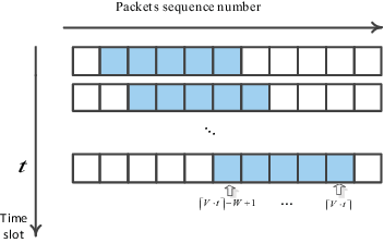
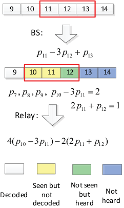
Motivated by these techniques, we propose the MWNC scheme to combine the advantageous features of traditional network coding schemes[25]. MWNC adopts the encoding strategy similar to RLNC, but the block of packets to be encoded in each slot is moving forward at a constant speed (see Fig. 1). Specifically, at time slot , a block of packets with the sequence number ranging from to are encoded with random coefficients on a finite field, which are also transmitted with the coded symbol.22 2 is the ceil function to guarantee that the boundaries of the window are aligned to integer values. Note that if , then the block is started from to . After overhearing the coded symbols from the source, the receiver attempts to decode the original packets through Gauss-Jordan elimination approach. A typical example of the decoding process is shown in Fig. 2, in which the Gauss-Jordan Elimination can be performed progressively as the coded symbol arrives and finally the original packets can be retrieved when the reduced matrix has full rank (Fig. 2(b)). Note that represents the target throughput, so it should be within the network capacity.
In Table I, we show an example where the window size and the moving speed . In this example, the source starts by sending the uncoded packets twice in the first two time slots, one of which is lost by the receiver. Then it sends coded symbols with randomly chosen coefficients in the next two slots (since for ), one of which gets received, so the receiver can successfully decode at the forth time slot. From the fifth time slot, a full window of three packets are encoded in each time slot, which is moved forward with the speed of . Note that because there is no feedback mechanism in MWNC, it cannot guarantee reliability. For example, will get lost at the time slot, since it will never be decoded after the window has moved to , even when the client has received the information of and at the time slot. However, we will prove in Section V that the packet loss probability with MWNC drops almost exponentially with the increase of window size.
MWNC has some other interesting properties. Firstly, the decoding opportunity exists in each time slot, therefore it avoids the intrinsic decoding delay problem incurred by RLNC. In addition, the decoding opportunity is balanced between clients with good and poor channel conditions, so none of the clients will be dominated by other clients with better channel conditions. Secondly, the coding coefficient matrix in buffer is very sparse (see Fig. 2) due to the moving window strategy, so the decoding complexity of MWNC is much lower than RLNC. In Section V, we will develop some theoretical models to analyze these properties.


| Time | Sent symbols | Received? | Decoded/Lost | |
| 1 | 1 | – | ||
| 2 | 1 | D: | ||
| 3 | 2 | – | ||
| 4 | 2 | D: | ||
| 5 | 3 | – | ||
| 6 | 3 | – | ||
| 7 | 4 | – | ||
| 8 | 4 | – | ||
| 9 | 5 | – | ||
| 10 | 5 | – | ||
| 11 | 6 | – | ||
| 12 | 6 | L: , | ||
| 13 | 7 | – |
Note that the concept of network coding over a moving window has been considered in [26] and [27]. In [26], RLNC is incorporated with the congestion window in TCP protocol to improve the throughput in the lossy wireless environment. In [27], SlideOR is proposed to encode packets in overlapping window, which can avoid the throughput loss in opportunistic routing. Our scheme differs from these schemes in the following aspects. Firstly, MWNC can achieve better control of the decoding delay and complexity with appropriate settings of the moving speed and window size, while these schemes are best-effort and there is no guarantee for the decoding delay at the receivers. In addition, we develop theoretical models to characterize the reliability, decoding delay and decoding complexity properties of MWNC. Secondly, these schemes rely on the feedback of the receivers to move forward the coding window, which is nontrivial in wireless broadcasting since the ACKs of different receivers have to be carefully scheduled to avoid collision. In addition, even if the reliability of ACKs can be guaranteed, the feedback delay may lead to the degradation of the network throughput[28]. In our scheme, the coding window is moved forward according to a prescribed moving speed , which does not rely on the feedback from the receivers. Of course, should be carefully set to be within the network capacity to avoid overwhelming the receivers, which is not difficult since the link capacity is assumed to be quasi-static. If the network is dynamic, this parameter should be adapted according to the network condition, which however is beyond the scope of this paper.
IV Design of MWNCast
In this section, we propose MWNCast, a cooperative multicast protocol based on the MWNC technique. Before elaborating on the details of the protocol, we briefly introduce the motivation and basic functionality of MWNCast with a simple example.
IV-A Overview of MWNCast
Consider a simple example as shown in Fig. 3(a), which consists of three receivers, the number on each link is the corresponding PRP. For plain broadcast, it is easy to see the capacity of the system is due to the bottleneck receiver , which requires more time to receive the same amount of information as that of clients and . Therefore, some time is wasted for clients and since the information sent by the source is not innovative to these two receivers after they have received the required data. On the other hand, if these two clients have packets that are not received by client , one of them can forward the packets to client on behalf of the source on a different channel using its residual time, while the other client can continue receiving data from the source. Ideally, if clients are assigned to devote and of their time to serve client alternately while spending the rest of their time to receive from the BS, then the maximum achievable throughput for is , and is . Meanwhile, client can receive data alternately from clients when they are active, and from the BS in the rest time, so its achievable throughput is (see Fig. 3(b)), which suggests that the throughput of (packet/slot) can be achieved through this cooperation scheme.
The key to the success of this cooperative strategy is the scheduling of the relay transmissions, that is, to determine which set of relay node should transmit at a specific time slot. To this end, we adopt a stochastic scheduling method, which works as follows. At the beginning of each time slot, the source generates a random variable uniformly distributed in . If , then is selected to relay the data to , while keeps receiving from the source. If , the roles of and are exchanged. Otherwise, only the source transmits and all clients receive information from it. This scheduling decision is broadcasted to all relays. Each second-hop receiver always receives from the best transmitter (the source or a relay). An example of the scheduling sequences is shown in Fig. 3(c).
The source and the selected relays will transmit at the scheduled time slot. The packets to be transmitted are encoded using the MWNC technique, which range from to at time . The source transmits the encoded symbol on its channel, while the selected relay node transmits a specific encoded symbol on a different channel. For relay node, this encoded symbol is generated from a batch of packets (the most close to the expected window in the relay’s buffer), including the newly decoded packets and the combination of undecoded packets (e.g., , , and in Fig. 3(d)). After overhearing the transmissions from the source and the relay, the end receiver attempt to decode the original packets with Gauss-Jordan elimination technique.


IV-B MWNCast Protocol
In this subsection, we discuss the details of MWNCast protocol. We have explained how to implement MWNC in a cooperative scenario, so in the following we focus on the cooperative scheduling in MWNCast, which can be decomposed into three modules, namely the selection of relay nodes, the allocation of relay time, and the online scheduling of relay transmissions.
IV-B1 Relay node selection
The ultimate goal of MWNCast is to alleviate the bottleneck and maximize the multicast capacity through the cooperation of relays. To this end, we propose a procedure to search for a set of candidate relay nodes that can achieve the maximum capacity. The basic idea is as follows. For a given target network capacity , we can partition the set of receivers into two groups according to the PRPs from the source to these nodes, then the nodes with PRPs above will be selected as the relay nodes since their residual capacities can be used for serving the remaining end receivers.
The rational for selecting relay nodes in this way is that the selected relay nodes can meet the target capacity requirement. However, it cannot guarantee that the remaining nodes can achieve the target capacity as well, since their achievable throughput depends on their link capacities to the relay nodes, as well as how much residual time of these relay nodes can be devoted for cooperation. Therefore, it is necessary to check the feasibility of this target , which involves the computations of the available cooperation time for a given set of relays (to be discussed), with which we can compute the achievable throughput for each receivers. If any of the nodes fail to achieve the target capacity , then it means that this target capacity is infeasible and a smaller value should be attempted, otherwise a larger capacity can be supported.
Based on this idea, we propose a binary search procedure to find the maximum achievable capacity as shown in Algorithm 1. The algorithm maintains a lower threshold and an upper threshold for the target capacity initially. Then starting with , a set of relay nodes with qualified link capacities are determined (lines 5-6). The achievable capacities of the remaining nodes are computed using Algorithm 2 (line 7). If the target capacity can be achieved by all nodes, then the lower threshold is increased to (line 9), otherwise the upper threshold is reduced to (line 11). The same procedure is repeated until the upper and lower thresholds converge. Finally, the algorithm returns the set of qualified relay nodes for the maximum achievable capacity .
IV-B2 Relay time allocation
As discussed in the previous subsection, for a target capacity , if a node has a PRP of , it is selected as a candidate relay node. In this case, at least a fraction of its time has to be used for receiving data from the source so that the target capacity requirement can be satisfied. As a result, its residual time is at most , which can be used for serving the remaining receiver nodes. Therefore, the next problem is to find the allocation of the relay time for each relay node under its residual time budget, such that the target capacity requirement of the end receiver nodes can also be satisfied. If such time allocation exists, it means the target capacity is achievable, and vice versa.
To this end, we propose a relay time allocation algorithm as shown in Algorithm 2, which proceeds in round as follows. In the beginning, each candidate relay node is initialized with the residual time (line 2), and each end receiver node has a residual capacity demand (line 3). In each round , a greedy algorithm (algorithm 3) is invoked to select a subset from with at most elements, such that the overall capacity of all receivers in is maximized (line 7). The capacity of a node is determined as , whereby is the node in that provides the maximum capacity to node among all nodes in .
Given the relay subset , the next step is to decide the time ratio that they can devote for relaying. Note that since none of the relay nodes should contribute more than its residual time, and none of the receiver nodes should get service more than its residual capacity demand, so the rely time for this subset is set to the minimum of the residual time of these relay nodes and the residual demand of all receivers (line 8), then for each selected relay node , its residual time is reduced by the amount of (line 10). If its residual time is used up, it is removed from the candidate relay set and will not participate in the relay time allocation in the next round (line 11). Similarly, for each receiver , its residual demand is reduced by an amount of , which is the effective throughput it will receive from this set of relay nodes (line 14). If its demand is satisfied, it is removed from receiver set and will be considered in the next round (line 15). The same procedure is repeated to find the next subset of relay nodes and its relay time allocation, until either the candidate relay set or the receiver set becomes empty, or the overall relay time reaches 1 (line 8). If the receiver set is empty eventually, it means that the target capacity demand can be met by all receiver nodes, then the algorithm returns a list of relay subsets and their corresponding relay time; Otherwise, it means the target capacity is infeasible and the algorithm returns an empty set.
In each round of Algorithm 2 (line 7), we need to find a subset of at most relay nodes that can provide maximum capacity to the unsatisfied receivers together with the source node. Let denote the set nodes consisting of the candidate relay set and the source node . The capacity of a selection of relay nodes is defined as . Our objective is to find a selection with the maximum capacity such that the . This problem is known as a special case of the generalized maximum coverage problem, which is NP-hard [29]. To solve this problem, we introduce the following definitions:
Definition 1.
(residual capacity/weight) Consider a selection , a relay and a receiver . We define the residual capacity to be equal to .
Definition 2.
(addition of a relay) For a selection and a relay , we define as the addition of to . In other words, is a new selection , and
Base on these concepts, we develop a greedy algorithm as shown in Algorithm 3. The basic idea is to incrementally add the relay node with the maximum positive residual capacity, so that the overall capacity is non-decreasing. At line 3, all receivers are initially assigned to the source. Then in each round, one of the candidate relays that has the maximum positive residual capacity is selected to join the relay node set (line 6) until exceeds . It can be proved that this greedy algorithm can achieve an approximation ratio of to the optimal solution [29].
IV-B3 Online Relay Transmission Scheduling
From Algorithms 1 and 2, we can find a list of relay node set and the corresponding relay time allocation , such that the multicast capacity of the system is maximized. Let denote the maximum capacity corresponding to the results, then for any capacity requirement , we should have:
| (4) |
From (4), we can see that the amount of time that a subset to be scheduled for relaying should be proportional to , such that the required capacity can be satisfied. Since the time is slotted, as briefly introduced in last section, we can adopt a stochastic online algorithm to approximate the scheduling. Specifically, let us define as
| (5) |
In each time slot , the source generates a random number between 0 and 1, if its value falls between and , then the subset of relay nodes are selected for relaying in this time slot. It is easy to see that this stochastic scheduling policy converges to the required proportional of time for each relay set in a long run. This schedule algorithm can be executed by the source in an online fashion at the beginning of each time slot, and an unique channel is assigned to each selected relay node. The scheduling results (relay nodes and their operating channels) are broadcasted to all receivers, then they can choose the best relay node and switch to the corresponding channel to receive the data.
V Analysis
In this section, we develop some theoretical models to characterize the basic properties of MWNCast. Firstly, we introduce the equivalent channel capacity model, which is an unified model for characterizing the capacity of both relay and receiver nodes. Based on this model, the decoding delay, reliability and decoding complexity properties of MWNCast are analyzed using the random walk and point process theories.
V-A Equivalent Channel Capacity Model
As discussed in Section II, the capacity of a point-to-point wireless link is given by the PRP . However, the analysis of the link capacity in MWNCast is complicated since: (i) a relay node may not stay in the “receiving” state all the time; (ii) a receiver node may receive data from different relay nodes at different time slots. In this subsection, we propose an equivalent channel capacity model to characterize the capacity of these two kinds of nodes.
For a relay node , its aggregated fraction of time in the “relaying” state is given by . Since the online relay scheduling algorithm is a stochastic scheme, we can assume that in each time slot, the probability for the node to receive from the source is , and the probability for relaying is . Taking into account the PRP from the source, we can define the equivalent channel capacity for this relay node as , which is the maximum achievable throughput of this node from the source without errors.
For a receiver node , if a relay subset is selected for transmission (with a probability of ), it will choose to receive from the best relay node (including the source) with the maximum PRP, i.e., . Therefore, we can define the equivalent channel capacity for node as the aggregated throughput from all relay subsets, i.e., .
Note that this equivalent channel capacity model is an approximation of the link capacity for the two kinds of nodes in MWNCast, which makes it tractable to analyze the reliability and decoding delay properties in the following subsections.
V-B Preliminary Property of MWNC
In this subsection, we establish some basic properties for MWNC using the random walk and point process theories, with which we can analyze the performance of MWNCast.
In the following, we use the “packet” to denote the original data, and the “symbol” to denote the linear combination of the packets within the window. For any receiver with capacity , let us define as the number of packets which are inevitably lost up to time , as the total number of received innovative symbols up to . Note that not all innovative symbols can be used for decoding the original packets. For example, in Table I, the symbol received at is useless at the end of time since cannot be decoded ever since. We define as the number of discarded symbols up to time . Then represents the received innovative symbols that contain the information for the packets covered by the coding window up to time (except for the lost packets).
For a MWNC’s receiver with capacity , let us define a particle on with its position at time given by
| (6) |
We have the following results regarding the decoding and loss events for MWNC.
Lemma 1.
Decoding event occurs at time if and only if at the end of this time slot. All the packets from the last foremost decoded (or lost) packet to the head of current window will be decoded.
Proof.
Decoding event occurs at the moment when the coding coefficient matrix in buffer is full rank. In this case, the number of innovative symbols in buffer must be as many as the number of packets covered by the window by time except for the lost ones, i.e., . Therefore, we have , i.e., . ∎
Lemma 2.
Packet loss event occurs at time if and only if at the end of . Moreover, all the un-decoded packets before the tail of the window are lost.
Proof.
The last packet in the coding window moves to at time . So if the packet right before has not been “seen” (i.e., a symbol contains this packet has not been received before), then all the un-decoded packets before the window will get lost forever. In other words, , which gets . ∎
Lemma 3.
If a new packet is lost at time , the number of newly discarded symbols in buffer must be exactly one less than the number of packets just get lost, i.e.,
| (7) |
Proof.
Since the coding window moves constantly, if the packet has not been “seen” at time , then the packet should have been decided as lost in the last time slot, which contradicts to the assumption. ∎
Accordingly, for the specified receiver, MWNC can be modeled as a one-dimensional random walks [30] (see Fig. 4). The random walk has two reflecting barriers at and corresponding to the decoding and packet loss events respectively, where in (6) corresponds to the position of the random walk at time . Let denote the step size of the random walk, which is a random variable with the following density function:
| (8) |
where and . Moreover, the mean and variance of a step are denoted as and .

The following theorem specifies the behavior of the random walk representing the specified receiver:
Theorem 1.
At time , if the particle crosses the left barrier , it will be reflected rightward for a distance of in the next time slot. If the particle crosses the right barrier , it will be immediately bounced back for a distance of . Otherwise, the particle will make a random move according to (8).
Proof.
Firstly, notice that if and only if , the received symbol at time is innovative. That is, the window’s foremost packet is informative to the receiver since .
Therefore, when the particle does not cross the two barriers, its position at time relative to the last slot depends on whether a symbol is received successfully, which follows the the step function defined in (8). If the particle just crosses the left barrier , the received symbol contains no new information. Thus and the particle moves rightward definitely. If the particle crosses the right barrier , it is indicated in Lemma 3 that it will be bounced back instantly by a distance of . ∎
V-C Reliability Analysis
The reliability analysis is complicated in MWNCast since the second-hop receivers might suffer from larger packet loss ratio. However, it is easy to see that the proposed stochastic scheduling policy converges to the required proportional of time for each relay set in a long run and consequently the information difference between BS and the relays should not be large. In addition, the symbols to be transmitted by the relays are generated randomly, so that the probability that they contain innovative information to the second-hop receivers is greatly increased. Therefore, without differentiating the relays and receivers, we assume a specified client receives information on a channel of equivalent capacity . Based on this assumption, the packet loss ratio for both the relays and the receivers can be derived.
We can model MWNCast as a two-state point process [30] as shown in Fig. 5, which corresponds to the “Decode” (D) and “Loss” (L) events, respectively. Specifically, if the “Decode” event occurs at some time, with probability it will return the same state after a random time interval , and with probability it will make a transition to the “Loss” states after a time interval . Similarly, we can define and as the transition probabilities and transition time for the “Loss” state. These quantities can be derived using the random walk and point process theories as follows.

Firstly, let us define as the moment generating function of , which is the two-sided Laplace transform of the step function defined in (8), that is,
| (9) |
From the property of moment generating function, we know that: (i) is a convex function; (ii) If , there are two roots for the equation , one is , the other is who has the same sign as .
Let and () denote two absorbing barriers for the random walk starting at the origin, we can define the stopping time as
| (10) |
which is the number of steps to cross one of the barriers starting from the origin.
We can define the moment generating function with respect to and , that is,
| (11) |
Suppose that we set , then we have . For this equation, we can find such that , then it is easy to verify that is a martingale with mean 1 since it is the product of independent unit mean random variables. According to the martingale stopping theorem (Theorem 6.2.2 in [31]), we can obtain:
| (12) |
Since the events of and are independent, from (10) and (12), we have:
| (13) |
For the absorbing states and , we can get the following approximations:
Substituting these two approximation equations into (12), and using the fact that , we can get the probabilities of absorption at and as
| (14) |
where is the non-zero root of the equation .
To derive the distribution for , let and denote two real roots of the equation . Then from (11), we can obtain a different expression of (12) with respect to :
| (15) |
Using the approximation when , and when , we have:
| (16) |
where and denote the conditional expectations at and , respectively. Using and given by (14), we can obtain and from (16). Then we have the moment generating function for as:
| (17) |
By differentiating Eq. (17) with respect to , we can obtain the first and second moments of respectively.
To derive the packet loss ratio, we assume the particle is always located at the largest possible position after an event, which gives the upper bound for the loss probability. By Theorem 1, after an “D” event, the particle’s maximum position is at ; After a “L” event, the particle must get back to at most before making a random move. Therefore, the transition probabilities and between these two events, and the expected transition time and can be derived using (14) and (17) respectively assuming the particle starting from the corresponding position.
The equilibrium distribution of the embedded Markov chain for two-state point process can be given by . Let us define , then the proportion of time passed from states “L” and “D” to state “L” are given by and , respectively.
Note that MWNC has two packet loss scenairo depending on the previous event, “L” to “L” and “D” to “L”. If it is from “L” to “L”, all the packets covered by the window will get lost, so the number of lost packets should be proportional to the transition time . If it is from “D” to “L”, then the lost packets should be the number of packets covered from the time of previous event minus since only the packets behind the window will get lost. Therefore, the overall packet loss probability can be obtained as:
| (18) |
V-D Decoding delay analysis
For a receiver in MWNCast, the delay for receiving a packet is composed of two parts: the queueing delay and the decoding delay. The queueing delay can be analyzed using the similar procedure in [18]. In the following, we will focus on the decoding delay and consider a saturated system in which the source always has packets to transmitted.
Attributed to the stochastic scheduling policy, any client (a relay or a receiver) in the network can be approximately considered as connected to the information source by MWNC on a channel with equivalent capacity . If the window size is sufficiently large, the packet loss probability is negligible. In this case, we can derive an upper bound for the average decoding delay assuming that , whereby the random walk is simplified to a single left barrier at with a starting point . The barrier at indicates the moment of decoding. Assume the particle always reflects back to the largest possible position after a decoding event. According to Eq. (17), when approaches to infinity and is set , we have and . The first two moments of are derived from (17) as follows:
| (19) |
The decoding delay for a packet is defined as the time duration from the moment that it is encoded to the time that it is decoded. We can model the decoding process as a renewal process. Then the sum of decoding delay for the packet in a renewal period is given by
where is the average decoding delay for a packet, is the average number symbols transmitted during this time period.
By the theory of renewal reward process and the definition of average decoding delay, we have
| (20) |
V-E Decoding Complexity
In this part, we analyze the decoding complexity of MWNC assuming the window size is sufficiently large such that the packet loss can be negligible.
The decoding complexity of MWNC is composed of two parts: the forward elimination and the backward substitution. Suppose that a receiver has just decoded all packets up to at time , and denote the time instances that the receiver receives a set of encoded symbols but cannot decode them, until at time it receives the th symbol and is able to decode all the received symbols. In the following, we use to denote the symbol received at time .
Lemma 4.
The number of nonzero entries in the symbol after the forward elimination is .
Proof.
The forward elimination can assure that all the previously “seen” packets can be reduced from the newly received symbol. At time , the receiver has received useful symbols. Hence, except for inevitably lost ones, all the packets up to have been “seen” even they may not be all decoded. The new symbol generated in the ’s coding window can be reduced at the corresponding positions except for the last one , which becomes “seen” for the sake of the symbol received at . Hence, there are nonzero entries are left, which equals to according to Eq. (6). ∎
Lemma 5.
The number of arithmetic operations required for forward elimination of the symbol is when , and otherwise.
Proof.
The packets from to are used to generate the specific symbol. Among them, the receiver may have decoded a number of packets. Since as Lemma 4 suggests, the number of nonzero entries after elimination is and there are previously eliminated results, the receiver only has a decoded intersection with the coding window if . In this case, the first packets in the window are already decoded by the receiver, so the same number of calculations are needed to eliminate these entries. Then, the previously reduced symbols () can be used to eliminate the corresponding entries, which takes operations for each symbol according to Lemma 4. When , there are no decoded packets in the coding window, thus the receiver can only use the existing eliminated results to reduce the symbol. The elimination for the positions takes calculations. ∎
Theorem 2.
Given the target throughput , MWNC can achieve the optimal decoding complexity of .
Proof.
A network coding symbol is encoded with packets, a receiver needs at least operation to decode the original information, so a trivial lower bound for the decoding complexity is . Therefore, it is sufficient to prove that, for every receiver in the network, the decoding complexity of MWNC is upper bounded by .
According to Lemma 5, an obvious upper bound of complexity for the symbol’s elimination procedure is 33 3 For , the first symbol certainly needs no more than operations, thus without abusing the notation, we assume .. Thus, the total number of computations for the forward elimination of packets is upper bounded by . The total number of computations for backward substitution is , so the overall complexity for decoding packets is bounded by:
| (21) |
where the second inequality is valid because .
Note that as discussed in previous subsection, the decoding event occurs after a random time duration of , so . According to the renewal reward process and (21), the average decoding complexity can be obtained as follows:
| (22) |
VI Simulation Results
In this section, we provide extensive simulation results to compare the performance of MWNCast with other network coding-based multicast schemes, and also to illustrate the advantages of MWNC technique. The network topologies in simulations are generated randomly, whereby the location of all clients is uniformly distributed around the source. The channel between any two nodes is assumed to follow the Rayleigh fading channel model. The coefficients of network coding are generated on a Galois Field. The time duration for each simulation is time slots.
VI-A Throughput and Decoding Delay
In Fig. 6, we compare the achievable throughput of MWNCast44 4 The packet loss probability is controlled under as will be explained in the next subsection. with those of RLNC and ANC under different network sizes, where the window size of MWNCast is set to . When the channel number , MWNCast reduces to MWNC (simple multicast without cooperation). We can see that the achieved throughput of MWNC is close to ANC (which is known to be throughput-optimal), but it outperforms RLNC under all network conditions. It also can be seen that the throughput of RLNC decreases as the network size increases, which has been discussed in the literature [14]. When multiple channels are available, we provide the simulation for RLNC with the same relay scheduling strategy as in MWNCast for fair comparison. It is observed that for and , MWNCast preserves its superiority over cooperative RLNC (denoted by CoopRLNC in Fig. 6) with the average performance gain of and , respectively. Therefore, we can see that by taking advantage of moving window network coding and cooperation, MWNCast is effective in improving the system throughput.
In Fig. 7, we study the tradeoff between the decoding delay and throughput for a network with 100 nodes. Note that the result of ANC is not included since the decoding delay of the receivers with poorer channel condition increases with the simulation time, which is unfair for comparison. In this figure, the lines and bars show the average and maximum decoding delays of all receivers respectively for each scheme. It is noteworthy that, to maintain a given throughput, with the newly proposed MWNC-based scheme, the average decoding delay for a successful decoded packet is much lower than that with the RLNC-based scheme. The reason is that the decoding opportunity with MWNC exists in each time slot, but with RLNC, it cannot decode until receiving the full block of packets.
VI-B Reliability
In Fig. 8, we study the effect of window size on the packet loss ratios of MWNCast under different system traffic load conditions 55 5 System traffic load is defined as . when the channel number . The packet loss counted in the simulation can occur at any clients in the network. From the figure, it can be seen that the theoretical results match well with the simulation results. Also, we notice that, the packet loss probability drops almost exponentially with the increase of window size. Moreover, we can see the requirement of packet loss probability of can be satisfied with even when the traffic load is as high as .
If a certain degree of packet loss can be tolerated (i.e. ), we study the relationship between the average decoding delay and packet loss probability by adjusting the window size. We consider a specific receiver with the packet erasure probability equals to . As shown in Fig. 9, for a given traffic load, the packet loss probability increases with the decrease of window size, but the average decoding delay for the packets not lost also gets smaller. As discussed in Lemma 2, this is because packet loss is inevitable when and only when the the last unseen packet is just the one before the lattermost packet in the window. Such packets, if not lost, will encumber the decoding of the following packets, leading to larger overall decoding delay. Therefore, with a smaller coding window size, MWNCast acts as a delay filter to force the receiver to drop the packets which may lead to the degradation of the overall delay performance.
VI-C Decoding Complexity
In Fig. 10, we compare the decoding complexity of MWNC and RLNC. It can be seen that the decoding complexity of MWNC is much smaller than that of RLNC. It is found that to decode RLNC, the forward elimination is the dominating part (i.e., ) as increases and hence the average complexity for decoding an original packet is . Nevertheless, in order to achieve higher throughput, larger batch sizes have to be used, so the decoding complexity of RLNC increases dramatically with the growing of throughput. For MWNC, the decoding coefficient matrix of the receiver is sparse since it has smaller number of non-zero items. As a result, the decoding complexity consumed by Gauss Elimination is significantly reduced (proportional to the window size) and has little dependency on the throughput.


VII Conclusions
In this paper, we proposed MWNC, a novel network coding scheme that has smaller decoding delay, lower complexity and no need for feedback from the receivers. Based on this technique, we further present the MWNCast protocol to address the bottleneck problem in wireless multicast through cooperative relays. Theoretical analysis shows that the proposed schemes can approach the network capacity with the packet loss probability dropping almost exponentially with the increase of window size, the average decoding delay is on the order of and the decoding complexity is on the order . Simulation results are provided to validate the theoretical results and compare the performance of the proposed schemes with the existing solutions.
References
- [1] F. Wu, C. Hua, H. Shan, and A. Huang, “Mwncast: cooperative multicast based on moving window network coding,” in IEEE GLOBECOM’12, pp. 1–7, 2012.
- [2] G. Papadopoulos, G. Koltsidas, and F. Pavlidou, “Two hybrid arq algorithms for reliable multicast communications in umts networks,” IEEE Communications Letters, vol. 10, no. 4, pp. 260–262, 2006.
- [3] X. Zhang and Q. Du, “Adaptive low-complexity erasure-correcting code-based protocols for qos-driven mobile multicast services over wireless networks,” IEEE Transactions on Vehicular Technology, vol. 55, no. 5, pp. 1633–1647, 2006.
- [4] M. Luby, “LT codes,” in Proceedings of the IEEE Symposium on the Foundations of Computer Science, pp. 271–280, 2002.
- [5] A. Shokrollahi, “Raptor codes,” IEEE/ACM Trans. on Networking, vol. 14, pp. 2551–2567, June 2006.
- [6] T. Ho, Networking from a network coding perspective. PhD thesis, MIT, 2004.
- [7] O. Alay, P. Liu, Z. Guo, L. Wang, Y. Wang, E. Erkip, and S. Panwar, “Cooperative layered video multicast using randomized distributed space time codes,” in IEEE INFOCOM Workshops, pp. 1–6, 2009.
- [8] B. Rong and A. Hafid, “Cooperative multicast for mobile iptv over wireless mesh networks: The relay-selection study,” IEEE Transactions on Vehicular Technology, vol. 59, no. 5, pp. 2207–2218, 2010.
- [9] H. Zhao and W. Su, “Cooperative wireless multicast: performance analysis and power/location optimization,” IEEE Transactions on Wireless Communications, vol. 9, no. 6, pp. 2088–2100, 2010.
- [10] P. Fan, C. Zhi, C. Wei, and K. Ben Letaief, “Reliable relay assisted wireless multicast using network coding,” IEEE Journal on Selected Areas in Communications, vol. 27, no. 5, pp. 749–762, 2009.
- [11] J. Jin and B. Li, “Cooperative multicast scheduling with random network coding in wimax,” in 17th International Workshop on Quality of Service (IWQoS’09), pp. 1–9, 2009.
- [12] A. Fanous and A. Ephremides, “Network-level cooperative protocols for wireless multicasting: Stable throughput analysis and use of network coding,” in IEEE Information Theory Workshop (ITW), pp. 1–5, 2010.
- [13] D. Koutsonikolas, Y. C. Hu, and C.-C. Wang, “Pacifier: High-throughput, reliable multicast without crying babies in wireless mesh networks,” IEEE/ACM Transactions on Networking, vol. PP, no. 99, p. 1, 2011.
- [14] B. Swapna, A. Eryilmaz, and N. Shroff, “Throughput-delay analysis of random linear network coding for wireless broadcasting,” in NetCod’10, June 2010.
- [15] S. Chachulski, M. Jennings, S. Katti, and D. Katabi, “Trading structure for randomness in wireless opportunistic routing,” SIGCOMM Comput. Commun. Rev., vol. 37, pp. 169–180, Aug. 2007.
- [16] J. Padhye, S. Agarwal, V. N. Padmanabhan, L. Qiu, A. Rao, and B. Zill, “Estimation of link interference in static multi-hop wireless networks,” in Proceedings of the 5th ACM SIGCOMM conference on Internet Measurement (IMC’05), pp. 28–28, 2005.
- [17] C. Reis, R. Mahajan, M. Rodrig, D. Wetherall, and J. Zahorjan, “Measurement-based models of delivery and interference in static wireless networks,” in SIGCOMM ’06, pp. 51–62, 2006.
- [18] J. Kumar Sundararajan, D. Shah, and M. Medard, “Arq for network coding,” in IEEE ISIT’08, pp. 1651 –1655, July 2008.
- [19] W. Yeow, A. Hoang, and C. Tham, “Minimizing delay for multicast-streaming in wireless networks with network coding,” in IEEE INFOCOM’09, pp. 190–198, 2009.
- [20] J. Sundararajan, D. Shah, and M. Médard, “Online network coding for optimal throughput and delay-the three-receiver case,” in International Symposium on Information Theory and Its Applications (ISITA’08), pp. 1–6, 2008.
- [21] J. Barros, R. Costa, D. Munaretto, and J. Widmer, “Effective delay control in online network coding,” in IEEE INFOCOM’09, pp. 208 –216, April 2009.
- [22] S. Sorour and S. Valaee, “Minimum broadcast decoding delay for generalized instantly decodable network coding,” in IEEE GLOBECOM’10, pp. 1–5, 2010.
- [23] L. Keller, E. Drinea, and C. Pragouli, “Online broadcasting with network coding,” in Fourth Workshop on Network Coding, Theory and Applications (NetCod’08)., pp. 1–6, 2008.
- [24] I. Hou, P. Kumar, et al., “Broadcasting delay-constrained traffic over unreliable wireless links with network coding,” in Proceedings of the Twelfth ACM International Symposium on Mobile Ad Hoc Networking and Computing, p. 4, 2011.
- [25] F. Wu, C. Hua, H. Shan, and A. Huang, “Reliable network coding for minimizing decoding delay and feedback overhead in wireless broadcasting,” in IEEE PIMRC’12, pp. 1–6, 2012.
- [26] J. Sundararajan, D. Shah, M. Médard, M. Mitzenmacher, and J. Barros, “Network coding meets tcp,” in IEEE INFOCOM’09, pp. 280–288, 2009.
- [27] Y. Lin, B. Liang, and B. Li, “Slideor: Online opportunistic network coding in wireless mesh networks,” in IEEE INFOCOM’10, pp. 1–5, 2010.
- [28] G. Wang, X. Zhao, and X. Dai, “On efficient network coding scheme with lossy and delayed feedback,” in 2011 International Symposium on Network Coding (NetCod), pp. 1 –6, july 2011.
- [29] R. Cohen and L. Katzir, “The generalized maximum coverage problem,” Inf. Process. Letter, vol. 108, pp. 15–22, September 2008.
- [30] D.R.Cox and H. Miller, Theory of Stochastic Processes. Methuen, London, 1965.
- [31] S. M. Ross, Stochastic Processes. John Wiley & Sons, 1996.