Systematic experimental exploration of bifurcations with non-invasive control
Abstract
We present a general method for systematically investigating the dynamics and bifurcations of a physical nonlinear experiment. In particular, we show how the odd-number limitation inherent in popular non-invasive control schemes, such as (Pyragas) time-delayed or washout-filtered feedback control, can be overcome for tracking equilibria or forced periodic orbits in experiments. To demonstrate the use of our non-invasive control, we trace out experimentally the resonance surface of a periodically forced mechanical nonlinear oscillator near the onset of instability, around two saddle-node bifurcations (folds) and a cusp bifurcation.
Keywords:
experimental bifurcation analysis, non-invasive control, odd-number limitationpacs
05.45.Gg,45.80.+r,02.30.OzFeedback control is not only of interest as a tool for system manipulation in the classical control engineering sense, but it can also be used for model verification and discovery, if one can ensure that it is non-invasive. Washout-filtered feedback and Pyragas’ time-delayed feedback (TDF) are popular feedback control schemes that are automatically non-invasive [1, 2]. For example, TDF feeds a signal back into the experimental dynamical system, where is some system output (possibly processed), is a vector or matrix of control gains and is an a-priori chosen time delay. If the time delay equals the period of a periodic orbit () of the uncontrolled dynamical system and the gains are such that the control is stabilizing, then the controlled system will also have the periodic orbit , because the control input vanishes for all time (that is, the control becomes non-invasive). However, the control has changed the stability of , making it visible in the experiment.
While sometimes TDF (or its extended version [3]) is used for engineering purposes (suppression of period doublings leading to chaos [4, 5]), non-invasiveness is not essential in these applications. Thus, in these cases the delayed term in the feedback loop could have been replaced by a periodic reference signal approximately resembling the desired behaviour. TDF draws interest mostly in the scientific community because it enables experimenters to explore dynamical phenomena such as equilibria and periodic orbits of the original uncontrolled system regardless of their dynamical stability [6, 7, 8, 9, 10, 11].
Systematic studies that try to explore the parameter space of the uncontrolled system and that use TDF or washout filters to stabilize equilibria and periodic orbits non-invasively encounter a major difficulty: it is not known under which conditions one can find control gains that successfully stabilize a periodic orbit [12]. This is in contrast to classical feedback control where one feeds with a pre-determined reference signal back into the system. For classical feedback control it is known that, if corresponds to an equilibrium or periodic orbit of the uncontrolled system then, under some genericity assumptions (controllability and observability), one can always locally stabilize the equilibrium or periodic orbit even if it has arbitrarily many unstable eigenvalues [13]. Experimental and theoretical studies have explored the limits of applicability of TDF and restrictions on the gains due to instabilities caused by the TDF feedback term [11, 14, 15, 16]. In particular, there are topological restrictions (the odd-number limitation [17, 18]) which guarantee that TDF cannot possibly work in some of the most common cases. One common scenario where it would be natural to use TDF is ruled out by the odd-number limitation: an equilibrium of an autonomous system or a periodic orbit of a periodically forced system in the vicinity of a system parameter setting where it makes a fold (called saddle-node bifurcation, see Fig. 1 for a typical bifurcation diagram). Even the unstable controller proposed in [19] fails to stabilize uniformly near the fold.
In this paper, we present a simple alternative approach to exploring bifurcation scenarios, including the unstable branches. Our approach exploits the fact that the goal of the experiment is a parameter study in a system parameter , rather than finding a single equilibrium or periodic orbit at a specified parameter value. It is applicable whenever the feedback control is achieved by (effectively) varying the same system parameter that one wants to use for the bifurcation diagram.
Finally, we illustrate the power of this approach by tracking branches of periodic orbits in a physical experiment to produce a solution surface that shows two fold curves meeting at a cusp bifurcation.
I Steady-state branch tracking
We first explain the basic approach applied to tracking a branch of equilibria in the case of a single-input single-output system. A stable and an unstable branch, connected by a fold, are traced out as a function of the system parameter. We then generalize the approach to the case of tracking periodic orbits and show its application in an experimental setting. As our method does not rely on knowledge of the state of the model we do not distinguish between state and output, calling the output .
I.1 Equilibria
Suppose that we have an experiment with a scalar output and a scalar system parameter , which has a bifurcation diagram for its equilibria as illustrated in Fig. 1: a stable and an unstable branch of equilibria meeting in a fold (saddle-node bifurcation). We assume that we can use the parameter as a (scalar) control input such that control is added to the parameter . Consider what happens if we pick a point in the -plane and apply a simple proportional feedback controller of the form
| (1) |
where is the control gain (see Fig. 1). The linear relation (1) restricts the dynamics of the experiment to move along the tilted dashed line in Fig. 1. The equilibria of the feedback-controlled system are the intersections of this tilted line with the curve of equilibria in the -plane. In Fig. 1 this intersection point is . Close to the fold and for sufficiently small the underlying dynamics is one-dimensional such that the intersection point corresponds to a stable equilibrium of the experiment with feedback control (1) (and, at the same time, to a possibly unstable equilibrium of the uncontrolled system).
This simple trick illustrated in Fig. 1 permits one to trace out branches of equilibria around folds with a continuation procedure. Assume that we have already found two equilibria and along the branch, and that the experiment is currently at equilibrium . First we use a secant approximation to generate a prediction for the next equilibrium, which gives
| (2) |
where in Fig. 1. (The prediction step can be chosen adaptively to ensure the desired resolution of the equilibrium branch.) Then the experiment is run with the feedback control (1) based on the point determined by (2). Once the transients have settled to a constant value, the next equilibrium along the branch is given by
Then we can repeat the procedure by picking the next prediction using (2) for index , finding the next equilibrium along the branch.
Figure 1 also illustrates the dynamics of the system after one sets the feedback control to (1) with (2). The system parameter and the control input adjust immediately such that initially jumps rapidly in horizontal direction (thick light gray line with double arrows in Fig. 1). Then the system follows the dynamics imposed by the feedback control (1) along the tilted line given by (1), gradually settling to its equilibrium (thick light gray line with single arrow in Fig. 1).
The approach illustrated in Fig. 1 is non-invasive: every equilibrium of the feedback controlled system corresponds to an equilibrium of the uncontrolled system and a-priori knowledge of the equilibrium of the uncontrolled system is not necessary.
I.2 Periodic orbits
For our demonstration experiment, which is periodically forced, we need to generalize the approach to enable it to trace periodic steady states of periodically forced systems with proportional-plus-derivative (PD) control. Here the input parameter is harmonic forcing, that is,
This allows for an arbitrary phase shift in the forcing and simplifies the method below. We perform a parameter study in the forcing amplitude . Mimicking the approach of Fig. 1, we pick a harmonic forcing amplitude
| (3) |
(playing the role of in Fig. 1) and an arbitrary periodic reference signal (expanded to finitely many Fourier modes)
| (4) |
(playing the role of in Fig. 1), and apply the PD feedback law (an idealized version of what we do in the experiment in section III)
| (5) |
where is the output of the system. Assuming that the PD control is stabilizing, the system will settle into a periodic steady-state output (also expanded to Fourier modes):
| (6) |
We notice that the experiment with feedback control (5) also has periodic input after the transients have settled (the right-hand side of (5) is periodic for periodic and ). The amplitude of the forcing at the fundamental frequency equals , where
| (7) | ||||
However, the forcing is not purely harmonic asymptotically due to the presence of nonlinearities. Even if the reference signal is harmonic, the output will not be harmonic because of the nonlinearities of the experimental system. The non-harmonic Fourier coefficients of are
If these are zero then the forcing will be harmonic with amplitude such that the point will be on the branch of periodic orbits. The requirement for to be zero is a nonlinear system of equations for the non-harmonic Fourier coefficients of the reference signal (which are variables). This nonlinear system can be written as a nonlinear fixed-point problem:
| (8) | ||||
The output (and, thus, its vector of non-harmonic Fourier coefficients ) also depends on the harmonic amplitudes and , which act as parameters in (8) but were omitted as arguments in (8). In general the fixed-point problem (8) has to be solved with a Newton iteration (this is what [20, 21, 22, 23, 24] do for all Fourier coefficients). However, in many practical experiments it may be sufficient to apply a simple fixed point iteration to the fixed-point problem (this is the approach we take in section III):
| (9) |
Algorithm
In summary, the procedure to find a new periodic orbit on the branch looks as follows. Assume that we have found already two previous points along the branch of periodic orbits, namely and . The inputs and are harmonic and the outputs and are periodic. We use a secant approximation to generate a prediction for the next solution point, which gives
| (10) |
(again by default, but can be chosen adaptive). We set and , and repeat the following procedure until convergence.
- 1.
Run the experiment with PD feedback law (5) and and as given. Wait until the experiment settles to a periodic output .
- 2.
- 3.
Check if the root-mean-square error
is smaller than the desired tolerance. (Note that the index is skipped in the sum!) If yes, finish the iteration. Otherwise, set
set the reference signal to these new non-harmonic Fourier coefficients according to (4) (keeping and as before), and repeat from step 1.
After the iteration is finished, the accepted point on the branch is
where is the asymptotic output at the end of the iteration, and and are the harmonic Fourier coefficients of the asymptotic input . The coefficients and are given in (7) but they can also be extracted directly from the input (the input is harmonic up to tolerance after the iteration).
II Discussion of the method
The technique presented in section I.1 is guaranteed to be applicable near folds of equilibria involving one stable branch for single inputs and outputs that give a bifurcation diagram as in Fig. 1. It fails in points where the equilibrium output does not depend on the parameter at the linear level (that is, for example, at transcritical bifurcations or when the branch is horizontal in the -plane). The reason is that the genericity assumption for successful control (stabilizability and observability) is violated in these points.
As the control is applied by varying the bifurcation parameter several parameters are not truly independent. For example, in section I.1 the parameter pair enters only as a combination , such that one can treat them as a single parameter. The same applies to the parameters and , and and in section I.2. Because a continuation of a forced system in the forcing amplitude has effectively two free parameters (the forcing amplitude and the phase), only the overall amplitude needs to be monitored.
The approach presented in sections I.1 and I.2 should be compared with the alternatives for control-based identification of bifurcations suggested in the literature: the detection of the fold bifurcation in [25] required identification of the normal form coefficients. Time-delayed feedback and wash-out filtered feedback are not able to stabilize equilibria uniformly near the fold [26, 27, 1] (also when they are modified by adding degrees of freedom [19]). The general approach proposed in [28] and taken in [20, 21, 22, 23, 24] searches not for the equilibrium on the branch that intersects the line given by the feedback law (1), but finds the equilibrium on a prescribed line perpendicular to the secant through (pseudo-arclength continuation). That is, it sets the feedback law to
| (11) |
and determines by solving the nonlinear system of equations
| (12) | ||||
| (13) |
where is the steady-state output of the experiment with parameter and feedback control (11) after the transients have settled. This pseudo-arclength continuation in [20, 21, 22, 23, 24] required adjustments of in a Newton iteration for system (12), (13) to make the control non-invasive (enforced by (12)) on the line prescribed by (13). In this sense the procedure of Fig. 1 is a simplification of the control-based pseudo-arclength continuation of [20, 21, 22, 23, 24] that can be used whenever the feedback control is applied by varying the bifurcation parameter (which is not the case for [23, 24]).
The method presented in section I promises a substantial speed-up compared to [20, 21, 22, 23, 24] by removing one equation per free bifurcation parameter from the fixed point problem (12), instead of adding the equation (13). The projection onto the solution surface occurs along a line determined by the control gains . Whenever the remaining equations of (12) can be solved by a simple fixed-point iteration (or there are no equations remaining), this removes the need for a full Newton iteration.
The extension to periodic orbits of forced systems proposed in section I.2 applies the method shown in Fig. 1 to the harmonic part and combines it with a simple fixed-point iteration for the non-harmonic part. In general, the simple fixed-point iteration cannot be guaranteed to converge for strongly non-harmonic periodic orbits. If one introduces a relaxation parameter into the iteration (9) (that is, setting ) and chooses small, then the iteration becomes equivalent to the extended time-delayed feedback (ETDF) method [3] to finding periodic orbits (which also has a relaxation parameter), but restricted to the non-harmonic Fourier coefficients. This restriction to the non-harmonic Fourier coefficients is essential. An algorithm updating all Fourier coefficients in step 3 of the description in section I.2 suffers from the same odd-number limitation as the ETDF method.
III Experimental set-up and methods

The demonstration experiment is the forced nonlinear oscillator shown in Fig. 2, an electro-magnetic energy harvester [21, 22], mounted on a force-controlled electro-dynamic shaker also shown in Fig. 2. Due to magnetic hysteresis and eddy currents this system is difficult to characterize with a low number of degrees of freedom in a way that is able to reproduce the experimental bifurcation diagram (see Fig. 5(a)) quantitatively. In particular, one would have to introduce an “effective” damping coefficient that depends on the forcing frequency and the response amplitude and phase [29].
The experimental set-up, shown in Fig. 2, consists of a generic electrodynamic shaker, a Maxon ADS 50/10 current controller and a dSpace DS1104 real-time measurement and control system.
The input to the energy harvester is a force that is directly proportional to the current supplied to the shaker. Thus the current controller enables the force input to be determined directly. The current-force relationship was determined by a series of quasi-static tests.
The output is the displacement, measured from the energy harvester using a suitably calibrated strain gauge. The real-time controller implements a fourth order IIR Butterworth filter ( dB cut-off at Hz) and a proportional-derivative (PD) controller. The derivative is estimated on-line using a two point finite difference (the filter is sufficient to reduce the noise to an acceptable level for a simple finite difference to work). The filter is purely for the purposes of control; all other calculations use the unfiltered data.
The first seven Fourier coefficients () are estimated in real-time from the unfiltered data using a recursive estimator to minimize sampling and noise effects caused by the forcing period not being an integer multiple of the sampling period. While it is not necessary to calculate the coefficients in real-time, it simplifies the implementation as it reduces the communication needed between the real-time processor and the host computer. The recursive estimator for the -th Fourier coefficient is
where . A good approximation to the Fourier coefficients is typically obtained within two iterations.
For the PD control , the control gains and are kept constant throughout. For these control gains the PD controller is globally stabilizing. This simplifies the methodology presented in Sec. I.2 further: there is no need to update the parameters and in the forcing term while the experiment is running. That is, the input is of the form
| (14) |
(no here in contrast to (5)). The iteration of section I.2 will reduce all non-harmonic coefficients of (after transients have settled) below tolerance in a single step. With these simplifications the protocol for tracking a branch of periodic orbits in the amplitude is as follows. Denote the vectors of Fourier coefficients as
| for the output , | |||||
| for the reference , | |||||
| for the input . |
- 1.
Set ( and are the Fourier coefficients of outputs for the previous two points along the branch).
- 2.
Run the experiment with (14) and reference corresponding to until transients have settled. Then record the Fourier coefficients of the output .
- 3.
Set for all Fourier modes except the first ( and are left unchanged).
- 4.
Run the experiment with (14) and reference corresponding to until transients have settled. Then record the Fourier coefficients and of the output and the control input respectively.
The next point on the branch is then
(where and were recorded as part of ). All other components of are zero up to experimental accuracy such that the input is indeed a harmonic forcing.
Remarks
- •
The Fourier decomposition of and does not need to be done in real-time and instead can be done as a post-processing step to choose the new control target and to check convergence.
- •
We accept the output as stationary when their corresponding Fourier coefficients become stationary for consecutive forcing periods.
- •
IV Experimental results and discussion
We define three data measures, the forcing amplitude , the response amplitude and the error ;
| (15) | ||||
| (16) | ||||
| (17) |
where the Fourier coefficients of the control input and system response are estimated continuously. When accepting an output as a natural periodic orbit the error should be identically zero (to experimental accuracy).
Figure 3 shows the results of applying the methodology described in Sec. III to the nonlinear energy harvester. The tracking of periodic orbits starts from a stable, low-amplitude periodic orbit and the forcing amplitude is then increased. As with Fig. 1, in Fig. 3 two phases of the transients are visible between the black dots: the horizontal coordinate increases sharply initially. This sharp increase is due to instantaneous changes in the control target . The rapid initial transient is followed by a gradual stabilization towards the periodic orbit. Note that the output measures and are not restricted to a single line but to a higher-dimensional manifold because Fig. 3 is a projection. Hence, the point does not lie on the line traced out by the evolution (in contrast to the sketch in Fig. 1).
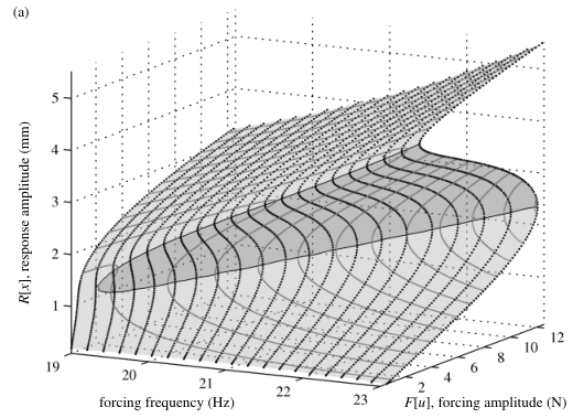

Figure 4 shows the time series recordings corresponding to the data points shown in Fig. 3(a); they demonstrate in detail the convergence of the method as the system passes through a saddle-node bifurcation (fold). The first harmonic of the input (Fig. 4(a)) gradually drifts during non-periodic transients but settles rapidly. The error (Fig. 4(b)) corresponds to the non-harmonic, invasive, part of the control; its decay during each step is evident. The vertical bars (marked , and ) indicate the stages of the iteration: step 2 occurs from to , and step 4 occurs from to . The input and output after are then accepted as points on the branch. Figure 4(c) shows the amplitude of the first harmonic of the displacement to further demonstrate convergence.
The main advantage of the method presented here over methods based on Newton iterations, apart from ease of implementation, is the speed-up of a factor of compared to [28, 21] (a conservative estimate; only individual solution curves could be traced out in [28, 21]). This feature is particularly important if one wants to explore systems that gradually degrade under laboratory conditions.
As illustrated in Fig. 5(a), this speed-up enables tracking of entire surfaces and the associated bifurcations. The experimental data points (marked by black dots in panels (a) and (b)) are obtained by consecutive runs for fixed frequencies Hz apart. The total experimental time to generate these results was 61 minutes. Panel (a) shows the three-dimensional projection in the space spanned by the two parameters forcing frequency and amplitude and the response amplitude (note that the response is non-harmonic and so this is indeed only a projection). Its main feature is the curve of saddle-node bifurcations passing through a cusp bifurcation (black). To facilitate the extraction of geometric information, the data points in Fig. 5 are interpolated using Wendland’s compactly supported radial basis functions [30, Ch. 11]. Using the interpolant, the bifurcation and constant forcing amplitude curves in Fig. 5(a,b) are calculated using numerical continuation on the experimentally generated surface. Curves of constant forcing amplitude (gray), reminiscent of the resonance curves for an idealized Duffing oscillator, give additional geometric information. All the data points within the dark gray shaded area of Fig. 5(a) are unstable periodic orbits of the uncontrolled system, and would typically not be seen experimentally.
Figure 5(b) shows a top-down view of panel (a), a two-parameter bifurcation diagram, again indicating all measured points on the unstable part of the surface in a darker shade of gray. The saddle-node bifurcation (fold) curve bounds the instability region with a cusp point at approximately Hz.
Figure 5(c) shows a front view of panel (a) with the error at each data point rendered onto the surface. Here the error is defined as the root-mean-square (RMS) of the non-harmonic part (defined in (17)) over one period. This is a measure of the invasiveness of the control; if this method was truly non-invasive, then this error would be zero. In the experimental set-up here the error is low, with a mean error of . The predominant source of error is noise amplification through the use of a derivative controller. This error is kept to a minimum through the use of the Butterworth filter described in section III. As seen in Fig. 5(c), there is no apparent correlation between geometric features of the solution surface (e.g., the fold points) and the magnitude of the error at that point.
V Conclusion
The presented approach is a general experimental technique to explore dynamical systems in parameter studies near saddle-node bifurcations (folds). It is particularly useful for the exploration of families of equilibria because no iterations similar to (9) are necessary. As we demonstrated, it is also applicable to periodically forced systems (the generalization to a non-harmonic forcing is straightforward). The main limitation of the method is that control fails at the linear level whenever the system does not depend on the bifurcation parameter to first order (e.g., near transcritical bifurcations). As the presented approach works particularly well around saddle-nodes, its main application areas are likely complementary to those of Pyragas’ TDF control. Examples currently under investigation include the identification of growth rates in chemostats [31, 32], or tracking localized spots in ferrofluids [33].
There are several ways in which this method can be generalized. First, if the equilibrium has more than a single unstable dimension, one typically reconstructs a proxy for the state through an observer [13] and lets depend on . This is a generalization of the use of PD control in the sections I.2 and III. Second, if one has more than a single adjustable system parameter then one can obtain multi-parameter families of equilibria and apply feedback control through more than a single input. Similarly, if one uses more than a single output (, ), one can feed back the input depending on the multi-dimensional , making control easier to achieve.
Acknowledgments: The research of J.S. is supported by EPSRC Grant EP/J010820/1.
References
- [1] E. H. Abed, H. O. Wang, and R. C. Chen, Physica D 70, 154 (1994).
- [2] K. Pyragas, Phys. Lett. A 170, 421 (1992).
- [3] J. E. S. Socolar, D. W. Sukow, and D. J. Gauthier, Phys. Rev. E 50, 3245 (1994).
- [4] K. Yamasue, K. Kobayashi, H. Yamada, K. Matsushige, and T. Hikihara, Physics Letters A 373, 3140 (2009).
- [5] A. Ahlborn and U. Parlitz, Phys. Rev. Lett. 93, 264101 (2004).
- [6] M. Kim, M. Bertram, M. Pollmann, A. v. Oertzen, A. S. Mikhailov, H. H. Rotermund, and G. Ertl, Science 292, 1357 (2001).
- [7] S. Schikora, H.-J. Wünsche, and F. Henneberger, Phys. Rev. E 83, 026203 (2011).
- [8] S. Schikora, P. Hövel, H.-J. Wünsche, E. Schöll, and F. Henneberger, Phys. Rev. Lett. 97, 213902 (2006).
- [9] O. Lüthje, S. Wolff, and G. Pfister, Phys. Rev. Lett. 86, 1745 (2001).
- [10] D. J. Christini, J. J. Collins, and P. S. Linsay, Phys. Rev. E 54, 4824 (1996).
- [11] C. von Loewenich, H. Benner, and W. Just, Phys. Rev. E 82, 036204 (2010).
- [12] E. Schöll and H. G. Schuster, eds., Handbook of Chaos Control, 2nd ed. (Wiley, New York, 2007).
- [13] E. D. Sontag, Mathematical Control Theory: Deterministic Finite Dimensional Systems (Springer, 1998).
- [14] B. Fiedler, V. Flunkert, P. Hövel, and E. Schöll, The European Physical Journal - Special Topics 191, 53 (2010).
- [15] V. Flunkert and E. Schöll, Phys. Rev. E 84, 016214 (2011).
- [16] B. Fiedler, V. Flunkert, M. Georgi, P. Hövel, and E. Schöll, Phys. Rev. Lett. 98, 114101 (2007).
- [17] H. Nakajima, Phys. Lett. A 327, 44 (2004).
- [18] E. W. Hooton and A. Amann, Phys. Rev. Lett. 109, 154101 (2012).
- [19] A. Tamasevicius, G. Mykolaitis, V. Pyragas, and K. Pyragas, Phys. Rev. E 76, 026203 (2007).
- [20] J. Sieber, A. Gonzalez-Buelga, S. A. Neild, D. J. Wagg, and B. Krauskopf, Phys. Rev. Lett. 100, 244101 (2008).
- [21] D. A. W. Barton, B. P. Mann, and S. G. Burrow, Journal of Vibration and Control 18, 509 (2012).
- [22] D. A. W. Barton and S. G. Burrow, ASME Journal of Computational and Nonlinear Dynamics 6, 011010 (2011).
- [23] E. Bureau, F. Schilder, I. Santos, J. Thomsen, and J. Starke, in Proceedings of ENOC 2011 (Rome, Italy, 2011).
- [24] E. Bureau, I. Santos, J. Thomsen, F. Schilder, and J. Starke, in Proceedings of the ASME 2012 IDETC (Chicago, IL, USA, 2012).
- [25] J. S. Anderson, S. Y. Shvartsman, G. Flätgen, I. G. Kevrekidis, R. Rico-Martinez, and K. Krischer, Phys. Rev. Lett. 82, 532 (1999).
- [26] P. Hövel and E. Schöll, Phys. Rev. E 72, 046203 (2005).
- [27] P. Hövel, Control of Complex Nonlinear Systems with Delay, Springer Theses (Springer, 2011).
- [28] J. Sieber and B. Krauskopf, Nonlinear Dynamics 51, 365 (2008).
- [29] A. Cammarano, Increasing the bandwidth of resonant vibration-based energy harvesters, Ph.D. thesis, University of Bristol (2012).
- [30] G. E. Fasshauer, Meshfree approximation methods with MATLAB (World Scientific, 2007).
- [31] A. J. Veraart, E. J. Faassen, V. Dakos, E. H. van Nes, M. Lurling, and M. Scheffer, Nature 481, 7381 (2012).
- [32] A. Rapaport, J. Sieber, S. Rodrigues, and M. Desroches, Bioprocess and Biosystems Engineering , online first (2013).
- [33] C. Gollwitzer, I. Rehberg, and R. Richter, New Journal of Physics 12, 093037 (2010).