Hot Gas, Cold Gas and Sub-Halos in a Lyman- Blob at Redshift 2.38
Abstract
We present integral field spectroscopy of a Lyman- blob at redshift 2.38, with a spectral resolution three times better than previous published work. As with previous observations, the blob has a chaotic velocity structure, much of which breaks up into multiple components. Our spectroscopy shows, however, that some of these multiple components are extremely narrow: they have velocity widths of less than .
Combining these new data with previous observations, we argue that this Lyman- blob resides in a dark-matter halo of around . At the centre of this halo are two compact red massive galaxies. They are surrounded by hot gas, probably a super-wind from merger-induced nuclear starbursts. This hot gas has shut down star formation in the non-nuclear region of these galaxies, leading to their red-and-dead colours.
A filament or lump of infalling cold gas is colliding with the hot gas phase and being shocked to high temperatures, while still around 30kpc from the red galaxies. The shock region is self-absorbed in Lyman- but produces C IV emission.
Further out still, the cold gas in a number of sub-halos is being lit up, most likely by a combination of tidally triggered star formation, bow-shocks as they plough through the hot halo medium, resonant scattering of Lyman- from the filament collision, and tidal stripping of gas which enhances the Lyman- escape fraction. The observed Lyman- emission from the Blob is dominated by the sum of the emission from these sub-halos.
On statistical grounds, we argue that Lyman- blobs are not greatly elongated in shape, and that most are not powered by ionisation or scattering from a central active galactic nucleus or starburst.
Keywords:
galaxies: haloes – galaxies: high-redshift.1 Introduction
Since their first discovery (Francis et al., 1996; Steidel et al., 2000), Lyman- blobs have held out the prospect of allowing us to study the spatially resolved flows of gas around massive young galaxies. While some Lyman- blobs surround high-redshift radio galaxies, and are clearly associated with AGN jets (Reuland et al., 2003; Reuland et al., 2007, e.g.), many are not. For these, a wide range of models have been proposed to explain their extended morphology and immense luminosities, including superwinds (Taniguchi et al., 2001, e.g.), infalling gas (Francis et al., 1996; Dijkstra et al., 2006, e.g.) and resonant scattering (Steidel et al., 2011, e.g.).
Integral field spectroscopy is an ideal way to map the velocity structure in these low-surface-brightness objects. Such spectroscopy has been published for four Lyman- blobs to date, and all show a similar pattern. LAB1 (Bower et al., 2004; Weijmans et al., 2010) shows no large-scale systematic velocity field, and multiple velocity components. Many, but not all of the Lyman- components seen here are seemingly associated with galaxies. Yang et al. (2011) observed blobs CDFS-LAB1 and CDFS-LAB2. They too find that the blobs break up into multiple velocity components, which seem to be associated with galaxies. They also find (for CDFS-LAB2) that the Lyman- emission is self-absorbed at the systemic redshift, with most emission coming at redder wavelengths. Wilman et al. (2005) observed LAB2 and saw absorption at one wavelength crossing their entire field, which they interpreted as absorption in a shell of gas swept up by a superwind, but an alternative interpretation is that it is due to a self-absorbing cloud of gas ionised from within, along the lines suggested by Zheng & Miralda-Escudé (2002). Otherwise LAB2 shows the same multiple emission components seen in LAB1.
Thus all four of the Lyman- blobs observed to date with spatially resolved spectroscopy show the same pattern: spatially extended but spectrally narrow emission components, often associated with stars, with no clear systematic velocity structure.
In this paper we present integral field spectroscopy of the first Lyman- blob found, (LAB1J2143−4423, hereafter B1), originally discovered by Francis et al. (1996). Our observations have a spectral resolution at the wavelength of Lyman- four times better than that of the previous observations, which turns out to be unexpectedly informative.
In an appendix, we also present spectroscopy of other Lyman- blob candidates in the same region of the sky.
Throughout this paper we adopt a cosmology with , and , based on the five year WMAP results (Hinshaw et al., 2009). Distances are proper unless otherwise specified.
2 Target
The Lyman- blob B1, originally discovered by Francis et al. (1996) has also been studied in Francis et al. (1997), Francis et al. (2001), Colbert et al. (2006) and Colbert et al. (2011). This blob remains one of the brightest and best-studied of the Lyman- blobs. In this section, existing observations of this blob, as reported in the above papers, are summarised.

Hubble Space Telescope (HST) imaging (Francis et al., 2001) shows that B1 consists of two compact red galaxies separated by (6 kpc), with a faint blue filament extending around 50 kpc to the south (Fig 1). The blue filament can be explained as a region of ongoing star formation, with little dust and a star-formation rate of around (Francis et al., 2001). The two compact red galaxies are more complicated. Francis et al. (2001) showed that their colours could be explained either by an old ( Myr) stellar population, or by a younger one obscured by dust.
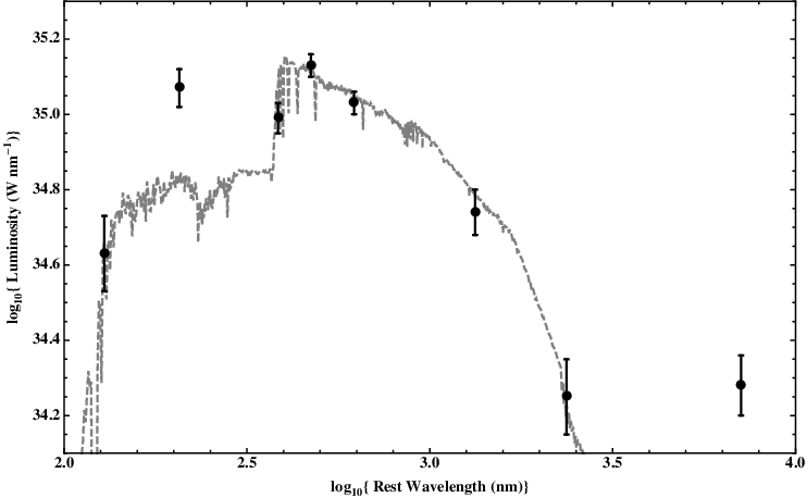
The mid-IR photometry presented by Colbert et al. (2011) allows this degeneracy to be resolved (Fig 2). We combined the optimally weighted photometry, summed over all the components, from Francis et al. (1996), Francis et al. (1997) and Francis et al. (2001) with the Spitzer photometry from Colbert et al. (2006) and Colbert et al. (2011), to get the spectral energy distribution shown in Fig 2. As the different components of B1 were not resolved in most of these data, the spectral energy distribution is an integrated one. These data were then compared to spectral synthesis models from Bruzual & Charlot (2003), combined with dust absorption following the empirical starburst extinction curve of Calzetti et al. (1994). The compact red galaxies can be fit by a simple instantaneous burst stellar population of age of 100-500 Myr, dust extinction with mag, and stellar mass of . They are thus massive but “red and dead”, with no substantive star formation for at least years. Additional blue emission from the filament explains the two shortest wavelength data points. B1 is a much more luminous source at 24 microns than this model predicts and shows poly-aromatic hydrocarbon (PAH) emission. This implies that a dusty starburst with a star formation rate of around is present, most likely in the core of one or both of the red galaxies (Colbert et al., 2006).
The Lyman- emission in B1 is genuinely diffuse. Intermediate band HST imaging shows that 13% of the Lyman- emission comes from the eastern red compact galaxy, but the rest is not coming from clumps smaller than a few kpc in size, as otherwise we would have seen the clumps.
Strong C IV (154.9 nm) emission is detected from B1 (Francis et al., 1996). Curiously, it is coming not from the location of the red galaxies, but from 25 kpc south along the filament, and occurs at a wavelength to the blue of most of the Lyman- emission (Fig 3).

B1 lies at redshift 2.38, in the middle of a supercluster (Francis & Hewett, 1993; Palunas et al., 2004) traced by QSO absorption lines and Lyman- emitting galaxies. Spectroscopy of three previously unclassified objects within this supercluster is reported in the Appendix A.
3 Observations and Reduction
B1 was observed on the night of August 1 2011, using the WiFeS integral field spectrograph (Dopita et al., 2007; Dopita et al., 2010) on the 2.3m telescope at Siding Spring Observatory. WiFeS uses an array of 25 slits, each 38 arcsec long and 1 arcsec wide to obtain integral field spectroscopy of a arcsec field. The total integration time on B1 was 4.5 hours. Seeing was around 1.3 arcsec. The B3000 grating was used, giving a spectral resolution of 100 km/s. The data presented here were reduced using a custom set of scripts written in Mathematica. After bias and overscan subtraction, and flat fielding, the individual slits were traced and straightened. Cosmic rays were identified by comparison with a median of the individual images. Very intense cosmic ray hits (probably the result of beta-decay in the substrate) were found to produce an exponential tail, presumably due to some charge transfer problem. This appeared to be a threshold effect, only occurring for the brightest cosmic rays, and having a constant amplitude and shape for them. These tails were thus easily identified and removed.
Wavelength calibration was done globally, to avoid introducing any row-to-row noise into the reconstructed data cube. Firstly, a polynomial wavelength dispersion relation was found for each spectral row in each slit. A fifth order polynomial was required to fit the arc lines in an individual row. Each of the derived polynomial coefficients was then plotted as a function of slit number and position within each slit. A linear or cubic fit to the variation in each polynomial coefficient was then derived. These fits were then used to reconstruct the wavelength solution for any part of the data. A root-mean-squared residual of 0.013nm was achieved across all arc-lines in all parts of the data, with no systematic patterns to the residuals. Sky lines in reconstructed data cubes were well aligned both along and across slits.
4 Results
The only line detected in the WiFeS data was the Lyman- line of blob B1. Different views of the data cube centred on B1’s Lyman- line are shown in Figs 4, 5, 6 and 3.


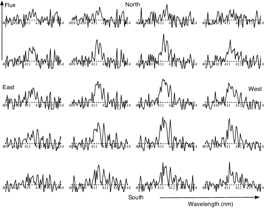
The velocity field is clearly a complex one. A number of conclusions can be drawn:
- 1.
The Lyman- emission from B1 is elongated by around 80 kpc in a north-south direction. The northern end corresponds to the red galaxies, and the southern end to the blue filament.
- 2.
- 3.
There is a gap in the emission at around 411.7 nm wavelength.
- 4.
The emission, particularly at the southern end, shows a complex velocity structure, with multiple emission and/or absorption components which are spectrally very narrow ().
- 5.
The C IV emission seen by Francis et al. (1996) comes from the southern end of B1, but at a wavelength blueward of nearly all the Lyman- emission.
Note that these observations are only picking up the higher surface-brightness parts of B1: our previous observations showed that low surface-brightness Lyman- emission extends far to the north-east of the region discussed here. We also know that a QSO sight-line passing around 160 kpc to the north-west intercepts a Lyman-limit absorption-line system (Francis & Williger, 2004), indicating that dense neutral hydrogen can be found far beyond the extent of the observable Lyman- emission.
This zig-zag velocity structure, interrupted by a gap, cannot easily be explained by a single rotational, infall or outflow model. It could be explained by a combination of separate components. Note that it is unlikely that the velocity structures we see are related one-to-one with gas structures. Due to the high optical depth in Lyman-alpha, the emission from any slab of gas structure is likely offset in velocity from its systemic velocity (Zheng & Miralda-Escudé, 2002; Schaerer et al., 2011, e.g.), and one slab of gas may produce two or more emission components, typically in the velocity wings. Nonetheless, radiative transfer effects typically broaden lines, so our upper limit on the velocity dispersions of around 100 is thus an upper limit on the velocity dispersion in the gas slabs from which this emission arises.
5 Discussion
Our observations show a very similar pattern to the previous integral field observations: no simple large-scale systematic velocity field, multiple sub-components, some associated with galaxies. However, our better velocity resolution, combined with the extensive multi-wavelength data-set available for this well studied blob, allows us to draw some somewhat more detailed conclusions than previous authors.
Our discussion starts with a puzzle, an hypothesis and a constraint.
5.1 Puzzle
The puzzle concerns gas in B1. The extensive Lyman- nebula implies the presence of large amounts of cool gas. In contrast, the red-and-dead colours of the compact red galaxies imply that there has been little star formation over a period lasting at least 100 Myr, and hence little cool gas. On the other hand, the mid-IR luminosity and PAH detection indicate prolific star formation and hence large quantities of molecular gas.
The resolution to this puzzle is to have different phases of gas on different scales. The starburst is most likely very compact ( kpc) and found in the nuclear regions of one or both of the compact red galaxies. It is so obscured by dust that no sign of it is seen at rest-frame wavelengths shorter than around (Fig 2). This nuclear starburst (or starbursts) is probably driven by the interaction between the two red galaxies, which lie at a projected separation of only 6 kpc. This picture is consistent with the expectations of the Kennicutt Jr. (1998b) star formation law in which the surface rate of star formation is related to the surface density of gas though . Regions of high specific star formation are therefore regions of high gas (and dust) surface densities, and are therefore likely to be heavily dust-obscured. The Lyman- emission we detect from one of the red galaxies would presumably be coming from the outskirts of the galaxy.
On scales of a few kpc, the gas is probably too hot to allow star formation. This explains the red-and-dead colours of the compact red galaxies. A superwind is likely present, as nuclear starbursts as luminous as that in B1 virtually always produce superwinds in the local universe (Veilleux et al., 2005, e.g.). This could have swept out any cool gas and truncated star formation in the outer regions of these galaxies. Taniguchi et al. (2001) suggested such superwinds as power-sources for Lyman- blobs. The age of the stellar population ( years) is comparable to the merger timescale, and the current star-formation rate, acting over years would produce a stellar mass comparable to that observed. The gas may also, however, have been heated by a concealed active galactic nucleus (King et al., 2011, e.g.) or by the liberation of potential energy from infalling gas (Johansson et al., 2009, e.g.).
We now turn to the neutral hydrogen responsible for the Lyman- nebula. This presumably lies further out, and is the subject of our hypothesis.
5.2 Hypothesis
Our data show that the extended Lyman- flux is typically tens of kpc from the red galaxies (which we assume lie at the centre of the dark matter halo), spatially extended on scales of several kpc, but breaks up spectrally into narrow sub-components. All these properties sound similar to those of a family of dwarf galaxies surrounding a massive galaxy. Which led us to the following hypothesis: that much of the extended Lyman- flux is coming from neutral gas within dark-matter sub-halos, moving within the much more massive dark matter halo centred on the red galaxies.
How feasible is this model? The relative velocities of the sub-clumps are , and they are spread over , which gives a virial mass of the main halo of . We selected ten such massive halos from the Millenium II n-body simulation (Boylan-Kolchin et al., 2009) at this redshift, and looked at the sub-halo population of these ten big halos. There were typically 10 – 20 sub-halos within each big halo. They were spread over around 100 kpc, and had a line-of-sight velocity dispersion of around . And the velocity dispersions of the individual sub-halos were typically around . Thus, the observational and the predicted parameters appear to match each other very well. These sub-halos in the simulation had typical dark matter masses of or more and half-mass radii of 1 – 5 kpc.
Would one expect sub-halos such as these to contain neutral hydrogen? We picked out a sample of small halos with masses of from the semi-analytic models of De Lucia & Blaizot (2007) applied to the Millenium I simulation (Springel et al., 2005), and they typically had cold gas masses of . So current semi-analytic models do suggest that at these redshifts, halos with masses of will contain reasonable amounts of neutral gas.
Why are these sub-halos radiating Lyman- emission? The sub-clumps we observe have Lyman- luminosities of , which are well within the range found in observed Lyman- emitting galaxies. However, the space density of halos is vastly greater than the space density of Lyman- emitting galaxies (Guaita et al., 2010, e.g.). Thus most such halos do not radiate at this level. The equivalent widths are also different: we compared the equivalent widths of blobs with those of compact Lyman- emitting galaxies in two surveys: Palunas et al. (2004) and Matsuda et al. (2004). Both surveys measured the equivalent widths (or equivalently narrow-band minus broad-band colour) for both the blobs and other Lyman- emitting galaxies in their fields, and in both cases, blobs were picked purely on the basis of size in the narrow-band image. In both cases, Lyman- blobs tend to have higher equivalent widths. A Kolmogorov-Smirnov two-sample test shows that the difference is significant at the 95% confidence level for the Palunas data, and at the 99.7% confidence level for the larger Matsuda dataset (using objects brighter than a narrow-band magnitude of 24.2). We therefore conclude that Lyman- blobs have significantly higher equivalent widths.
Thus for the hypothesis to be valid, we need some mechanism which increases the Lyman- luminosity and equivalent width of sub-halos when they are within the dense environment of massive halo, compared to the values seen in similar mass halos in less dense environments. We will discuss the possibilities in Section 5.4.
Note that some of these sub-halos may contain stars at this redshift. Sensitive observations may thus find that most, but probably not all of the Lyman- clumps have faint galaxies within them. Prescott et al. (2011a) recently presented imaging showing that one Lyman- blob does indeed seem to comprise a compact group of dwarf galaxies, though in this case the galaxies were not clearly associated with the Lyman- emission. Weijmans et al. (2010), however, did find that most clumps of Lyman- emission were centred on faint galaxies. So this is plausible.
5.3 The C IV Constraint
We now come to our constraint: the strong C IV (154.9 nm) emission detected coming from kpc south of the red galaxies. As discussed in Francis et al. (1996), C IV requires a hard ionising spectrum and must therefore either come from Active Galactic Nucleus (AGN) photoionisation or from fast shocks. We will discuss these possibilities in turn.
5.3.1 AGN Model
For the AGN model to work, we would require that at least one of the red galaxies hosts a type-2 AGN. Our line-of-sight to the AGN is blocked by a dusty torus, but UV radiation is escaping at least in the southerly direction, and impacting on some relatively dense gas cloud, where it produces Lyman- and C IV via photoionisation (Haiman & Rees, 2001; Adelberger et al., 2006; Francis & McDonnell, 2006, e.g.). A second mechanism, excitation by collision with a radio jet, is ruled out by our upper limit on the radio flux from B1 (Francis et al., 1996).
The first argument against this model is the detection of PAH emission from B1, which suggests that if a concealed AGN is present, its energy output is dominated by that from star formation. Note however that the PAH emission was only tentatively detected (Colbert et al., 2011), and that even an AGN which makes no significant contribution to the total energy output could still produce significant photoionisation.
A second argument against the AGN model is statistical. If the AGN model is correct, and the ratio of obscured to unobscured AGN is , then if we see blobs in a field, we should see unobscured AGN. We know that r is not significantly greater than 3 (Webster et al., 1995; Francis et al., 2004a; Treister et al., 2009, e.g.).
In the Palunas et al. field, we have three (or four if you count B5) Lyman- blobs. How many QSOs lie in this field at our redshift? Two QSOs were identified at the cluster redshift, one with at coordinates 21:42:31.33 -44:30:16.8 found by Francis et al. (2004a), and B29 identified by our GMOS observations described in Appendix A, with . In the field surveyed by Matsuda et al. (2004), there are 35 Lyman- blobs, and five known QSOs with optical magnitudes in the range 20.5 to 24.5, found in the NASA Extragalactic Database. In the survey by Yang et al. (2009), there are four Lyman- blobs and no QSOs down to the Sloan Digital Sky Survey limit of .
Combining these samples, we find that we can get suitable numbers of unobscured QSOs to be consistent with the blob population, but only if we include faint QSOs: those down to or fainter.
Could QSOs this faint feasibly enhance the Lyman- emission from nearby gas clouds to give the luminosity we observe in Lyman- blobs? We can answer this empirically by looking at the observed ratio of QSO magnitude to the flux of extended Lyman- emission around it. Weidinger et al. (2005) and Christensen et al. (2006) between them detected extended Lyman- emission around 9 QSOs. The average extended Lyman- flux was , which is comparable to Lyman- blob fluxes, so QSOs certainly can produce extended emission as seen in Blobs. However, the QSOs were very bright: averaging : much brighter than the QSOs found in the various Blob fields. And many QSOs this bright in the Weidinger and Christensen samples had no detectable extended Lyman- flux around them, so this average ratio of extended flux to nuclear flux is really only an upper limit. If we assume that the extended flux scales with the nuclear flux, then the QSOs in the blob fields are around two orders of magnitude less luminous than would be needed to produced the observed Lyman- blob flux. Would we expect the extended flux to be proportional to the photoionising luminosity? It is possible that the most luminous QSOs actually suppress the Lyman- emission of nearby galaxies, as suggested by Francis & Bland-Hawthorn (2004). In this case, less luminous QSOs might be surrounded by stronger Lyman- fuzz than the most luminous ones (which are the only ones studied to date), and hence might be plausible unobscured counterparts of Lyman- blobs. We note, however, that we did not detect extended Lyman- emission from either of the QSOs lying within our supercluster.
We therefore conclude that if blobs contain concealed QSOs, and these concealed QSOs are of comparable luminosity to the other QSOs seen in the blob fields, then they are unlikely to be luminous enough to produce the extended Lyman- emission through photoionisation. If the concealed QSOs are much more luminous, then it becomes difficult to understand why we don’t see at least a few comparably luminous unobscured QSOs in these fields, unless the radiation from these QSOs is completely blocked, in which case it cannot escape to photoionise the extended Lyman- emission. Thus while the AGN model cannot be ruled out for individual blobs, for statistical reasons it is unlikely that AGN photoionisation is the dominant power source of the population of Lyman- blobs.
5.3.2 Fast Shocks Model
Francis et al. (1996) and Francis et al. (2001) originally suggested that fast shocks could cause the C IV emission from B1, and demonstrated that they could produce ample line emission provided the density of the medium into which they were passing was at least and the shocks had become radiative, which required a timescale of years, which is comparable to the infall time for B1 and hence plausible.
Fast shocks are almost inevitable given the high velocity dispersion and observed lumpiness of the gas around B1. A plausible location for the shocks would be a collision between a superwind from the red galaxies and gas infalling along a filament from the south.
What is the infalling gas which is being shocked? One possibility is gas within an infalling sub-halo, perhaps an unusually massive one. Another is cold-mode infall (Faucher-Giguère et al., 2010; Goerdt et al., 2010, e.g.). The infalling gas cannot, however, be primordial, as we need it to contain carbon. The presence of a superwind is not necessary for this model to work: the impact of an infalling cold gas cloud on the hot central medium will suffice to drive suitable shocks.
5.4 Making the Sub-Halos Glow
Our model, based on the puzzle, hypothesis and constraint discussed above, is summarised in Fig 1. To make it work, however, we have to find some mechanism to make the gas in each sub-halo emit a Lyman- luminosity of . There are several plausible mechanisms and we will discuss them in turn.
5.4.1 Induced Star Formation
The ram pressure of their passage through the hot medium, or tidal interactions, could perhaps trigger star formation in these sub-halos, which would in turn generate the Lyman- emission. If we take the observed Lyman- luminosities, assume a typical unobscured ratio of Lyman-/H of , and apply the relation between H luminosity and star formation rate from Kennicutt Jr. (1998a), then we infer star formation rates in each sub-clump of around 2-3 solar masses per year, and hence multiplying by the number of sub-clumps, a total star formation rate of around 10–20 solar masses per year. This would just about be consistent with producing the observed UV emission from the blue filament (which gave an inferred star formation rate of around ). In practice, however, the optical depth in Lyman- is likely to be so high that ratios of Lyman-/H will be closer to , which would raise the inferred star formation rate to levels that are inconsistent with the faintness of the observed blue continuum flux. Another way to say this is that the equivalent width of the Lyman- emission is higher than that observed for other Lyman- emitting galaxies, as discussed in Section 5.2. Star formation is thus unlikely to produce all the Lyman- emission, though it could produce some of it.
5.4.2 Infall-powered emission
A typical sub-halo, according to semi-analytic models, will have a cold gas mass of , and an infall time of years. If we divide the gravitational potential energy of the gas in a sub-halo by the infall time, we get a power of , which is 500 times greater than the observed Lyman- luminosity. Thus if we can convert even 1% of the gravitational potential energy into radiation, we can explain the brightness of the sub-halos.
One mechanism for doing this (Dijkstra & Loeb, 2009, e.g.) is cooling radiation of thermally heated gas. Another is shock ionisation. If we assume that each sub-halo has a neutral gas surface area of several tens of square kpc, then a Lyman- luminosity density of a few is needed to reproduce the observed luminosities. If a shock-wave is driven into this surface as the sub-halo moves through the ambient gas, this shock will produce a diffuse Lyman- emission. The model shock grids of Allen et al. (2008) show that such a Lyman- luminosity density can be easily produced, provided pre-shock densities are and shock velocities are . Higher velocities or densities give much higher luminosities, allowing smaller gas surface areas, or more self-absorption.
Thus infall is a viable model for producing at least a substantial part of the observed Lyman- luminosity.
5.4.3 Scattered Lyman- from a central source
One possibility is that the emission we see from the sub-halos is actually produced elsewhere, and is just being resonantly scattered by the sub-halos. The emission could be coming from the same region that generates the C IV emission (according to our model, a region ionised by fast shocks where infalling gas hits a superwind), or escaping from the nuclear starbursts in the red galaxies. We do not see Lyman- emission directly from these regions, due to their high optical depths, but instead we see part of it scattered into the wings of the velocity distribution and off nearby gas clouds. This mechanism was invoked by Steidel et al. (2011) to explain the faint diffuse Ly halos seen in stacked images of high redshift galaxies, and can lead to polarised Lyman- emission (Dijkstra & Loeb, 2008, e.g.). Hayes et al. (2011) found that the Lyman- emission in LAB1 was indeed polarised, though Prescott et al. (2011b) did not detect such polarisation in much shallower observations of a different Lyman- blob.
How plausible is such a model in the case of B1? Steidel et al. (2011) found that the extended Lyman- flux typically exceeded the compact central line flux by a factor of , and in our case, the extended Lyman- flux exceeds the central Lyman- flux (from one of the red galaxies) by a factor of 7, which is comparable.
If scattered Lyman- emission originally came from the superwind/infalling gas collision, then the UV emission producing it came from fast shocks (as we know from our C IV detection) and would hence have a very hard spectrum. This means that we would expect very high equivalent widths and little detectable UV continuum, as observed.
If, on the other hand, the scattered Lyman- emission originally came from star formation, as proposed by Steidel et al. (2011), we might expect to see UV emission from this star formation. We can estimate how bright it should be by scaling from the results of Steidel et al. (2011). B1 has a Lyman- surface brightness in its central few arcsec which is times that of the halos seen by Steidel et al., so one would expect blue continuum emission magnitudes greater than the of the galaxies studied by Steidel - i.e. we should expect . In fact, B1 has . The red galaxies in B1 show no evidence in their optical colours of any ongoing star formation: we only see evidence for it in the mid-IR. A similar problem occurs in LAB1, where the probable central galaxy is also red (Chapman et al., 2004). In both B1 and LAB1 there is plenty of star formation taking place, which is seen in the mid-IR and sub-mm, but little or no detectable UV light.
To put this another way, the star formation rate inferred from the observed blue light in B1 (the blue filament) of is insufficient to produce the phenomenal observed Lyman- luminosity. We would need to tap into the much greater star formation rate which is concealed by dust, most likely in the red galaxies ().
The only way out of this would be to make the radiation from starbursts anisotropic. We would not see it from our orientation, but it would escape in other directions, analogous to unified models of AGN. If this was the case, we would sometimes expect to see blobs in which the central starburst was exposed. These would look like compact Lyman- emitters surrounded by relatively faint fuzz, rather than diffuse blobs, but should have Lyman- luminosities greater than that of blobs. There are two potential exposed starbursts in the Palunas et al. supercluster: B5 (Appendix A) and B40 (Francis et al., 2004b). Both have Lyman- luminosities and line widths comparable to the three blobs in this field. B5 has a compact nucleus surrounded by relatively faint fuzz, while B40 is spatially unresolved. But the extended flux of these objects is much fainter than that of the Lyman- blobs, so if viewed from some other orientation they might well be blobs, but much fainter ones. There are thus no possible counterparts of the most luminous blobs in this field.
Thus the scattering model is feasible, but only if we are scattering emission generated by fast shocks, rather than by star formation.
5.5 Tidal streams
Regardless of the mechanism or mechanisms producing the Lyman- emission from the sub-clumps, one would expect some tidal stripping of gas from them in this dense environment, perhaps producing Magellenic-stream style gas streams. This extended narrow gas morphology will increase the escape fraction of Lyman- and help enhance the observed brightness of these sub-halos regardless of the cause of the emission.
5.6 Intrinsic shape of the Sub-halo Swarm
If Lyman- blobs are collections of sub-halos, are these collections roughly spherical or are they elongated? There is some evidence for blobs lying in filamentary structures (Erb et al., 2011) but is this reflected in their shapes?
In this section, we develop a simple toy-model of elongated Lyman- blobs, taking into account a selection effect which biases samples towards finding end-on blobs. We compare this to data on the apparent shapes of Lyman- blobs from Matsuda et al. (2004), and show that blobs are not highly elongated on average.
Let us model Lyman- blobs as cigar-shaped ellipsoidal distributions of line-emitting clouds. To keep the model simple, we assume that the observed Lyman- surface brightness of a blob is proportional to the length of our line of sight through the ellipsoidal distribution. We further assume that the long axis of the blob is a factor longer than the minor axis, and that we are observing at an angle to the long axis. Simple geometry then tells us that the observed surface brightness b is given by:
| (1) |
Any narrow-band search for Lyman- blobs will have a surface brightness cut-off. Blobs that would normally lie below this cut-off will make it into the sample if viewed end-on, so any sample will be biased towards blobs seen at small values of . How big is this bias? To estimate this, we need to know how the space density of Lyman- blobs increases as the surface brightness decreases. To parameterise this, we plotted the cumulative number of blobs found by Matsuda et al. (2004) against their surface brightness, down to the rough completeness limit of this sample (Fig 7). We fit the cumulative space density in this survey with a straight-line model: the best fit is:
| (2) |
Thus if blobs seen end-on are a magnitude brighter than those seen side-on, the end-on ones will be over-represented in a sample by a factor of around 10.

We assume that the cumulative number density has a power-law dependence on limiting magnitude, with an index chosen to reproduce this factor of ten. For any given surface-brightness enhancement, we can then calculate how many more blobs we should see. We further assume that in the absence of any selection effects, blobs are randomly orientated in three dimensions, which means that the probability of seeing a blob from a given angle is proportional to . The observed distribution is then the product of the random orientation with the bias towards end-on blobs, which comes out as:
| (3) |

Thus even quite modest elongations will have a strong impact on the viewing angle at which Lyman- blobs are seen. We thus confirm that there can be a bias towards small viewing angles .
If we assume a power-law intrinsic distribution of elongations ( values), we can then do a monte-carlo calculation of the distribution of observed axial ratios projected onto the sky (the ratio of the observed long- to short-axis of the blob), and compare this with the observed distribution taken from Matsuda et al. (2004). The results are shown in Fig 9.

This figure shows that most of the Lyman- blobs observed by Matsuda were not greatly elongated. The best fit is where the number of blobs with a given intrinsic elongation () is proportional to . Models in which elongated blobs are more common over-predict the number of blobs with large observed elongations.
The Millenium II simulations analysed in section 5.2 are also not strongly elongated. Some of the massive galaxies lie at the intersection of multiple filaments, but because the sub-halos lie along more than one filament, the projected distribution is typically not greatly elongated.
We therefore conclude that Lyman- blobs are not in general strongly elongated (though clearly a few are). Observed samples are biased towards viewing elongated blobs down their long-axis, but this bias is not sufficient to explain the observed predominance of nearly circular blobs.
6 Conclusions
As our observations of Lyman- blobs become better, the blobs appear more complicated. There is already evidence for multiple energy sources in different blobs (Colbert et al., 2011, e.g.). This paper suggests that for one blob at least, the origin of the surrounding gas is also complicated, combining merger-driven dense molecular gas in the nuclei, hot gas perhaps from a superwind and infalling lumpy colder gas. Our observations are consistent with seeing a massive galaxy being assembled by minor mergers, as described by Kereš et al. (2005), Johansson et al. (2009) and Oser et al. (2011), though with a major merger taking place at the same time.
Cosmological hydrodynamical models which include some combination of winds and infall are rapidly increasing in sophistication (Zheng et al., 2010; Goerdt et al., 2010; Schaerer et al., 2011; Faucher-Giguère et al., 2010; Zheng et al., 2011, e.g.) but most fail to predict the narrowness of the velocity sub-structures we see. The exception are the models of Goerdt et al. (2010), but the relative narrowness of the emission they predict is likely an artefact of the lack of radiative transfer in their models.
We conclude that high spectral resolution observations are providing an interesting challenge to the models. Few instruments are set up to make these high resolution observations in the blue, but those that can should pursue this.
Acknowledgments
We’d like to thank Ralph Sutherland for several useful conversations.
The Millennium Simulation databases used in this paper and the web application providing online access to them were constructed as part of the activities of the German Astrophysical Virtual Observatory.
Based in part on observations obtained as part of program GS-2005B-Q-23 at the Gemini Observatory, which is operated by the Association of Universities for Research in Astronomy, Inc., under a cooperative agreement with the NSF on behalf of the Gemini partnership: the National Science Foundation (United States), the Science and Technology Facilities Council (United Kingdom), the National Research Council (Canada), CONICYT (Chile), the Australian Research Council (Australia), Ministério da Ciîncia, Tecnologia e Inovação (Brazil) band Ministerio de Ciencia, Tecnología e Innovación Productiva (Argentina).
Based in part on observations made with the NASA/ESA Hubble Space Telescope, and obtained from the Hubble Legacy Archive, which is a collaboration between the Space Telescope Science Institute (STScI/NASA), the Space Telescope European Coordinating Facility (ST-ECF/ESA) and the Canadian Astronomy Data Centre (CADC/NRC/CSA).
Dopita acknowledges ARC support under Discovery project DP0984657.
Appendix A Slit mask spectroscopy of other candidate blobs in the Field
In this appendix, spectroscopy is presented of three other candidate Lyman- emitters which lie in the same supercluster as B1. All lie several arcminutes from B1 and so do not directly impact on its physics. Their properties are, however, used in the various statistical arguments in the main body of the paper.
We had previously obtained spectra of most bright potential Lyman- emitters in the supercluster surrounding B1 (Francis et al., 2004b), but three needed further observations. In this section we present spectroscopy of these three.
One, B5 in the list of Palunas et al. (2004) was classified as a potential Lyman- blob, albeit an unusual one. It consisted of a luminous narrow-band emitting core surrounded by faint narrow-band excess fuzz. Our previous spectrum of this object was ambiguous (Francis et al., 2004b): we saw a potential Lyman- line but also two other possible weak lines which did not match. The second object, identified by Palunas et al. (2004) and called B29 was the most luminous compact potential Lyman- emitter in the field, but had not been previously observed due to fibre collision constraints with the spectrograph. It is located at 21:43:05.90 44:27:21.0 (J2000). The third, B30, was a fainter narrow-band excess object found by Palunas et al, also not observed previously due to fibre placement issues. It is located at 21:43:06.42 44:27:00.6 (J2000).
B5, B29 and B30 were observed with the GMOS spectrograph on the Gemini South Telescope. The observational set-up with GMOS is described by Scarlata et al. (2009): both objects were observed simultaneously for an exposure time of 8,800 seconds, in 0.6 arcsecond seeing, on the night of 2005 October 9th.
From B5, we detect a single very strong emission line at 410.0 nm, with a velocity width of . The tentative additional lines seen by Francis et al. (2004b) were ruled out. On the basis of the line width, extended emission and equivalent width, so the line must be Lyman-. The Lyman- emission was slightly extended along the slit, so we confirm that B5 is an extremely luminous extended Lyman- emitting object at .
B29 turned out to be a QSO at the supercluster redshift. It showed strong broad Lyman- peaking at around 412.0 nm, as well as a number of other typical QSO broad lines. The line widths were around 440 nm (full width at half maximum height). Strong associated absorption was seen in Lyman- and C IV (154.9 nm), slightly red-shifted with respect to the emission-line peak.
B30 showed a single strong emission line at 412.2 nm, with a velocity width of , and is hence confirmed as a Lyman- emitting galaxy in the supercluster.
References
- Adelberger et al. (2006) Adelberger K. L., Steidel C. C., Kollmeier J. A., Reddy N. A., 2006, The Astrophysical Journal, 637, 74
- Allen et al. (2008) Allen M. G., Groves B. A., Dopita M. A., Sutherland R. S., Kewley L. J., 2008, Monthly Notices of the Royal Astronomical Society, 178, 20
- Bower et al. (2004) Bower R. G. et al., 2004, Monthly Notices of the Royal Astronomical Society, 351, 63
- Boylan-Kolchin et al. (2009) Boylan-Kolchin M., Springel V., White S. D. M., Jenkins A., Lemson G., 2009, Monthly Notices of the Royal Astronomical Society, 398, 1150
- Bruzual & Charlot (2003) Bruzual G., Charlot S., 2003, Monthly Notices of the Royal Astronomical Society, 344, 1000
- Calzetti et al. (1994) Calzetti D., Kinney A. L., Storchi-Bergmann T., 1994, The Astrophysical Journal, 429, 582
- Chapman et al. (2004) Chapman S. C., Scott D., Windhorst R. A., Frayer D. T., Borys C., Lewis G. F., Ivison R. J., 2004, The Astrophysical Journal, 606, 85
- Christensen et al. (2006) Christensen L., Jahnke K., Wisotzki L., Sánchez S. F., 2006, Astronomy and Astrophysics, 459, 717
- Colbert et al. (2011) Colbert J., Scarlata C., Teplitz H., Francis P., Palunas P., Williger G., Woodgate B., 2011, The Astrophysical Journal, 728, 59
- Colbert et al. (2006) Colbert J. W., Teplitz H., Francis P., Palunas P., Williger G. M., Woodgate B., 2006, The Astrophysical Journal, 637, L89
- De Lucia & Blaizot (2007) De Lucia G., Blaizot J., 2007, Monthly Notices of the Royal Astronomical Society, 375, 2
- Dijkstra et al. (2006) Dijkstra M., Haiman Z., Spaans M., 2006, The Astrophysical Journal, 649, 14
- Dijkstra & Loeb (2008) Dijkstra M., Loeb A., 2008, Monthly Notices of the Royal Astronomical Society, 386, 492
- Dijkstra & Loeb (2009) Dijkstra M., Loeb A., 2009, Monthly Notices of the Royal Astronomical Society, 400, 1109
- Dopita et al. (2007) Dopita M., Hart J., McGregor P., Oates P., Bloxham G., Jones D., 2007, Astrophysics and Space Science, 310, 255
- Dopita et al. (2010) Dopita M. et al., 2010, Astrophysics and Space Science, 327, 245
- Erb et al. (2011) Erb D. K., Bogosavljević M., Steidel C. C., 2011, The Astrophysical Journal Letters, 740, L31
- Faucher-Giguère et al. (2010) Faucher-Giguère C.-A., Kereš D., Dijkstra M., Hernquist L., Zaldarriaga M., 2010, The Astrophysical Journal, 725, 633
- Francis & Bland-Hawthorn (2004) Francis P. J., Bland-Hawthorn J., 2004, Monthly Notices of the Royal Astronomical Society, 353, 301
- Francis & Hewett (1993) Francis P. J., Hewett P. C., 1993, Astronomical Journal (ISSN 0004-6256), 105, 1633
- Francis & McDonnell (2006) Francis P. J., McDonnell S., 2006, Monthly Notices of the Royal Astronomical Society, 370, 1372
- Francis et al. (2004a) Francis P. J., Nelson B. O., Cutri R. M., 2004a, The Astronomical Journal, 127, 646
- Francis et al. (2004b) Francis P. J., Palunas P., Teplitz H. I., Williger G. M., Woodgate B. E., 2004b, The Astrophysical Journal, 614, 75
- Francis & Williger (2004) Francis P. J., Williger G. M., 2004, The Astrophysical Journal, 602, L77
- Francis et al. (2001) Francis P. J. et al., 2001, The Astrophysical Journal, 554, 1001
- Francis et al. (1997) Francis P. J., Woodgate B. E., Danks A. C., 1997, The Astrophysical Journal, 482, L25
- Francis et al. (1996) Francis P. J. et al., 1996, Astrophysical Journal v.457, 457, 490
- Goerdt et al. (2010) Goerdt T., Dekel A., Sternberg A., Ceverino D., Teyssier R., Primack J. R., 2010, Monthly Notices of the Royal Astronomical Society, 407, 613
- Guaita et al. (2010) Guaita L. et al., 2010, The Astrophysical Journal, 714, 255
- Haiman & Rees (2001) Haiman Z., Rees M. J., 2001, The Astrophysical Journal, 556, 87
- Hayes et al. (2011) Hayes M., Scarlata C., Siana B., 2011, Nature, 476, 304
- Hinshaw et al. (2009) Hinshaw G. et al., 2009, Monthly Notices of the Royal Astronomical Society, 180, 225
- Johansson et al. (2009) Johansson P. H., Naab T., Ostriker J. P., 2009, The Astrophysical Journal, 697, L38
- Kennicutt Jr. (1998a) Kennicutt Jr. R. C., 1998a, Annual Review of Astronomy and Astrophysics, 36, 189
- Kennicutt Jr. (1998b) Kennicutt Jr. R. C., 1998b, The Astrophysical Journal, 498, 541
- Kereš et al. (2005) Kereš D., Katz N., Weinberg D. H., Davé R., 2005, Monthly Notices of the Royal Astronomical Society, 363, 2
- King et al. (2011) King A. R., Zubovas K., Power C., 2011, Monthly Notices of the Royal Astronomical Society: Letters, 415, L6
- Matsuda et al. (2004) Matsuda Y. et al., 2004, The Astronomical Journal, 128, 569
- Oser et al. (2011) Oser L., Naab T., Ostriker J. P., Johansson P. H., 2011, The Astrophysical Journal, 744, 63
- Palunas et al. (2004) Palunas P., Teplitz H. I., Francis P. J., Williger G. M., Woodgate B. E., 2004, The Astrophysical Journal, 602, 545
- Prescott et al. (2011a) Prescott M. K. M. et al., 2011a, eprint arXiv:1111.0630
- Prescott et al. (2011b) Prescott M. K. M., Smith P. S., Schmidt G. D., Dey A., 2011b, The Astrophysical Journal Letters, 730, L25
- Reuland et al. (2007) Reuland M. et al., 2007, The Astronomical Journal, 133, 2607
- Reuland et al. (2003) Reuland M. et al., 2003, The Astrophysical Journal, 592, 755
- Scarlata et al. (2009) Scarlata C. et al., 2009, The Astrophysical Journal, 706, 1241
- Schaerer et al. (2011) Schaerer D., Hayes M., Verhamme A., Teyssier R., 2011, Astronomy and Astrophysics, 531, 12
- Springel et al. (2005) Springel V. et al., 2005, Nature, 435, 629
- Steidel et al. (2000) Steidel C. C., Adelberger K. L., Shapley A. E., Pettini M., Dickinson M., Giavalisco M., 2000, The Astrophysical Journal, 532, 170
- Steidel et al. (2011) Steidel C. C., Bogosavljević M., Shapley A. E., Kollmeier J. A., Reddy N. A., Erb D. K., Pettini M., 2011, The Astrophysical Journal, 736, 160
- Taniguchi et al. (2001) Taniguchi Y., Shioya Y., Kakazu Y., 2001, The Astrophysical Journal, 562, L15
- Treister et al. (2009) Treister E., Urry C. M., Virani S., 2009, The Astrophysical Journal, 696, 110
- Veilleux et al. (2005) Veilleux S., Cecil G., Bland-Hawthorn J., 2005, Annual Review of Astronomy and Astrophysics, 43, 769
- Webster et al. (1995) Webster R. L., Francis P. J., Petersont B. A., Drinkwater M. J., Masci F. J., 1995, Nature, 375, 469
- Weidinger et al. (2005) Weidinger M., Møller P., Fynbo J. P. U., Thomsen B., 2005, Astronomy and Astrophysics, 436, 825
- Weijmans et al. (2010) Weijmans A.-M., Bower R. G., Geach J. E., Swinbank A. M., Wilman R. J., de Zeeuw P. T., Morris S. L., 2010, Monthly Notices of the Royal Astronomical Society, 402, 2245
- Wilman et al. (2005) Wilman R. J., Gerssen J., Bower R. G., Morris S. L., Bacon R., de Zeeuw P. T., Davies R. L., 2005, Nature, 436, 227
- Yang et al. (2011) Yang Y., Zabludoff A., Jahnke K., Eisenstein D., Davé R., Shectman S. A., Kelson D. D., 2011, The Astrophysical Journal, 735, 87
- Yang et al. (2009) Yang Y., Zabludoff A., Tremonti C., Eisenstein D., Davé R., 2009, The Astrophysical Journal, 693, 1579
- Zheng et al. (2010) Zheng Z., Cen R., Trac H., Miralda-Escudé J., 2010, The Astrophysical Journal, 716, 574
- Zheng et al. (2011) Zheng Z., Cen R., Weinberg D., Trac H., Miralda-Escudé J., 2011, The Astrophysical Journal, 739, 62
- Zheng & Miralda-Escudé (2002) Zheng Z., Miralda-Escudé J., 2002, The Astrophysical Journal, 578, 33