Mechanisms for Fair Allocation Problems:
No-Punishment Payment Rules in Fully Verifiable Settings
Abstract
Mechanism design is addressed in the context of fair allocations of indivisible goods with monetary compensation. Motivated by a real-world social choice problem, mechanisms with verification are considered in a setting where (i) agents’ declarations on allocated goods can be fully verified before payments are performed, and where (ii) verification is not used to punish agents whose declarations resulted in incorrect ones. Within this setting, a mechanism is designed that is shown to be truthful, efficient, and budget-balanced, and where agents’ utilities are fairly determined by the Shapley value of suitable coalitional games. The proposed mechanism is however shown to be #P-complete. Thus, to deal with applications with many agents involved, two polynomial-time randomized variants are also proposed: one that is still truthful and efficient, and which is approximately budget-balanced with high probability, and another one that is truthful in expectation, while still budget-balanced and efficient.
1 Introduction
Whenever the outcome of some social choice process depends on the information collected from a number of self-interested agents, strategic issues may come into play. Indeed, agents may find convenient to misreport their types, i.e., the relevant information they own as their private knowledge, so that the best possible solution cannot be achieved. In these cases, mechanism design techniques can be used as solution approaches, which augment combinatorial algorithms with appropriate monetary payments, aimed at motivating all agents to truthfully report their private types (see, e.g., ?, ?).
On the class of social choice utilitarian problems, agent types encode (monetary) valuations over the set of all possible solutions and the goal is to compute a solution maximizing the social welfare, i.e., the sum of agents’ true evaluations. A prominent role in mechanism design for problems of this class is played by the Vickrey-Clarke-Grove (VCG) paradigm (?, ?, ?), which is a general method for designing truthful mechanisms, i.e., mechanisms where truth-telling is a dominant strategy for each agent. In particular, VCG mechanisms are efficient. That is, they guarantee that a solution maximizing the social welfare is actually computed. However, they are not budget-balanced, i.e., the algebraic sum of the monetary transfers is not zero and mechanisms from this class can run into deficit. In fact, this is a well-known drawback of VCG mechanisms (see, e.g., ?), but it is essentially the best one can hope to do, given classical impossibility theorems (?, ?), stating that no truthful mechanism can be designed to be always efficient and budget-balanced.
In many practical applications, as the one that inspired the present work, payments to agents can be performed after the final outcome is known, so that some kind of verification on reported types might be possible. Mechanisms with verification have been introduced by ? (?) and subsequently studied in a number of papers. For instance, ? (?) considered verification for a task scheduling problem: We have some agents declaring the amount of time they need to solve each task, and the goal is to have all tasks being solved, by minimizing the completion time of the last-solved one (hence, the make-span). In this context, payments are computed after the actual tasks release times have been observed, so that we have, for instance, the ability to “punish” some agent whose declared ability has been verified to be different than its actual performance in the process.
Note that the knowledge of the actual outcome represents a source of additional information to define payment rules, as it might partially reveal agents’ types. However, this additional power is not considered in the classical mechanism-design setting. In fact, whenever verification is allowed, some (classical) impossibility results might no longer hold.
Compared to standard mechanisms (see, e.g., ?), those with verification have received considerably less attention in the literature (see, e.g., ?, ?, ?, ?, ?). In particular, these works consider a verification ability that is partial, in the sense that agents’ (mis)reporting is restricted to true types plus certain lies (e.g., values that are lower than the true ones), and that verification is focused to detect such lies only. An extension of this basic model has been recently proposed by ? (?), who assume no a-priori restrictions on the agents’ reported types, within a setting where an agent cheating on her/his type will be caught with some probability that may depend on her/his true type, the reported type, or both. In fact, despite these different facets of the verification power, most of the mechanisms with verification proposed in the literature share the idea of providing incentives to truthfully report private types by exploiting the intimidation of punishing those agents that will be caught lying. Moreover, while budget limits have been considered in some approaches (see, e.g., ?), no mechanism with verification has been designed to be budget-balanced, with the focus being on truthfulness and efficiency.
In the paper, we study mechanisms with verification from the same perspective as ? (?), in particular by considering a setting where there is no restriction on the agents’ reported types. However, differently from this work, we assume that verification is deterministic, i.e., all incorrect declarations on allocated goods will be eventually detected. This leads to a stronger verification ability, which could be in principle used to easily enforce truthfulness by just punishing those agents whose declarations have been checked to be incorrect ones. However, such an approach would be hardly acceptable by agents in real-life applications, because a true punishment would require a clear proof of a malevolent behavior. Indeed note that, in practice, possible discrepancies between agents’ declarations and third-party verified values may be due to many different reasons, in particular to the subjective judgment of the verifier. Based on this observation and motivated by a real-world application domain, we will assume in the paper that only a limited use of such verification power can be made, and indeed that mechanisms have to be designed which are not based on punishments—while nonetheless resulting to be truthful, efficient, and even budget-balanced.
1.1 Mechanisms for Fair Division with Monetary Compensation
We consider mechanisms with verification in the context of fair allocation problems (see, e.g., ?, ?, ?). We assume that a set of indivisible goods to be allocated to a set of agents is given. Each agent is equipped with a private preference relation, which is just encoded as a real-valued function (basically, a monetary valuation) over all possible goods—formal definitions are in Section 3. An agent can have allocated more then one good, in which case her/his evaluation is additive over them. Moreover, goods are non-sharable, i.e., each good can be allocated to one agent at most. However, monetary transfers are allowed, in terms of both payments charged to agents and monetary compensations provided to them. The goal is to find an efficient allocation, that is, an allocation maximizing the total value of the allocated goods, by designing rules guaranteeing that certain desirable properties are achieved, such as truthfulness and individual rationality, i.e., no agent is ever worse off than he would be without participating to the mechanism. Moreover, we want to obtain outcomes that are “politically” acceptable. That is, agents should perceive the designed mechanism as a fair one (see, e.g., ?), independently of the rules leading them to be honest. For instance, it is desirable that no agent envies the allocation of any another agent, or that the selected outcome is Pareto efficient, i.e., there must be no different allocation such that every agent gets at least the same utility and one of them even improves.
Note that the above model for fair allocation is general enough to deal with many practical scenarios, and it has been indeed intensively studied in the literature. One example application is parking space and benefit allocation at a workplace, where each employee gets a parking space and a share from a fixed benefits package. House allocation problems are another classical example, where agents collectively own a set of houses, and we look for a systematic way of exclusively assigning a house to each agent, possibly with monetary compensations. A third example is job allocation among a group of employees, e.g., assigning an unexpected task among the business units of a corporate, where a job and possibly a monetary compensation is assigned to each employee. Finally, yet another classical application is room assignment-rent division, where a group of agents shall rent a house, with each of them getting a room and paying a share of the rent of the house.
The model and, in particular, properties of fair allocations with indivisible objects and monetary transfers have been studied, e.g., by ? (?, ?, ?, ?, ?, ?, ?, ?, ?, ?, ?, ?). Moreover, procedures to compute fair allocations have been proposed by ? (?, ?, ?, ?, ?, ?).
None of the above listed approaches, however, can guarantee the elicitation of honest preferences from the agents. In fact, the question of designing truthful and fair mechanisms has been recently considered as well (?, ?, ?, ?, ?, ?, ?). In these approaches, while budget limits are sometimes enforced and mechanisms are defined that cannot run into deficit, budget-balance is never guaranteed. Indeed, this comes again with no surprise, given that no truthful mechanism can be simultaneously fair (e.g., envy-free or Pareto-efficient) and budget-balanced (see, e.g., ?, ?, ?).
To circumvent this impossibility, approaches have been studied that focus on weaker notions of truthfulness. For instance, ? (?) and ? (?) consider a notion of degree of manipulability which can be used to compare the ease of manipulation in allocation mechanisms, whereas the notion of weak strategy-proofness is considered by ? (?), i.e., cheating agents are always risking an actual loss, and are never guaranteed to cheat successfully.
In this paper, we depart from the settings studied in all such earlier approaches, because we are interested in applications where a form of verification is available to the mechanism at the time of deciding monetary compensations among agents. It follows that the mechanism may exploit the knowledge of private agents’ types, and hence classical impossibility results may no longer hold. Indeed, by exploiting this knowledge, and even assuming a setting where agents with verified incorrect declarations are not punished, we can show that it is possible to design mechanisms for allocation problems that are truthful, efficient, budget-balanced, individually rational, and fair. Note that having this kind of a-posteriori knowledge at payment time is quite common to many applications. In fact, we were inspired by the following real-world scenario, which will be later formalized in Section 2.
1.2 The Italian Research Assessment Program (VQR) 2004-2010
In 2012, the National Agency for the Evaluation of Universities and Research Institutes (ANVUR) has promoted the ‘VQR’ assessment program devoted to evaluate the quality of the whole Italian research production in the period 2004-2010. Every research structure has to select some research products, and submit them to ANVUR. While doing so, the structure is in competition with all other Italian research structures, as the outcome of the evaluation will be used to proportionally transfer the funds that have been allocated by the Ministry to support research activities in the next years (until data from a new evaluation for the subsequent period will be available).
Every structure is then interested in selecting and submitting its best research products. To this end, the program is articulated in three phases. First, authors are asked to self-evaluate their products, according to some evaluation criteria defined by groups of experts chosen by ANVUR. Here, it is assumed that, having such criteria, every author is able to perform a ranking of her/his own products, ideally to equip each of them with a quality score.11 1 The set of the possible scores is defined in the VQR guidelines. To our ends, this detail is immaterial and scores are just viewed as (arbitrary) real numbers. In the second phase, based on the self-evaluations being collected, every structure selects and submits to ANVUR (at most) three products for each author affiliated to ,22 2 Actually, the number of publications is not always three, in some specific exceptions. Again, this is not a relevant issue, as we shall see in the formalization in Section 3. in such a way that the sum of the declared, i.e., self-assessed, scores of the selected products is the maximum possible one for structure , and that each product is formally associated to one author at most. Finally, ANVUR formulates its independent quality judgment about submitted publications, and the sum of their “true” scores (i.e., those resulting by ANVUR evaluation) is then the VQR score of . Eventually, will receive funds in the next years proportionally to this score.
In fact, a VQR score is assigned not only to the structure , but also to all its substructures (e.g., to Departments, if is a University). Of course, this has an impact on the funds redistribution inside every research structure. Therefore, while it is clear that each structure has to maximize the total value of the products submitted to ANVUR, whenever the same product has different co-authors, some strategic issues come into play and co-authors’ personal interest may induce them to cheat on the quality of their products, and may lead to choices going far from the optimum (total) value. We thus believe that mechanism design is of high practical interest in contexts resembling this one. In the mechanism, since products are indivisible, i.e., each of them can be formally allocated to one author at most, payments should reflect “adjustments” over the VQR scores, which suitably take into account the various co-authors no matter to whom any publication is actually allocated. Moreover, as payments can be computed at the end of the process on the basis of the VQR scores made available by ANVUR, a mechanism with verification can be conceived, with ANVUR playing the role of the verifier.
1.3 Contributions
Motivated by the above application scenario, in this paper, we study allocation problems in a strategic setting where agents can misreport their private types, and we study mechanisms with verification from both the algorithmic and the computational complexity viewpoint.
Algorithmic Issues. We show that in the given setting none of the classical impossibility theorems discussed above holds. In particular, we exhibit a payment rule that turns any optimal allocation algorithm, i.e., any algorithm computing an optimal allocation given the reported types, into a mechanism with verification such that:
-
The mechanism is truthful. This is shown by pointing out a number of properties of allocation problems which are of interest on their own.
-
The mechanism is efficient, budget-balanced, individually rational, envy-free, and Pareto efficient.
-
The mechanism satisfies the following properties, which are in fact crucial—and hence specifically discussed—for the case study of the Italian Research Assessment Program:
- –
The payment rule is indifferent w.r.t. the scores (possibly cheats) declared for goods that do not occur in the allocation being selected (and hence that are not verified). In theory, the feature is irrelevant given that truth-telling is a dominant strategy. In practice, this might be rather useful in the VQR program, because unsubmitted research products with their unverified declared scores should have no influence on the payments, as they have no influence on the actual score of the research structure after the evaluation is carried out. Moreover, it is unlikely that a consensus can be achieved on a mechanism where payments are based on unverified self-declarations.
- –
Verification is not used to force truthfulness by just punishing those agents whose reported values are found different from the verified ones. Again, the rationale is that a punishment approach would be hardly “politically” acceptable in this context (charging university professors because of their self-evaluation about some paper would require some convincing proof of their malicious behavior, and would start never-ending disputes).
- –
The payment rule is indifferent w.r.t. the specific optimal allocation being selected by the mechanism. Thus, the score of each researcher/substructure is univocally determined by the overall score of the structure, and any researcher/substructure does not have any reasonable argument against her/his structure because of possible alternative allocations. In fact, this is a very strong kind of fairness property, which immediately entails envy-freeness and Pareto-efficiency.
- –
-
Agents’ utilities are distributed according to the Shapley value of two suitably-associated coalitional games—see, e.g., (?), for a comprehensive introduction to sharing problems and coalitional games. In fact, the Shapley value is a prototypical solution concept for fair division with monetary compensations, and its desirable properties in (games associated with) allocation problems have been largely studied in the literature (e.g., ?, ?, ?).
Note that the Shapely value has been studied in mechanism-design contexts too, where emphasis has been given to the pricing problem for a service provider (?, ?, ?): The cost of providing a service is a function of the sets of customers, and the goal is that of determining which customers (and at a what price) have to receive it. The model gives rise to a cross-monotonic cost-sharing game, where Shapley-value based sharing mechanisms can be defined that are truthful and budget-balanced, and which achieve the lowest worst-case loss of efficiency over all utility profiles (?). With this respect, the pricing rule can abstractly be viewed as a witness that, whenever (partial) verification is possible, Shapley-valued based mechanisms may also be implemented with no loss of efficiency at all.
Complexity Issues. Computing an optimal allocation on the basis of the reported types is an easy task, which can be carried out via adaptations of classical matching algorithms. However, one might suspect that our mechanism is not computationally-efficient as it is based on the computation of a Shapley value. This is indeed a challenging task that involves iterating over all possible subsets of agents. We analyze these issues, and we provide the following contributions:
-
We show that computing the Shapley value for allocation problems is inherently intractable, in fact, #P-complete. Note that, while membership results for #P are rather common for problems involving Shapley value computations, #P-hardness results have only been proven so far for a few kinds of coalitional games, in particular, for weighted voting games (?) and minimum spanning-tree games (?).
-
In order to deal with scenarios with many agents demanding for computational efficiency, two modified rules, and , are presented, which are founded on a fully polynomial-time randomized approximation scheme for the Shapley value computation. The resulting polynomial-time mechanisms retain most of the properties of . In particular, the mechanism based on is truthful, efficient, and with high-probability it is approximately budget-balanced. Instead, the mechanism based on is truthful in expectation, but always efficient and budget-balanced.
Organization. The rest of the paper is organized as follows. The motivation scenario for the research reported in the paper is analyzed in Section 2. Then, Section 3 illustrates the formal framework and the basic concepts to design mechanisms with verification. The payment rule is defined and analyzed in Section 4. Connections with coalitional games are pointed out in Section 5, while rules and are defined in Section 6, where computational issues are dealt with. A comparison with some related works is reported in Section 7, while a few final remarks are eventually discussed in Section 8.
2 Motivating Example: The Italian Research Assessment Program (VQR) 2004–2010
In this section we describe the motivating example and case study of the present work: the program for evaluating all Italian research structures for their activities in years 2004–2010. The evaluation is performed by ANVUR, the National Agency for the Evaluation of Universities and Research Institutes (www.anvur.org). Substructures (e.g., University departments) will also be evaluated, by considering the researchers affiliated to them.
2.1 Formalization
Let us hereinafter focus on a given structure , let be the set of researchers affiliated to and, for each , let be the set of the research products of in the given period 2004-2010. In the first phase of the program, each researcher associates a quality score with each product .
An allocation for is then a function mapping each researcher to a set of publications with and with , for each . In the second phase, the structure computes an optimal allocation, i.e., an allocation such that , for each possible allocation . The goal of structure is indeed to maximize its total score (social welfare), and thus the funds that eventually will receive. Note that this optimization phase is based on the scores declared by researchers. Therefore, the goal of will be achieved if authors correctly/truthfully self-evaluate their products.
Example 2.1.
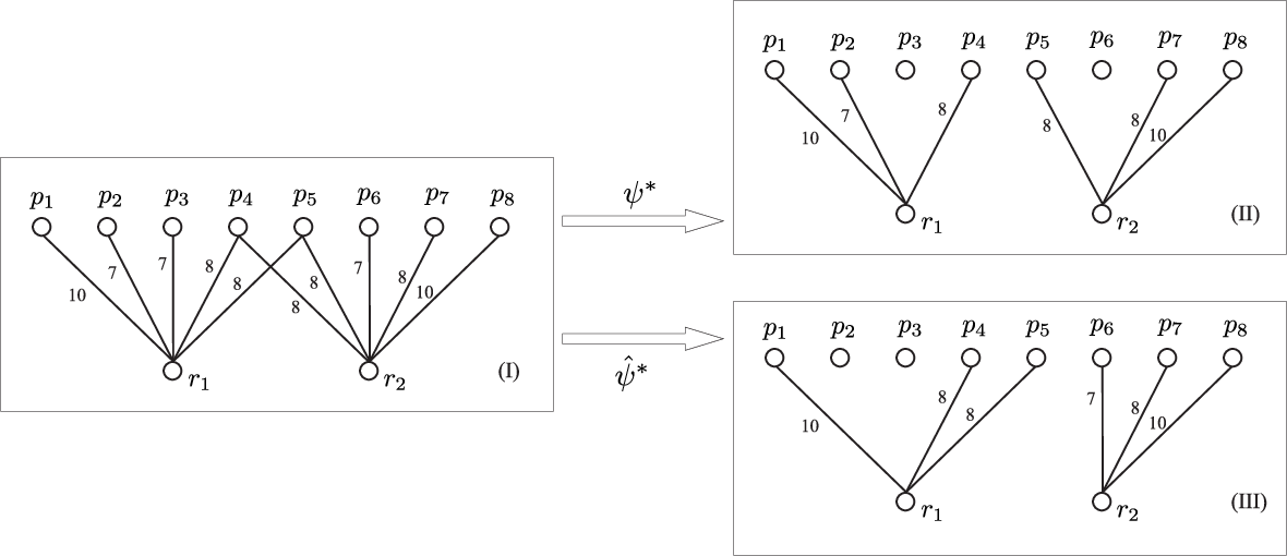
Let us consider the simple scenario that is illustrated in Figure 1(I) by exploiting an intuitive graphical notation. Assume that there are just two researchers, and , affiliated to . Moreover, assume that and , and notice that products and have been co-authored by and . For each (resp., ), let the self-assessed score (resp., ) be the one associated with the edge connecting (resp., ) to . Given this setting, it is then easily seen that an optimal allocation for is such that and —see Figure 1(II).
Let be the optimal allocation being selected by . All products in are then submitted to ANVUR for being evaluated (according to the criteria that are publicly available). As a result of the third phase of the VQR program, each submitted product is associated with a VQR score , which can be in principle different from the score declared by some author . The overall VQR score of the structure , , will be eventually translated to money, proportionally to the performance of w.r.t. the performances of the other research structures. Thus, it is actually immaterial to talk about scores or money in this application scenario.
Example 2.2.
Assume that there is a precise agreement between self-evaluations (leading to the optimal allocation for structure ) and ANVUR evaluations, i.e., for each researcher and each product , holds. Then, we have that —see again Figure 1(II). Moreover, the funds of (actually, the part of funds connected to the research performance) will be directly proportional to . Therefore, if another structure gets 102 as VQR score, its (research-related) funds will be double the funds of .
2.2 Division Rules and Desirable Properties
While the first aim of the VQR program is to evaluate the various Italian research structures, it is known that the obtained information will be used to evaluate substructures, too (e.g., University departments). Thus, following the same principle of binding funds to VQR scores used for the main structures, it is natural to exploit such scores for money distribution inside every research structure (in principle, up to research groups and individuals).
Of course, this poses the question of how the total score (money) of a structure can be fairly distributed over its substructures (and possibly over individuals), in such a way to reflect their actual contribution to the result achieved by the structure. Formally, we need the definition of a division rule , that is, of a real-valued function that given a researcher and an allocation , returns the score of under . Then, slightly abusing notation, for any substructure (here just viewed as the set of its members), denote by the value .
Surprisingly, no division rule has been formalized in the assessment program, up to now, and this is a source of confusion in many researchers. As a matter of fact, most researchers believe that the score of substructures will be based on the naive rule, where for any researcher , is the sum of the VQR scores of the products allocated to in , i.e., . For instance, in the setting of Example 2.2, we have that and . In fact, on the one hand, this approach trivially satisfies a desirable property of division rules.
- (P1) “budget-balance”:
-
A division rule must completely distribute the VQR score of over all its members, i.e., .
However, on the other hand, might lead to scenarios where some researcher (and in turn some substructure) may have some reasonable argument against her/his structure because of possible alternative allocations where that researcher may get a higher score. Indeed, does not satisfy the following:
- (P2) “fairness”:
-
A division rule should assign to each researcher the best score among all possible allocations, i.e., for each , , for any allocation .
Example 2.3.
In fact, to design a division rule satisfying the above (rather strong) fairness criterium is not straightforward. Indeed, property (P2) basically tells us that there must be exactly one possible way to distribute the score over the members of , independently of the optimal allocation being actually selected. Of course, difficulties emerge in those cases where products have multiple co-authors. Thus, to address this issue, one may find natural to consider and analyze the following two division rules:
- :
-
assign to each author the sum of the “normalized” scores of the submitted products (s)he has co-authored, where by normalization we just mean here dividing the score of any product by the number of its authors. For instance, in the setting of Example 2.2, we have that, in the optimal allocation of Figure 1(II), half of the score associated with (equivalently, ) is given to , and the remaining half to . However, even this attempt of having a fair division rule is unsuccessful: The setting of Example 2.3 already evidences that this approach does not satisfy property (P2): just check that while . Indeed, according to this division rule, the score of each researcher depends on the number of publications (s)he has coauthored and has submitted to ANVUR, which may be very different in the various allocations.
- :
-
distribute the score to the members of proportionally to their overall production, and not just on the basis of the submitted publications. Accordingly, for any researcher , we define
In fact, note that satisfies property (P2), precisely because the division does not depend on the specific products being selected and submitted to ANVUR.
Actually, we point out here that, while being conceptually simple and still satisfying the fairness requirement, would be hardly implementable in practice. First, under , it is clear that researchers might want to act strategically and overestimate the quality of their own products. Second, even if is adjusted in a way that it would be always convenient for each researcher to be truthful, we believe that such a theoretical guarantee would still not suffice to create a consensus on the division rule, given that it strongly depends (also) on scores that are not certified by ANVUR. Thus, the specific application scenario we are considering suggests the following additional requirement, which is not satisfied by :
- (P3) “implementability”:
-
A division rule must be indifferent w.r.t. the scores (possibly cheats) declared for unverified products, that is, for products not occurring in the selected allocation.
So far, none of the proposed examples of division rules emerged to be acceptable. Moreover, in our discussion, we have anticipated another crucial requirement for a division rule, which is truthfulness. Indeed, depending on the specific division rule being selected, co-authors may be competitors and might want to act strategically to improve their own score. In particular, while it is clear in principle that the total value of the products should be maximized (social welfare), authors’ personal interest may lead to choices going in a different (non-optimal) direction. Thus, a division rule must prevent manipulation:
- (P4) “truthfulness”:
-
A division rule must provide no incentive in misreporting the score of the research products.
Very recently, (perhaps) having recognized that the research programme might provide incentive to strategic behaviors, ANVUR pointed out that only aggregated information about substructures will be made available, rather than the individual scores of the researchers. However, note that this is not satisfying for two reasons.
First, it is clearly a waste of money to conduct such a thorough evaluation of the quality of the Italian research, without then providing the output of the results for research products. Indeed, this kind of information would be useful to define the part of the salary of each researcher that is function of her/his productivity, according to the current law.33 3 Actually, this applies only to tenured positions at Universities. This is so evident that many researchers still believe that such an information will be used for their personal evaluation (soon or later), and thus are adopting strategic behaviors to have allocated the best products (usually, under the assumption that the rule will be used). However, this might not lead to the global optimum for their research structure, because of possible poor performances of co-authors, as we shall see in the example below.
Second, disclosing only aggregated information does not prevent at all the emergence of strategic behaviors. Indeed, such strategic issues still emerge as soon as two researchers from different substructures co-authored some research product, with each of them being interested in providing as much as contribution as possible to her/his own substructure. Again, this might not lead to the global optimum, as we next exemplify for the rule .

Example 2.4.
Assume that and belong to different substructures. Consider the rule , and assume that researcher declares that her/his products and are of poor quality (e.g., ), as it is illustrated in Figure 2(I). Then, an optimal allocation is the one shown in Figure 2(II), where the set of products is submitted to ANVUR. Assume that, for all these products, there is an agreement between declared scores and ANVUR ones. It follows that . On the other hand, recall that in the allocation of Figure 1(II), which has been computed based on the declaration that , it holds that . Thus, finds convenient to misreport the true scores of and , and underestimate them. Note however that the overall score of the structure is still and, in fact, coincides with the optimal allocation depicted in Figure 1(III) and discussed in Example 2.3.
Then, consider a slight variation of the problem instance depicted in Figure 2 where the actual value of product is (instead of ). Then, the above egoistic behavior of agent also damages its research structure because it leads to a sub-optimal allocation. Indeed, due to the low declared values for and , product is selected and allocated to in the unique (wrong) optimal allocation, whose total score is now (instead of ).

Analogously, the emergence of strategic issues with the rule can be easily seen.
Example 2.5.
Assume again that and belong to different substructures. Consider now the rule , and assume that researcher declares that . Then, consider the optimal allocation shown in Figure 3(II), and note that, in this case, the set of products is submitted to ANVUR.
Now, assume that the VQR scores of these products are those illustrated in Figure 1(I), i.e., the same ones as those discussed in Example 2.1. Thus, has cheated with the aim of overestimating the products of which (s)he is the sole author. In fact, this is convenient to her/him, since according to the rule , now gets , because of the products in allocated to her/him (with overall score 24) and of the product co-authored with (whose overall score is then shared with ). On the other hand, just recall that in the allocation of Figure 1(II), which has been computed based on the “truthful” declaration that , it holds that . It follows that finds convenient to cheat under , in order to increment the number of products submitted to the VQR that (s)he has coauthored. However, the egoistic behavior of agent again damages its research structure, as we now have that the total VQR score is 50 (instead of 51)—see again Figure 3(II).
As a matter of fact, the emergence of strategic issues across substructures risks to penalize, in the long term period, collaborations and cross-fertilizations.44 4 It is not by chance that the authors of this paper belong to different substructures of the same University. To prevent all these problems, a truthful mechanism is of course definitively needed. In fact, as the above examples might have already suggested to the careful reader, truthfulness can be achieved by exploiting the fact that ANVUR evaluation corresponds to a “verification ability” available in the setting. For instance, one might punish (e.g., by assigning 0 as overall score) all those researchers whose reported values are found different from the verified ones (usually interpreted as “lying agents”), as it is in the spirit of most of the literature on mechanisms with verification (see, e.g., ?, ?, ?, ?, ?). Indeed, under the intimidation of a punishment, any (reasonable) division rule can be turned into a truthful one. However, in the application scenario we are considering, a punishment approach would be hardly “politically” acceptable—just think that a number of researchers have already announced that they will not participate to the VQR program because they disagree with some of the evaluation criteria made available by ANVUR, which are in fact perceived as imposed by “law” rather than as being the outcome of a public discussion on the subject. Moreover, charging researchers because of some discrepancy between their self-evaluation about some paper and the one by ANVUR experts would require some convincing proof of their malicious behavior. Therefore, any punishing approach would be quite hard to implement in practice, for this real-world case study. For this reason, we avoid this brute-force approach, and ask that the following property holds.
- (P5) “no punishment”:
-
A division rule must be such that, for each and each allocation , the value is indifferent w.r.t. self-assessed scores, in particular, w.r.t. discrepancies possibly emerging between such scores and VQR ones.
Note that, in the light of the above requirement, we look for a method to enforce truthfulness where verification is used in a rather limited sense. Moreover, it is relevant to observe that if the division rule is not well-designed, then cases might emerge where there is no way at all to exploit verification (even in its strongest form where punishment is allowed).
Example 2.6.
Consider again the use of the rule in Example 2.4, and recall that finds convenient to underestimate the true scores of and . However, since and does not occur in , as we can see in Figure 2(II), then there is no way to discover that has actually cheated. Therefore, in this case, verification on the selected products provides no-extra power, and truthfulness is not achieved.
3 Fair Allocation Problems
By looking at the examples discussed in the above section, it emerges that defining a “good” division rule is not an easy task in allocation problems with indivisible goods.
In this section, we provide the formal framework for studying such problems, based on mechanism design tools. In particular, we focus on mechanisms equipped with a verification ability, which meets the “no-punishment” perspective. To help the intuition, after notions are defined in the formal framework, we discuss how they fit our running (motivating) example about the Italian research assessment programme.
3.1 Formal Framework: Allocations and Strategic Setting
Assume that a universe of indivisible goods is given. An allocation scenario over is a tuple where is a set of agents, is a set of goods, and is a function associating each agent with a natural number .
An allocation for is a function mapping each agent into a set of goods with and such that , for each agent . Note that provides the upper bounds on the number of goods that can be allocated to agents. Of course, this is more general than assuming that no bound is given, which is just the special case , for each agent . Eventually, note that goods cannot be shared. In the following, we denote by the domain of , and by the set of goods occurring in the image of , that is, .
The type of an agent is a real-valued function over , which is meant to express her/his evaluation of each single good. A vector where is the type of agent , for each , is called a type vector. The value of an allocation for w.r.t. , denoted by , is given by . Then, is optimal (for w.r.t. ) if there is no allocation for such that . The value of an optimal allocation for w.r.t. is denoted by , while the set of all optimal allocations for w.r.t. is denoted by , or simply by if is understood from the context.
For each agent , let be the set of all her/his possible types, and let be the Cartesian product . Hereinafter, we assume that an allocation scenario is given, together with two type vectors and . In particular, we assume that each agent reports a declared type , which might be different from her/his actual evaluation of the available goods, called the true type of . Vector is public knowledge, while vector is not, because type is private knowledge of agent .
Allocation problems VQR. The motivating scenario discussed in Section 2 is a special case of the above general framework. Indeed, we can associate each structure with an allocation scenario , where is the set of researchers affiliated to , is the set of their products, and is the constant function stating that each researcher can submit 3 products at most. In this setting, encodes the scores declared by the researchers (with the negative score being conventionally assigned by to the products that declares not to have authored). This correspondence is exemplified below.
Example 3.1.
Consider again the setting of Example 2.5. The given research structure can be modeled as the allocation scenario . Moreover, the vector is such that, for each and : , if , and , otherwise. Note that Figure 3(I) can be viewed as a graphical representation of where negative edges are omitted. For instance, for researcher , we have , , , and so on. Clearly, optimal allocations for the research assessment problem one-to-one correspond to optimal ones for the corresponding allocation scenario w.r.t. . For instance, the allocation in Figure 3(II) is an optimal allocation for w.r.t. .
Concerning the vector of true types in the VQR setting, recall that research products are evaluated by ANVUR according to some publicly available criteria, and that, having such criteria, every author is expected to be able of self-evaluating her/his own products in a way consistent with ANVUR evaluation. Thus, the vector encodes the “true score” of each product, as it can be determined according to ANVUR evaluation criteria.
Actually, note that in the case of the VQR setting, different researchers cannot have truly different true types w.r.t. a product they have co-authored, because we are assuming that true types coincide with ANVUR evaluations and ANVUR provides just one value for each product. More formally, in any VQR allocation problem , the underlying vector of true types is such that and implies that , for each good and pair of agents . Of course, since the proposed framework is more general, it may well support possible extensions of the current VQR setting tailored to a finer-grained analysis of interdisciplinary products. Indeed, for such products, co-authors can actually have different valuations for the same paper (e.g., for they belong to scientific communities with a different research focus) and, therefore, it makes sense to have the product reviewed by a different panel of experts for each author/area of interest.
3.2 Mechanisms with Verification
Throughout the paper, we consider mechanism design in a setting where a third-party, called the verifier, is formalized as a function associating any allocation with a vector of verified types, with , for each agent . In particular we assume that, for each agent and good , . Note that a verifier is always able to precisely determine the real value (agents’ type) of any good in , i.e., of any good allocated to some agent by . Thus, in our setting, values for allocated products can be fully verified. Instead, is undefined over values that are not allocated, and hence not verified.
In order to encourage agents to truthfully report their private types, we shall design mechanisms where monetary transfers can be performed, after verified types are available. Formally, a payment rule is defined as a vector of functions, with being some amount of money that is given to agent , on the basis of an allocation and a vector . Observe that, with this notation, any negative value means that some amount of money is charged to agent . Then, ’s (quasi-linear) utility under , sometimes called individual welfare, is defined as . Whenever the payment rule is easily understood from the context, ’s utility is simply denoted as . Note that utilities depend on verified types, as in the setting by ? (?). In fact, we could have equivalently stated them in terms of the true types. However, the proposed formulation best reflects the intended meaning of the framework, where payments—and hence utilities—depend on the verification process rather than on personal beliefs of agents.
An allocation algorithm is a function mapping each vector into an allocation . We say that the algorithm is optimal if , for each .
A mechanism with verification is a pair , where is an allocation algorithm and is a payment rule that can exploit the power of a verifier . The mechanism can be viewed as consisting of the following two-phases: First, agents report a declaration vector , and an allocation is computed, by using some allocation algorithm . Second, the true types “restricted” over are revealed, i.e., is made available, and payments under a given rule are calculated for and , by exploiting the knowledge of . Intuitively, our goal is to design a payment rule guaranteeing that declared types in induce an allocation maximizing the social welfare, i.e., such that holds. A comparison of our approach to verification with existing ones is reported in Section 7.
Allocation problems VQR. In the VQR setting, we have already pointed out that ANVUR precisely plays the role of a verifier. For instance, by considering again Example 2.5, we have that the set is submitted to ANVUR and hence, for instance, , because product of has been verified and hence ’s evaluation about it has been disclosed—see also Figure 3(II). Moreover, negative values model the types of researchers for products that cannot be assigned to them. E.g., we have , because is not an author of , which is always trivially checked by the mechanism (note that the specific negative value is immaterial).
Our goal is then to single out a mechanism with verification that uses appropriate “monetary” transfers to compensate the (globally) optimal allocation of the given indivisible goods. In particular, note that, in order to be consistent with the quasi-linear setting, payments in the VQR setting have to be intended as redistributions of the VQR overall score . As a result, the role of a division rule is now to determine the individual welfare associated with each researcher/agent . In fact, payment rules should guarantee that welfare values satisfy a number of desirable properties, in particular, the relevant ones pointed out in Section 2.
As a further remark, note that our choice of making the dependence on verified types explicit in the definition of the utility function is conceptually clearer than assuming a dependence on true types (in fact, eventually coinciding with verified ones). Indeed, our choice is adherent to the VQR setting, where funds (the actual utility of each researcher) will be determined according to ANVUR evaluations.
3.3 Properties of Mechanisms
For any vector of types (declarations) and for any type , we denote by the type vector .
Let be a mechanism with verification, and let by any agent in and her/his declared type. We say that is a dominant strategy of agent w.r.t. if, for each vector , holds.
The mechanism is truthful if, for each , is a dominant strategy. This is in fact property (P4) in Section 2. Let be any truthful mechanism. In the paper, we will also focus on the following standard (ex-post) properties of such a mechanism, to be checked at the equilibrium where agents truthfully report their private types:
-
efficiency: . That is, the social welfare is maximized.
-
individual rationality: , for each agent . Hence, voluntary participation is encouraged.
-
(strong) budget-balance: . In other words, there is no transfer of money out of or into the mechanism. This is in fact property (P1).
-
envy-freeness: for each pair of agents , and for each allocation such that , .
-
Pareto-efficiency: there is no allocation such that: (1) , for each agent , and (2) there is an agent with . That is, is not Pareto-dominated by any other allocation.
Note that envy-freeness and Pareto efficiency are two direct consequences of the much stronger property (P2), which can now be formalized as follows:
-
fairness: , for each agent and for each allocation .
The two remaining properties (P3) and (P5) from the list in Section 2 (“implementability” and “no punishment”, respectively) will be considered as well. Note that these properties must hold in general, i.e, not only at the equilibrium. In fact, in the more general setting of allocation problems, they can be respectively formalized as follows:
-
implementability: , for each agent , for each allocation , and for each pair of vectors that that may differ only outside , i.e., , for each and . That is, goods that are not allocated and hence not verified do not play any role in payments.
-
no punishment: , for each agent , for each allocation , and for each type vector . That is, the payment function for agent does not depend on her/his declared values, so that possible discrepancies with the verified type do not affect ’s payment according to the given allocation. In other words, we may think of payments being always computed under the presumption of innocence, where incorrect declared values do not necessarily mean manipulation attempts by the agents.
4 Mechanisms with Verification for Allocation Problems
In this section, we introduce a mechanism with verification for allocation problems and start its analysis, by preliminary evidencing some properties that hold over optimal allocations.
4.1 General Properties of Allocation Problems
We first observe that the optimization problem used to allocate goods to agents can be equivalently reformulated in such a way that at most one good can be allocated to each agent. Intuitively, we may replace each agent by fresh agents with the same properties as . We remark that such an equivalence is just used for the combinatorial optimization phase, i.e., without taking into account any (game theoretic) incentive consideration.
Let be an allocation problem. We denote by its one-good version , where is the set of agents such that for each agent , is a set of fresh agents, and where is the constant function mapping each agent to . For any vector mapping each agent in to her/his type, let be the type vector for agents in such that , for each and . Thus, in the allocation problem and considering the type vector each “clone” can get at most one good, and it has the same valuations as agent in .
Example 4.1.
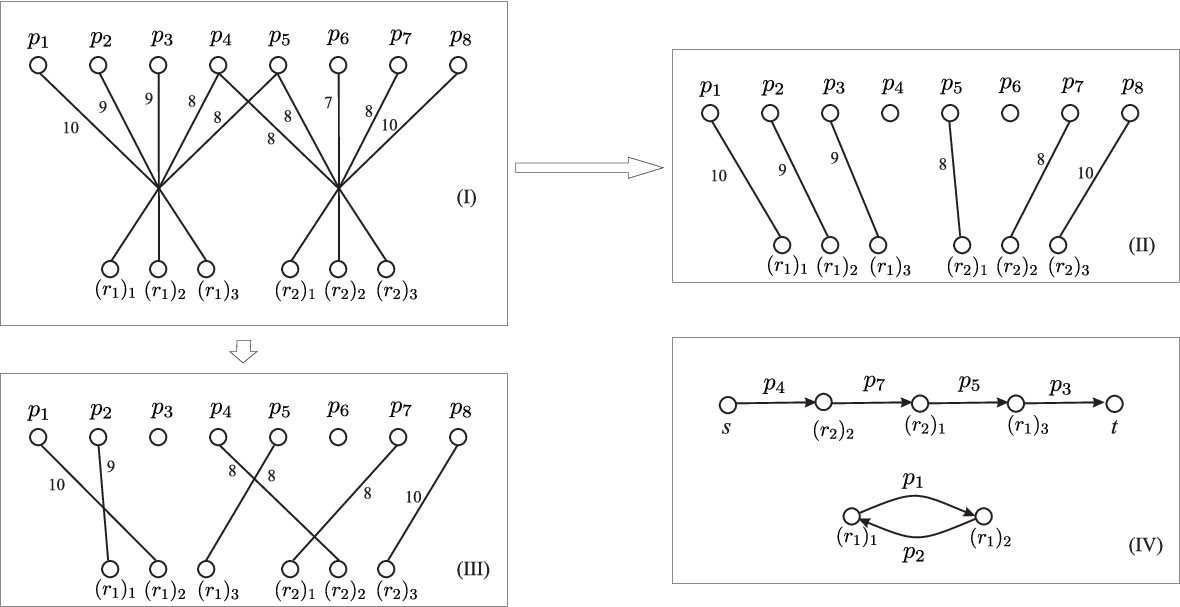
Consider again the ANVUR scenario discussed in Example 2.5 and illustrated in Figure 3. Recall from Example 3.1 the associated allocation problem , with . Moreover, recall that the vector of declared types is such that, for each and : , if , and , otherwise. Its one-good version is shown Figure 4(I), where the set of agents is and where we have that (resp., ), for each . In this graphical representation, crossing lines represent the edges of the bipartite cliques connecting the two groups of virtual researchers with their products, while, as usual, edges with negative scores (valuations for products owned only by other authors) are omitted.
For any set of agents and set of goods, the tuple is the restriction of where only agents in and goods in are considered.55 5 Note the little abuse of notation: the function in should be in fact its restriction over . However, to keep the notation simple, we just write , as no confusion may arise. Similarly, any type vector for will be transparently considered as a type vector for any subset of agents —we just get rid of the unused components associated with agents in . Consider such a scenario and let be an allocation for its one-good version . Note that induces the allocation for , denoted by . By construction, . Conversely, any allocation for is associated with the non-empty set of all those allocations such that , also called the one-good forms of .
Fact 4.2.
Let be an allocation problem, let be its one-good version, and let be an allocation for . Then, is an optimal allocation for w.r.t. if, and only if, is an optimal allocation for w.r.t. .
Example 4.3.
We are now in the position of stating a property that holds on any optimal allocation . The property is in fact of interest of its own, i.e., independently of its application to the design of a mechanism with verification. In words, it tells us that, whenever we are interested in allocating goods to any subset of agents, we may safely consider only goods in , rather than the whole set . In our case, it is a basic technical ingredient for showing a number of key properties because, intuitively, it allows us to get rid of alternative (optimal) allocations, possibly based on non-evaluated goods in .
Theorem 4.4.
Let be an optimal allocation for w.r.t. , and let be the set of goods allocated according to . Then, for each set of agents , every optimal allocation for w.r.t. is an optimal allocation for w.r.t. .
Proof.
Let be any set of agents, and let be any optimal allocation for w.r.t. , where . We show that is an optimal allocation for the unrestricted problem w.r.t. , too.
To this end, consider any optimal allocation for the problem where all goods in are available to the agents in . We next prove that . This clearly follows from the optimality of if holds. Therefore, to be strictly better than , a function must allocate some good in . Assume thus by contradiction that , and hence , which entails that . Consider two allocations and , and observe first that:
Let be the set of agents whose good-assignment are the same according to these allocations, i.e., . Then, define to be the directed graph, called update graph for w.r.t. , whose nodes are the agents in that change their goods in the two allocations plus two distinguished nodes and , and whose edges in are defined as follows:
-
There is an edge from agent to agent if ;
-
There is an edge from to agent if there is no agent such that ;
-
There is an edge from agent to if there is no agent such that ;
-
No further edges are in .
For an example construction, consider Figure 4(IV) showing the update graph for the allocation shown in Figure 4(II) w.r.t. the allocation shown in Figure 4(III).
As each agent gets at most one good in and , each node in but and has exactly one incoming edge and one outgoing edge. Moreover, by construction, has no incoming edge, and has no outgoing edge. Thus, the update graph consists of a number of paths from to and a number of cycles, all of them being disjoint from each other.
Let be the set of all possible paths from to or cycles in , and for a path or a cycle , let be the set . In addition, let us fix the following notation: For any function , let denote the restriction of over . Moreover, for the functions and with , let be such that and .
By the construction of the update graph, note that can be expressed in terms of the disjoint paths/cycles by the following expression:
Because , there must exists a set of agents , associated with some disjoint path/cycle , with , such that the value of the goods allocated to these agents according to is greater than the corresponding value for the same agents obtained after . That is, the function , which is an allocation for , is such that . Note that if were a cycle or a path of the form such that , then would hold. Indeed, only the first node in a path, such as , may be such that . However, as observed above, this is impossible because would contradict the optimality of , and hence the optimality of , by Fact 4.2.
Therefore, we can conclude that is a path of the form with . That is, the allocation (over the agents in ) is such that . In particular, observe that .
Let us now come back to the optimal allocation for w.r.t. , and let be an (optimal) allocation in . Let be a set of agents with such that the set of goods allocated to these agents according to is equal to where and . Note that a set having this property in fact exists: just start with and then add agents from until some is found with .
Consider then and note that is indeed an allocation for , because the construction of the set guarantees that no good allocated according to can be allocated by to agents in , and vice-versa. Since is an optimal allocation for w.r.t. , holds. Thus, by construction of , we get .
Finally, let and note that is an allocation for . Moreover, observe that and . For this latter, just recall that is the only agent in such that . Again, this entails that is not optimal w.r.t. and hence by Fact 4.2 is also not optimal for w.r.t. . Contradiction. ∎
The result immediately entails the following two corollaries.
Corollary 4.5.
For each optimal allocation for w.r.t. and for each set of agents, .
Corollary 4.6.
Let be an optimal allocation for w.r.t. , and let be any allocation for , hence with . Then, for each set of agents, .
Input: An allocation for , and a vector ; Assumption: A verifier is available. Let ; 1. Let denote the set of all possible subsets of ; 2. For each set , 3. Compute an optimal allocation for w.r.t. ; 4. For each agent , 5. For each set , 6. Let ; (=); 7. Let ; (=); 8. Let ; 9. Define ;
4.2 The Design of a Truthful Mechanism
With the above notation and results in place, we can now discuss the payment rule that is illustrated in Figure 5: We are given an allocation that selects some goods for the agents in , plus a vector . Moreover, we assume the existence of a verifier computing the vector .
In the first three steps, the payment rule associates an optimal allocation for w.r.t. with each set of agents, where is the powerset of , i.e., the set of all possible subsets of agents. Then, for each agent and for each set , we define two terms, namely and , which evaluate the allocations and under the assumption that agent types are and , respectively. These terms will play a role in the definition of the value at step 8. In particular, we observe that the definition of this value is reminiscent of the definition of the Shapley value, as it considers the marginal contribution of each possible set summed up in a weighted manner w.r.t. its size.66 6 The reader that is not familiar with this solution concept is referred to the introductory part of Section 5, where the Shapley value is formally defined. Finally, the payment is defined at step 9 as the difference between and .
Note that the idea underlying the definition of is that, after verification is performed, the utility function will precisely coincide with the “bonus” , hence sharing the spirit77 7 In fact, the peculiar form of does not fit the general schema by ? (?). of the approach by ? (?). Indeed, the following is immediate.
Lemma 4.7.
For each allocation for , for each vector , and for each agent , it holds that .
By exploiting this characterization, we can now show the first crucial result on the payment rule , i.e., that the mechanism —where is any arbitrary optimal allocation algorithm—is truthful.
Theorem 4.8 (truthfulness).
Let be any optimal allocation algorithm. Then, the mechanism with verification is truthful.
Proof.
We have to show that, for each agent , and reported type vector , the following holds: ; hence, by Lemma 4.7, that .
Consider the construction reported in Figure 5 for the two cases of and , and let and be the corresponding allocations (optimal w.r.t. and , respectively) received as input by the payment rule in Figure 5. For any set of agents, let (resp., ) be the allocation computed at step 3. We show that the following two properties hold, for each set of agents :
- (A)
, and
- (B)
.
In order to prove (A), observe that by step 6, , because in this case reports the actual private type , which is equal to the verified one. Now, recall that is an optimal allocation for w.r.t. , and is an optimal allocation for w.r.t. . Thus, by Corollary 4.5,
| (1) |
Similarly, . In this case, observe that the reported type of is , which is different from . Also, is an allocation for , hence it allocates goods in , for which the true type is revealed in . Thus, we may compute .
In order to conclude, let us note that is an allocation for , though it is not necessarily optimal w.r.t. . Thus, by using Equation 1, . This shows that (A) holds.
Let us now focus on (B). By step 7, we preliminary observe that we have and . Then, recall that is an optimal allocation for w.r.t. and is an optimal allocation for w.r.t. . Thus, by Corollary 4.5, and because ’s evaluation is immaterial here, we get (B) as follows: ∎
In addition to truthfulness, it suddenly emerges that the payment rule is indifferent w.r.t. deviations from the actual values (possibly, cheats) on goods that do not occur in the allocation being selected. We have already observed that this property is relevant in our motivating scenario, where payments should be made only with respect to certified goods (as evaluated by a third-party agency). Now, we state it in formal terms.
Theorem 4.9 (implementability).
For each allocation for and for each agent , it holds that , for each pair of vectors that differ only outside .
Proof.
It suffices to observe that, in the algorithm in Figure 5, optimal allocations are restricted over the set at step 3. Thus, the payment rule is completely indifferent w.r.t. agents’ evaluations of the goods outside . ∎
Moreover, it can be noticed that payments do not depend on possible discrepancies between declared and verified values, as shown below.
Theorem 4.10 (no punishment).
For each agent , for each allocation for , and for each type vector , it holds that .
Proof.
Recall that, in the algorithm in Figure 5, only goods in are considered, and observe that the payment for agent depends only on her/his verified type, rather than on the declared one. ∎
4.3 Further Properties of Truthful Strategies
Let us now analyze some relevant properties that hold on whenever agents choose their dominant strategy of truthfully reporting their private types. The first property is a useful characterization for the utility of the agents.
Theorem 4.11.
For each optimal allocation for w.r.t. , and for each agent , it holds that:
Proof.
By Lemma 4.7, we know that . Then, for each set of agents, and for each agent , consider the expressions and defined at step 6 and step 7, respectively, of the mechanism in Figure 5. Note that and , where and are optimal allocations for w.r.t. and for w.r.t. , respectively. Thus, and . It follows that:
| (2) |
Note that in the above expression, agents’ utilities are completely independent of the particular optimal allocation . Therefore, in every optimal allocation, every agent gets precisely the same utility.
Corollary 4.12.
Let and be two optimal allocations for w.r.t. . Then, holds, for each .
Example 4.13.
Consider the allocation scenario , where , associated with the research structure in Example 2.1. Assume that researchers declare their true types in the ANVUR evaluation, and consider the optimal allocation shown in Figure 1(II). Then, we have:
In particular, note that , as we can allocate , , and to , if (s)he where the only researcher in the structure.
Similarly, we get . That is, the two researchers will share precisely one half of the total score of their structure, based on our payment scheme. In fact, by looking at the allocation in Figure 1(II), one might naïvely suppose that contributed more than . However, this is only due to the specific allocation considered, and not to the actual values of the products of the two authors. For instance, is allocated to but it was produced by , as well. Indeed, the fairness of the utility values resulting from our payment rule suddenly appears when considering the alternative allocation in Figure 1(II), which is symmetric w.r.t. and where it seems that contributes more than : As a matter of fact, the two researchers are completely interchangeable over optimal allocations, and this is correctly reflected by our payment scheme. In particular, from Corollary 4.12, the researchers are indifferent w.r.t. the specific optimal allocation being selected, and hence in this case they equally divide all the available score between themselves.
We conclude by pointing out a further important property of the mechanism.
Corollary 4.14 (individual-rationality).
Let be any optimal allocation algorithm. Then, the mechanism with verification is individually-rational.
Proof.
Notice that , holds for each and agent . Then, by Theorem 4.11, holds, for each agent . ∎
5 A Coalitional Game Theory Viewpoint
A coalitional game can be modeled as a pair , where is a finite set of agents, and is a function associating with each coalition a real-value , with , which is meant to encode the worth that agents in obtain by collaborating with each other. The function is supermodular (resp., submodular) if (resp., ) holds, for each pair of coalitions .
A fundamental problem for coalitional games is to single out the most desirable outcomes, usually called solution concepts, in terms of appropriate notions of worth distributions, i.e., of vectors of payoffs such that . This question was studied in economics and game theory with the aim of providing arguments and counterarguments about why such proposals are reasonable mathematical renderings of the intuitive concepts of fairness and stability. For further background on coalitional games, the reader is referred to, e.g., (?).
Here, we consider the Shapley value of , which is a well-known solution concept such that:
Indeed, we shall show that the mechanism defined in Section 4 has a nice interpretation in terms of the Shapley value of some suitable-defined coalitional games. The correspondence will be exploited to prove further properties of our mechanism.
5.1 The Shapley Value of Allocation Games
We consider two coalitional games defined on top of an allocation problem.
Definition 5.1.
Given the tuple and a vector of agent types, we define and as the coalitional games such, that for each set of agents,
-
; and,
-
.
Note that is the marginal contribution of to . Instead, is the best contribution of (w.r.t. ), computed assuming that agents in were the only agents in the allocation problem. In particular, the game has already been considered by ? (?), precisely in the setting of fair division for allocation problems. There, it is shown that the cost function associated with is submodular.
Proposition 5.2 (? (?)).
The function is submodular.
Then, the (dual) analogous for can be shown easily.
Theorem 5.3.
The function is supermodular.
Proof.
Let be the given structure, and be a vector of types. The result just follows by noticing that , for each set of agents . That is, . Thus, if holds , we have that holds as well, . Eventually, by letting and , we get , for each . That is, is supermodular. ∎
As a second relevant property, we next observe that the payment rules in Section 4 coincide, at the equilibrium where agents truthfully report their types, with the Shapley value of the game associated with . The result follows by comparing the utility function as in Theorem 4.11 with the expression for the Shapley value of the coalitional game . Moreover, we show that the same result can be established for the “dual” game , so that the Shapley values of the two games are identical—for similar correspondences between Shapley values of different games, see also the works by ? (?) and ? (?).
Theorem 5.4.
For each optimal allocation for w.r.t. , and for each agent , it holds that .
Proof.
By comparing the utility function as in Theorem 4.11 with the expression for the Shapley value of the coalitional game associating with each coalition of agents the worth , we immediately get that, for each optimal allocation for w.r.t. , and for each agent , it holds that .
In order to conclude the proof, we show that for each agent , holds. To this end, first note that these Shapley values can be written as follows:
-
, and
-
,
where and
Then, we claim that:
- (1)
for each set of agents with , the set is such that , and
- (2)
for each set of agents with , the set is such that .
(1) Let such that , and observe that . Thus, let , and note that .
(2) Let such that , and observe that . Thus, let and note that .
As (1) and (2) hold, and given the two expressions for and , we conclude that the two values coincide. ∎
5.2 Fairness and Budget-Balancedness
Now that we have established a precise correspondence between our mechanism and the Shapley value of its associated allocation games, we can show further desirable properties of . In fact, we exploit the following well-known properties (see, e.g., ?, ?) of the Shapley value of any game :
- (I)
;
- (II)
If is supermodular (resp., submodular), then (resp., ).
- (III)
If is a game such that , for each , then , for each agent .
Our first result is to show that and provide an upper and a lower bound, respectively, to the sum of the utility functions over any set of agents. This is particularly useful whenever we have to reason in terms of fairness for groups of agents, rather than just in terms of the utility of singletons.
For instance, in the motivating scenario of Section 2, a crucial question concerns how the structure funding after the ANVUR evaluation (e.g., the research funds for a University) should be shared among its sub-structures (e.g., the Departments). The result below shows that, with our mechanism, any sub-structure will never get less than its marginal contribution, neither more than the maximum contribution it can achieve if its members were alone in the structure. In particular, any closed group of researchers (e.g., any department without collaborations with other departments, or any research group without further coauthors in the same structure) will share precisely the total value attributed by ANVUR to its research products. Such a score is desirable for agents, and it is perceived as a fair distribution (see the work by ? (?), for more on the fairness of the Shapley value).
Theorem 5.5.
Let be an optimal allocation for w.r.t. . Then, for each set of agents, .
Proof.
Our second result pertains the budget-balance property of the mechanisms. Again, the correspondence with the Shapley value is crucial to establish the result.
Theorem 5.6.
Let be an optimal allocation for w.r.t. . Then, it holds that .
Proof.
By Theorem 5.4, we know that , for each agent and optimal allocation , where is the Shapley value of . By property (I) of the Shapley value, we know that . Thus, . It follows that , by definition of the utility. Hence, , as is indeed an optimal allocation w.r.t. (and, hence, w.r.t. verified types). ∎
Corollary 5.7 (budget-balance).
Let be any optimal allocation algorithm. Then, the mechanism with verification is budget-balanced.
Finally, we complete the picture of our analysis by proving the strong fairness property of the proposed payment rule : In words, the best outcome for every agent is always determined by a (global) optimal allocation. Moreover, from Corollary 4.12, any agent is indifferent about the specific optimal allocation being considered. That is, any chosen optimal allocation leads to the best results for all agents.
Lemma 5.8.
Let and be two allocations for such that is optimal, and hence . Then, holds, for each . Moreover, if is not optimal, there exists some agent such that .
Proof.
For any allocation , consider the coalitional game such that , for each . By looking at the expression of the Shapley value for , it is easy to check that (just use the same reasoning leading to Equation 2 in the proof of Theorem 4.11). Assume now that is an allocation with , and consider the value , for each . By Corollary 4.6, we have that , for each . Then, we derive that for every , because of property (III) of the Shapley value.
Now assume that is not optimal, and thus . Therefore, for the grand-coalition , we have . Because of property (I) of the Shapley value, only (and all) the total value is distributed to agents. It follows that there exists some agent such that . ∎
Because, truthful declarations lead to optimal allocations, the desired fairness property is immediately entailed by the previous lemma.
Theorem 5.9 (Fairness).
Let be any optimal allocation algorithm. Then, for any agent and any allocation , .
Corollary 5.10 (Pareto-efficiency and envy-freeness).
Let be any optimal allocation algorithm. Then, the mechanism with verification is Pareto efficient and envy-free.
Note that the above fairness condition guarantees much more than classical Pareto efficiency and envy-freeness, because it entails that the mechanism leads to a unique evaluation, independently of the chosen optimal allocation. In particular, the Pareto set is a singleton.
6 Complexity Issues
In this section, we shall reconsider our mechanism with verification from a computational perspective. Note first that computing an optimal allocation on the basis of the reported types is an easy task, which can be carried out via adaptations of classical matching algorithms. Indeed, in the light of Fact 4.2, computing an optimal allocation for reduces to computing an optimal allocation for w.r.t. , which is a scenario where each agent can be allocated one good at most. This is equivalent to find a matching of maximum weight over a complete bipartite graph over the set of disjoint nodes and , and where edge weights are encoded via the function . This task is well-known to be feasible in polynomial time (e.g., ?).
6.1 Hardness Result
Despite optimal allocations can be computed in polynomial time, our mechanism is not computationally-efficient, since payments are unlikely to be computable in polynomial time. Indeed, we next show that this computation problem is complete for the complexity class (see ?).
For the sake of completeness, we recall here that a counting Turing machine is a standard nondeterministic Turing machine with an auxiliary output device that prints in binary notation the number of accepting computations induced by the input. It has (worst-case) time complexity if the longest accepting computation induced by the set of all inputs of size takes steps. Then, #P is the class of all functions that can be computed by counting Turing machines of polynomial time complexity. A prototypical #P-complete problem is to count the number of truth variable assignments that satisfy a Boolean formula. Of course, NP#P, and a polynomial-time algorithm for solving a #P-complete problem would imply P = NP.
Theorem 6.1.
Computing the Shapley value of coalitional games associated with allocation problems (as in Definition 5.1) is #P-complete.
Proof.
The problem belongs to #P, because computing the Shapley value is known to be feasible in #P for any class of coalitional games with polynomial-time value/cost functions (c.f. ?). To show that it is #P-hard, we exhibit a reduction from the following problem: Let be a bipartite graph with , , and . Recall that a matching is a set of edges such that for each pair of distinct edges and in , and hold. The matching is perfect if . The problem of counting the number of perfect matchings in such bipartite graphs is #P-complete (?).
Given a graph as above and a constant (which we shall fix below), we build in polynomial-time a tuple and a type vector such that:
- (1)
, i.e., agents are one-to-one associated with distinct clones of each edge , plus a distinguished node . Note that , because in the considered bipartite graphs holds;
- (2)
, i.e., goods correspond to nodes, plus a distinguished good ;
- (3)
is the function such that , and , for each and ;
- (4)
Types are as follows. For each , , , , , . Moreover, , , .
Let us now fix some notations. For any set of edges, let denote the size of the largest set of edges that is a matching. For any set of agents, let and . Finally, we say that is tight if it does not contain two agents of the form and , with , i.e., associated with the same edge of .
Observe that, for each set of agents,
Indeed, if is an optimal allocation for w.r.t. , then we always have that . Instead, if is an optimal allocation for w.r.t. , then we have
By exploiting Equation 6.1, we can now express the Shapley value of the game for agent in a convenient way. Let denote the number of sets of agents which are tight and such that , and let . Then,
| (6) |
In particular, let us now focus on the coefficient . Denote by the number of matchings in whose cardinality is . By construction of it is immediate to check that for each matching of cardinality in , there are precisely sets of agents that are tight and such that . Thus, we can rewrite the above expression:
| (7) |
For an expression as the one above, given the value of , it is known that under certain circumstances we can reconstruct in polynomial time the value of each single term of the form (see Fact 6 in the work by ? (?)): We need the existence of an integer constant such that, for each , , and . In our case, it can be noticed that, for each , holds, as . Thus, for , we have that, given the value of , we can compute in polynomial time all such terms. In particular, we can compute in polynomial time the term associated to , where recall that . This term has the form , with being the number of perfect matchings in . Thus, by putting it all together and since can be computed in polynomial time (as the size of the numbers and are logarithmic w.r.t. the size of ), the number of perfect matchings in bipartite graphs can be counted in polynomial time too, which concludes the proof. ∎
Corollary 6.2.
Computing the payments as given by the rule is -complete.
6.2 A Fully Polynomial-Time Randomized Approximation Scheme
An approach to circumvent the intractability of the Shapley value is based on approximation: For a game , a vector is an -approximation of the Shapley value if holds, for each .
Recently, a sampling method conceived by ? (?) for the special class of simple coalitional games has been extended to deal with arbitrary games that are supermodular and monotone88 8 Monotonicity of means that , . (?), under the assumption that the value can be computed by an oracle having unitary cost, for each . The result is that, for any and , it is possible to compute in time a vector that is an -approximation of the Shapley value with probability of failure at most . A method with this properties is called a fully polynomial-time randomized approximation scheme.
Input: An allocation for , a vector , and an integer ; Assumption: A verifier is available. Let ; 1. Generate a set of subsets of , and add to them the grand-coalition ; 2. For each set , 3. Compute an optimal allocation for w.r.t. ; 4. Compute an optimal allocation for w.r.t. ; 5. For each agent , 6. Compute as in Figure 5 (steps 4—8), with ; 7. Repeat times steps 1, 2, and 5, and 8. Let be the component-wise median vector of these vectors ; 9. Define ;
Next, we propose a payment rule that is founded on the sampling strategy described in the work by ? (?). The payment rule, reported in Figure 6, samples subsets of storing them in , and then computes the value as in Figure 5, but with playing the role of the power-set . Eventually, the process is repeated times, and the component-wise median vector of all such payments is computed. Finally, at step 9, the usual compensation and bonus approach is implemented.
Interestingly, though the new rule is based on randomization, the following properties still hold (always, not just as expected outcomes).
Theorem 6.3.
Let be any optimal allocation algorithm. Then, the mechanism with verification is truthful and individually-rational.
Proof.
The result follows by inspecting the proofs for rule in Section 4. Indeed, it can be immediately checked that those proofs do not depend on the specific subset of coalitions , and thus they smoothly apply if any set of coalitions is used as in Figure 6, instead of all possible subsets of . Note in particular that, despite the payment rule is based on randomization, the resulting mechanism is always truthful: just look at the proof of Theorem 4.8, and notice that properties (A) and (B) are precisely those guaranteeing truthfulness, and that these properties hold for each given coalition . Therefore, they still hold for any subset of coalitions randomly chosen by the mechanism. ∎
For continuing with a deeper analysis of the payment rule , we need to point out a relationship between utility values and approximations of the Shapley value.
Lemma 6.4.
Let , and let . Then, for each optimal allocation for w.r.t. , the vector is in expectation the Shapley value of (and ), of which it is an -approximation, with probability .
Proof.
By exploiting the same line of reasoning as in the proofs in Section 4 for , we can see that (at step 6 of the algorithm in Figure 6) can be rewritten as follows:
Now, recall that the game is supermodular by Theorem 5.3. Moreover, is clearly monotone. Thus, by Theorem 4 in the work by ? (?), we derive the result in the statement, but for the fixed value of . Steps 7 and 8 just serve to amplify the probability (c.f. ?), and to get a fully polynomial-time randomized approximation scheme. ∎
As the expected utility profile coincides with the Shapley value, it is easy to see that enjoys in expectation all the properties of (e.g., Pareto-efficiency and envy-freeness). We thus focus in this section on those properties that can be shown to hold always, i.e., not just in expectation. With this respect, note that in the approach by ? (?), a final normalization step is carried out to preserve the budget balance. Unfortunately, this way truthfulness might be lost, hence we did not include such a normalization procedure in the above payment rule. As a consequence, the mechanism does not guarantee budget-balancedness and Pareto-efficiency. However, we can still have approximate counterparts for Theorem 5.5 and Theorem 5.6.
Theorem 6.5.
Let be an optimal allocation for w.r.t. . Let . Then, with probability ,
-
, for each ;
-
.
Proof.
Finally, we propose a further randomized mechanism that is able to guarantee both economic efficiency and budget-balancedness. The price to be paid is however that truthfulness holds in expectation only. The mechanism is based on a payment rule .
Theorem 6.6.
Let be any optimal allocation algorithm. Then, the (randomized) mechanism with verification is truthful in expectation. Moreover, (at the truthful equilibrium) it is efficient, individually-rational and budget-balanced.
Proof.
The payment rule follows the steps in Figure 6, with minor modifications at step 8 and step 9: First, at step 8, whenever we compute the median value for agent , we also compute the corresponding value (evaluated on the revealed types rather than on the reported ones). Then, we define a normalization factor , so that, at step 9, is eventually returned as .
Concerning truthfulness, we can just note that the expected value of is 1. Indeed, by Lemma 6.4, the expected value of is ; hence, the sum of all these values coincides with by the efficiency of the Shapley value (as in the proof of Theorem 5.6). Thus, the expected utility of an agent under the payment rule coincides with the (actual, i.e., not in expectation) utility of under the rule . Hence, truthfulness in expectation follows by Theorem 6.3. Now, we can just check that, at the truthful equilibrium, the maximum social welfare is achieved (equilibrium efficiency) and . That is, the mechanism is budget-balanced, too. Finally, the mechanism is seen to be individually-rational, by exploiting the same line of reasoning as the one used for the mechanism based on , since the corresponding proof in Section 4 is not affected by the sampling strategy. ∎
7 Related approaches to Mechanisms with Verification
We next review the main approaches in the literature for mechanisms with verification.
In the works by ? (?, ?, ?) and ? (?), the individual welfare of an agent , given the outcome and the vector of reported types, is assumed to be of the following form:
where is a payment that does not depend on the vector of the true types.
In these papers, the only information that is assumed to be available at payment time is whether the reported type of agent differs or not from its actual true type , so that the knowledge of is basically immaterial. On the other hand, the specific payment scheme adopted punishes those agents that are caught lying. Therefore, while the verification process provides a smaller amount of information than the verification process in our approach, the rules used to discourage strategic behaviors are stronger than ours and based on punishing agents. Moreover, the above works assume that agents’ misreporting is restricted only to certain kinds of lies (e.g., values lower than the corresponding true ones), so that a form of “one-sided” verification suffices.
Recently, the above model of (partial) verification has been extended by ? (?) to a setting where an agent cheating on her/his type will be identified with some probability that may depend on her/his true type, the reported type, or both. The payment scheme is exactly the same as the one discussed above and, hence, verification does not exploit the knowledge of the actual true type and a punishment approach is still used. The main novelty, in addition to the probabilistic verification, is that there is no constraint on the type that an agent can report while cheating.
Finally, a different kind of verification model goes back to the seminal paper by ? (?), and is actually closer to our “no-punishment” perspective, because an agent can in principle be paid by the mechanism even if has been caught lying. Given agents, ? (?) consider a vector of “observed” agent types, which are completely known after the verification process. Moreover, the individual utility of any agent has the form:
so that the vector in such a framework plays the same role as the vector of verified types in our approach. Note that in some settings it does not make sense to assume that the utility of an agent depends on verified/observed types (cf. ?). In our motivating scenario, this is not the case, as the funds received by researchers are precisely determined by the verifier (i.e., ANVUR evaluation), here playing ideally the role of providing an “objective” utility to the agents or, putting it in more pragmatic terms, an utility determined by external constraints—in fact by law.
A first difference between the work by ? (?) and our approach is that, in the above model, agents’ misreporting is again restricted only to certain kind of lies. Another more subtle difference is that our verification process can be defined as a good-centric one, because at payment time everything is known about each verified good. More precisely, if good has been verified, then we know everything about its value, that is, its actual evaluation according to each agent , even if is not allocated to (recall that our mechanism is in fact indifferent with respect to alternative allocations). Instead, the setting by ? (?) can be viewed as an agent-centric one, because the true type of each agent for the goods allocated to are disclosed by the verification process.
It is easy to see that a good-centric verification provides more information, in general. On the other hand, this additional information turns out to be the crucial feature to overcome classical impossibility results, and to meet all desirable properties at once (without using any punishing power). Moreover, it is worthwhile noting that good-centric and agent-centric verifications have the same power on all classes of problems where , for every good and each pair of agents with positive valuations about , that is, whenever the application at hand is such that the value of a good is an objective property and hence, if the good is verified, it is disclosed for all agents at once. For instance, as discussed in Section 3, our motivating scenario about the 2012 Italian research assessment programme is precisely of this form.
8 Conclusion
In this paper, we have proposed and analyzed mechanisms for fair allocation problems. In classical settings, it is well-known that there is no truthful mechanism that can be simultaneously efficient, budget-balanced, and fair. Here, motivated by a real-world problem, we have considered mechanisms with verification, where payments to agents can be performed after the final outcome is known and verified. In particular, we have proposed a model of verification that is able to disclose the true values of allocated goods, in contrast to previous approaches in the literature where partial and probabilistic verification have been considered. However, the use of this verification power is in fact quite limited because payment rules have been designed without punishing in any way those agents that are possibly caught lying. The resulting mechanisms have been analyzed by taking into account both algorithmic and complexity issues.
By looking at the proposed framework from an abstract perspective, one may notice that it is based on two fundamental ingredients: a base combinatorial problem that determines feasible and optimal allocations, and a game-theoretic notion that describes what is considered fair, with respect to agents’ contributions and expectations. In the application domain addressed in the paper, it was natural to consider the weighted matching as the basic combinatorial problem and the Shapley value as the game-theoretic solution concept. In fact, an interesting avenue of further research is to study different instances of such an abstract framework for mechanisms with verification, where other combinatorial problems (colorings, coverings, etc.) and different solution concepts (Nucleolus, Banzhaf index, etc.) may be more appropriate and best describe the problem at hands.
References
- Abdulkadiroğlu et al. Abdulkadiroğlu, A., Sönmez, T., and Ünver, M. U. (2004). Room assignment-rent division: A market approach. Social Choice and Welfare, 22, 515–538.
- Alcalde and Barberà Alcalde, J., and Barberà, S. (1994). Top dominance and the possibility of strategyproof stable allocations to matching problems. Economic Theory, 4, 417–435.
- Alkan et al. Alkan, A., Demange, G., and Gale, D. (1991). Fair allocation of indivisible goods and criteria of justice. Econometrica, 59(4), 1023–39.
- Andersson Andersson, T. (2009). A general strategy-proof fair allocation mechanism revisited. Economics Bulletin, 29(3), 1717–1722.
- Andersson and Svensson Andersson, T., and Svensson, L.-G. (2008). Non-manipulable assignment of individuals to positions revisited. Mathematical Social Sciences, 56(3), 350–354.
- Andersson et al. Andersson, T., Svensson, L.-G., and Ehlers, L. (2010). Budget-balance, fairness and minimal manipulability. Working papers 2010:16, Lund University, Department of Economics.
- Aragones Aragones, E. (1995). A derivation of the money rawlsian solution. Social Choice and Welfare, 12, 267–276.
- Archer and Tardos Archer, A., and Tardos, E. (2007). Frugal path mechanisms. ACM Transactions on Algorithms, 3, 3:1–3:22.
- Auletta et al. Auletta, V., De Prisco, R., Penna, P., and Persiano, G. (2009). The power of verification for one-parameter agents. Journal of Computer and System Sciences, 75, 190–211.
- Bachrach et al. Bachrach, Y., Markakis, E., Resnick, E., Procaccia, A. D., Rosenschein, J. S., and Saberi, A. (2010). Approximating power indices: theoretical and empirical analysis. Autonomous Agents and Multi-Agent Systems, 20, 105–122.
- Beviá Beviá, C. (1998). Fair allocation in a general model with indivisible goods. Review of Economic Design, 3, 195–213.
- Brams and Kilgour Brams, S. J., and Kilgour, D. M. (2001). Competitive fair division. Journal of Political Economy, 109(2), 418–443.
- Brandt and Endriss Brandt, F., C. V., and Endriss, U. (2012). Multiagent Systems, chap. Computational Social Choices. MIT Press.
- Caragiannis et al. Caragiannis, I., Elkind, E., Szegedy, M., and Yu, L. (2012). Mechanism design: from partial to probabilistic verification. In Proceedings of the 13th annual ACM Conference on Electronic Commerce, EC’12. to Appear.
- Clarke Clarke, E. (1971). Multipart pricing of public goods. Public Choice, 8, 1933.
- Deng and Papadimitriou Deng, X., and Papadimitriou, C. H. (1994). On the complexity of cooperative solution concepts. Mathematics of Operations Research, 19, 257–266.
- Ferrante et al. Ferrante, A., Parlato, G., Sorrentino, F., and Ventre, C. (2009). Fast payment schemes for truthful mechanisms with verification. Theoretical Computer Science, 410, 886–899.
- Green and Laffont Green, J., and Laffont, J. (1977). Characterization of satisfactory mechanisms for the revelation of preferences for public goods. Econometrica, 45(2), 427–438.
- Green and Laffont Green, J. R., and Laffont, J.-J. (1986). Partially verifiable information and mechanism design. The Review of Economic Studies, 53, 447–256.
- Groves Groves, T. (1973). Incentives in teams. Econometrica, 41, 617631.
- Haake et al. Haake, C.-J., Raith, M. G., and Su, F. E. (2002). Bidding for envy-freeness: A procedural approach to n-player fair-division problems. Social Choice and Welfare, 19(4), 723–749.
- Hurwicz Hurwicz, L. (1975). On the existence of allocation systems whose manipulative nash equilibria are pareto optimal..
- Jain and Vazirani Jain, K., and Vazirani, V. (2001). Applications of approximation algorithms to cooperative games. In Proceedings of the 33rd annual ACM Symposium on Theory of Computing, STOC ’01, pp. 364–372, New York, NY, USA. ACM.
- Kalai and Samet Kalai, E., and Samet, D. (1983). On weighted shapley values. Discussion papers 602, Northwestern University, Center for Mathematical Studies in Economics and Management Science.
- Klijn Klijn, F. (2000). An algorithm for envy-free allocations in an economy with indivisible objects and money. Social Choice and Welfare, 17(2), 201–215.
- Krysta and Ventre Krysta, P., and Ventre, C. (2010). Combinatorial auctions with verification are tractable. In Proceedings of the 18th annual European Conference on Algorithms: Part II, ESA’10, pp. 39–50, Berlin, Heidelberg. Springer-Verlag.
- Liben-Nowell et al. Liben-Nowell, D., Sharp, A., Wexler, T., and Woods, K. (2011). Computing shapley value in cooperative supermodular games. Preprint available at http://www.oberlin.edu/faculty/kwoods/research/shapley.pdf.
- Lindner Lindner, C. (2010). A market-affected sealed-bid auction protocol. In Konstantopoulos, S., Perantonis, S., Karkaletsis, V., Spyropoulos, C., and Vouros, G. (Eds.), Artificial Intelligence: Theories, Models and Applications, Vol. 6040 of Lecture Notes in Computer Science, pp. 193–202. Springer Berlin / Heidelberg.
- Maniquet Maniquet, F. (2003). A characterization of the shapley value in queueing problems. Journal of Economic Theory, 109(1), 90–103.
- Maskin Maskin, E. (1987). On the Fair Allocation of Indivisible Goods, pp. 341–349. MacMillan.
- Meertens et al. Meertens, M., Potters, J., and Reijnierse, H. (2002). Envy-free and pareto efficient allocations in economies with indivisible goods and money. Mathematical Social Sciences, 44(3), 223–233.
- Mishra and Rangarajan Mishra, D., and Rangarajan, B. (2007). Cost sharing in a job scheduling problem. Social Choice and Welfare, 29(3), 369–382.
- Moulin Moulin, H. (1992). An application of the shapley value to fair division with money. Econometrica, 60(6), 1331–49.
- Moulin Moulin, H. (1999). Incremental cost sharing: Characterization by coalition strategy-proofness. Social Choice and Welfare, 16(2), 279–320.
- Moulin Moulin, H. (2003). Fair Division and Collective Welfare. MIT Press.
- Moulin and Shenker Moulin, H., and Shenker, S. (1997). Strategyproof sharing of submodular costs: budget balance versus effciency. Tech. rep..
- Nagamochi et al. Nagamochi, H., Zeng, D.-Z., Kabutoya, N., and Ibaraki, T. (1997). Complexity of the minimum base game on matroids. Mathematics of Operations Research, 22, 146–164.
- Nisan and Ronen Nisan, N., and Ronen, A. (2001). Algorithmic mechanism design. Games and Economic Behavior, 35, 166–196.
- Ohseto Ohseto, S. (2004). Implementing egalitarian-equivalent allocation of indivisible goods on restricted domains. Economic Theory, 23, 659–670 (2004).
- Osborne and Rubinstein Osborne, M. J., and Rubinstein, A. (1994). A Course in Game Theory. The MIT Press, Cambridge, MA, USA.
- Papadimitriou Papadimitriou, C. H. (1993). Computational Complexity. Addison-Wesley.
- Pathak Pathak, A.P., S. T. (2009). Comparing mechanisms by their vulnerability to manipulation. Tech. rep., MIT.
- Penna and Ventre Penna, P., and Ventre, C. (2009). Optimal collusion-resistant mechanisms with verification. In Proceedings of the 10th ACM Conference on Electronic Commerce, EC ’09, pp. 147–156, New York, NY, USA. ACM.
- Porter et al. Porter, R., Shoham, Y., and Tennenholtz, M. (2004). Fair imposition. Journal of Economic Theory, 118(2), 209 – 228.
- Potthoff Potthoff, R. F. (2002). Use of linear programming to find an envy-free solution closest to the bramskilgour gap solution for the housemates problem. Group Decision and Negotiation, 11, 405–414.
- Quinzii Quinzii, M. (1984). Core and competitive equilibria with indivisibilities. International Journal of Game Theory, 13, 41–60.
- Sakai Sakai, T. (2007). Fairness and implementability in allocation of indivisible objects with monetary compensations. Journal of Mathematical Economics, 43(5), 549 – 563.
- Schrijver Schrijver, A. (2003). Combinatorial Optimization: Polyhedra and Efficiency. Springer-Verlag.
- Shioura et al. Shioura, A., Sun, N., and Yang, Z. (2006). Efficient strategy proof fair allocation algorithms. Journal of the Operations Research Society of Japan, 49(2), 144–150.
- Shoham and Leyton-Brown Shoham, Y., and Leyton-Brown, K. (2009). Multiagent Systems. Cambridge University Press.
- Su Su, F. (1999). Rental harmony: Sperners lemma in fair division. American Mathematical Monthly, 106, 930942.
- Svensson Svensson, L.-G. (1983). Large indivisibles: An analysis with respect to price equilibrium and fairness. Econometrica, 51(4), pp. 939–954.
- Svensson Svensson, L.-G. (2009). Coalitional strategy-proofness and fairness. Economic Theory, 40, 227–245.
- Tadenuma and Thomson Tadenuma, K., and Thomson, W. (1991). No-envy and consistency in economies with indivisible goods. Econometrica, 59(6), 1755–67.
- Tadenuma and Thomson Tadenuma, K., and Thomson, W. (1993). The fair allocation of an indivisible good when monetary compensations are possible. Mathematical Social Sciences, 25(2), 117 – 132.
- Tadenuma and Thomson Tadenuma, K., and Thomson, W. (1995). Games of fair division. Games and Economic Behavior, 9(2), 191204.
- Valiant Valiant, L. G. (1979a). The complexity of computing the permanent. Theoretical Computer Science, 8(2), 189–201.
- Valiant Valiant, L. G. (1979b). The complexity of enumeration and reliability problems. SIAM Journal on Computing, 8(3), 410–421.
- Vazirani et al. Vazirani, V. V., Nisan, N., Roughgarden, T., and Tardos, É. (2007). Algorithmic Game Theory. Cambridge University Press, Cambridge, UK.
- Vickery Vickery, W. (1961). Counterspeculation, auctions and competitive sealed tenders. Journal of Finance, 8–37.
- William William, T. (2011). Chapter twenty-one - fair allocation rules. In Kenneth J. Arrow, A. S., and Suzumura, K. (Eds.), Handbook of Social Choice and Welfare, Vol. 2 of Handbook of Social Choice and Welfare, pp. 393 – 506. Elsevier.
- Willson Willson, S. J. (2003). Money-egalitarian-equivalent and gain-maximin allocations of indivisible items with monetary compensation. Social Choice and Welfare, 20, 247–259.
- Yang Yang, Z. (2001). An intersection theorem on an unbounded set and its application to the fair allocation problem. Journal of Optimization Theory and Applications, 110, 429–443.
- Yengin Yengin, D. (2012). Egalitarian-equivalent groves mechanisms in the allocation of heterogenous objects. Social Choice and Welfare, 38(1), 137–160.
- Young Young, H. P. (1985). Monotonic solutions of cooperative games. International Journal of Game Theory, 14, 65–72.
- Young Young, H. P. (1994). Equity in Theory and Practice. Princeton University Press.