Modeling IEEE 802.15.4 Networks over Fading Channels
Abstract
Although the performance of the medium access control (MAC) of the IEEE 802.15.4 has been investigated under the assumption of ideal wireless channel, the understanding of the cross-layer dynamics between MAC and physical layer is an open problem when the wireless channel exhibits path loss, multi-path fading, and shadowing. The analysis of MAC and wireless channel interaction is essential for consistent performance prediction, correct design and optimization of the protocols. In this paper, a novel approach to analytical modeling of these interactions is proposed. The analysis considers simultaneously a composite channel fading, interference generated by multiple terminals, the effects induced by hidden terminals, and the MAC reduced carrier sensing capabilities. Depending on the MAC parameters and physical layer thresholds, it is shown that the MAC performance indicators over fading channels can be far from those derived under ideal channel assumptions. As novel results, we show to what extent the presence of fading may be beneficial for the overall network performance by reducing the multiple access interference, and how this can be used to drive joint selection of MAC and physical layer parameters.
Index Terms:
IEEE 802.15.4, WSN, Medium Access Control, Fading Channel, Interference, Multi-hop.I Introduction
The development of wireless sensor network (WSN) systems relies heavily on understanding the behavior of underlying communication mechanisms. When sensors and actuators are integrated within the physical world with large-scale and dense deployments, potential mobility of nodes, obstructions to propagation, fading of the wireless channel and multi-hop networking must be carefully addressed to offer reliable services. In fact, wireless interfaces can represent bottlenecks as they may not provide links as solid as required by applications in terms of reliability, delay, and energy.
There is consensus that the protocols for physical layer and medium access control (MAC) for low data rate and low power applications in the future will be based on the flexible IEEE 802.15.4 standard with its numerous variants [1]. That standard has been indeed adopted with some modifications also by a number of other protocol stacks, including ZigBee, WirelessHART, ISA-100 [2]. It is already being used for applications in industrial control, home automation, health care, and smart grids. Nevertheless, there is not yet a clear understanding of the achievable performance of the IEEE 802.15.4 protocol stack, with the consequent inability to adapt the communication performance (e.g., through cross-layer optimization) to meet challenging quality of service requirements.
The IEEE 802.15.4 MAC layer has received much attention, with focus on performance characterization in terms of reliability (i.e., successful packet reception probability), packet delay, throughput, and energy consumption. Some initial works, such as [3], are based on Monte Carlo simulations. More recent investigations have attempted to model the protocol performance by theoretical analysis for single hop networks [4, 5, 6, 7, 8, 9, 10]. These analytical studies are based on extensions of the Markov chain model originally proposed by Bianchi for the IEEE 802.11 MAC protocol [11] and assume ideal channel conditions.
The main limitation of the existing studies in literature is that MAC and physical layers analysis are investigated independently. In [12], modeling of packet losses due to channel fading have been introduced into the homogeneous Markov chain developed for the IEEE 802.15.4 MAC setup presented in [6]. However, fading is considered only for single packet transmission attempts, the effect of contention and multiple access interference is neglected, and the analysis is neither validated by simulations nor by experiments. In [13] the optimal carrier sensing range is derived to maximize the throughput for IEEE 802.11 networks; however, statistical modeling of wireless fading has not been considered, but a two-ray ground radio propagation model is used. Recent studies have investigated the performance of multiple access networks in terms of multiple access interference and capture effect for IEEE 802.11 MAC in [14, 15, 16, 17] and for IEEE 802.15.4 MAC in [18]. However, the models in [14, 15, 16, 18] are limited to homogeneous networks (same statistical model for every node) with homogeneous traffic and uniform random deployment. Heterogeneous traffic conditions are discussed in [17], by assuming two classes of traffics. It is worthwhile mentioning that the models in [16, 17] represent the state of the art for the analysis of the IEEE 802.11 MAC over fading channels. Nevertheless, they consider only multi-path fading and the statistics are derived under the assumption of perfect power control and perfect carrier sensing. The model in [18] assumes that nodes are synchronized and a single packet transmission for each node is considered. Thus, the number of contending nodes in transmission is known at the beginning of the superframe. We consider instead a setup with asynchronous Poisson traffic generation, which is more general. Moreover, in [18] the channel is characterized on a distance-based model, and the effect of aggregated shadowing and multi-path components has not been considered, while it is known that it has a crucial impact on the performance of packet access mechanisms [19].
In all the aforementioned studies, the probability of fading and capture are evaluated in terms of average effects of the network on the tagged node. There is actually a closer interaction between MAC and physical channel. For instance, a bad channel condition during the channel sensing procedure can determine more packet transmissions for the tagged node with respect to the ideal case, therefore more potential collisions. However, a bad channel condition for the contenders can imply a higher probability of success for the tagged node. These situations cannot be modeled by using existing analytical studies for homogeneous IEEE 802.15.4 networks (e.g., [18]). Similarly, the interactions between MAC and physical channel cannot be predicted by existing models for heterogeneous IEEE 802.15.4 networks (e.g., [20]), since only ideal channel conditions are considered. Finally, we remark that the combined effects of fading and multiple access interference cannot be distinguished just by mean of experimental evaluations [18].
In this paper we propose a novel analytical model that captures the cross-layer interactions of IEEE 802.15.4 MAC and physical layer over interference-limited wireless channels with composite fading models. The main original contributions are as follows.
- •
We propose a general modeling approach for characterization of the MAC performance with heterogeneous network conditions, a composite Nakagami-lognormal channel, explicit interference behaviors and cross-layer interactions.
- •
Based on the new model, we determine the impact of fading conditions on the MAC performance under various settings for traffic, inter-node distances, carrier sensing range, and signal-to-(interference plus noise)-ratio (SINR). We show how existing models of the MAC from the literature may give unsatisfactory or inadequate predictions for performance indicators in fading channels.
- •
We discuss system configurations in which a certain severity of the fading may be beneficial for overall network performance. Based on the new model, it is then possible to derive optimization guidelines for the overall network performance, by leveraging on the MAC-physical layer interactions.
To determine the network operating point and the performance indicators in terms of reliability, delay, and energy consumption for single-hop and multi-hop topologies, a moment matching approximation for the linear combination of lognormal random variables based on [21] and [22] is adopted in order to build a Markov chain model of the MAC mechanism that embeds the physical layer behavior. The challenging part of the new analytical setup proposed in this paper is to model the complex interaction between the MAC protocol and the wireless channel with explicit description of the dependence on several topological parameters and network dynamics. For example, we include failures of the channel sensing mechanism and the presence of hidden terminals, namely nodes that are in the communication range of the destination but cannot be listened by the transmitter. Whether two wireless nodes can communicate with each other depends on their relative distance, the transmission power, the wireless propagation characteristics and interference caused by concurrent transmissions on the same radio channel: the higher the SINR is, the higher the probability that packets can be successfully received. The number of concurrent transmissions depends on the traffic and the MAC parameters. To the best of our knowledge, this is the first paper that account for statistical fluctuations of the SINR in the Markov chain model of the IEEE 802.15.4 MAC.
The remainder of the paper is organized as follows. In Section II, we introduce the network model. In Section III, we derive an analytical model of IEEE 802.15.4 MAC over fading channels. In Section IV, reliability, delay, and energy consumption are derived. The accuracy of the model is evaluated in Section V, along with a detailed analysis of performance indexes with various parameter settings. Section VI concludes the paper and prospects our future work.
II Network Model
We illustrate the network model by considering the three topologies sketched in Fig. 1. Nevertheless, the analytical results that we derive in this paper are applicable to any fixed topology.

The topology in Fig. 1a) refers to a single-hop (star) network, where node is deployed at distance from the root node at the center, and where nodes forward their packets with single-hop communication to the root node. The topology in Fig. 1b) is a multi-hop linear topology, where every node generates and forwards traffic to the root node by multi-hop communication. The distance between two adjacent nodes is denoted as . In Fig. 1c), we illustrate a multi-hop topology with multiple end-devices that generate and forward traffic according to an uplink routing policy to the root node.
Consider node that is transmitting a packet with transmission power . We consider an inverse power model of the link gain, and include shadowing and multi-path fading as well. The received power at node , which is located at a distance , is then expressed as follows
| (1) |
The constant represents the power gain at the reference distance m, and it can account for specific propagation environments and parameters, e.g., carrier frequency and antennas. In the operating conditions for IEEE 802.15.4 networks, the inverse of (i.e., the path loss at the reference distance) is in the range dB [1]. The exponent is called path loss exponent, and varies according to the propagation environment in the range . The factor models a frequency-flat channel fading due to multi-path propagation, which we assume to follow a Nakagami distribution with parameter and p.d.f.
where is the standard Gamma function . We consider the Nakagami distribution since it is a general statistical model and it captures fading environments with various degrees of severity, including Rayleigh and Rice environments. A lognormal random component models the shadowing effects due to obstacles, with . The standard deviation is called spread factor of the shadowing. These assumptions are accurate for IEEE 802.15.4 in a home or urban environment where devices may not be in visibility.
In the rest of the paper, we use the index to denote a link, where is the transmitting node and is the receiving node. We use the double indices for variables that depend on a generic pair of nodes in the network. In the following section, a generalized model of a heterogeneous network using unslotted IEEE 802.15.4 MAC over multi-path fading channels is proposed.
III IEEE 802.15.4 MAC and PHY Layer Model
In this section we propose a novel analytical setup to derive the network performance indicators, namely the reliability as probability of successful packet reception, the delay for successfully received packets, and the average node energy consumption. We first consider a single-hop case, and then we generalize the model to the multi-hop case.
III-A Unslotted IEEE 802.15.4 MAC Mechanism
According to the IEEE 802.15.4 MAC, each link can be in one of the following states: (i) idle state, when the node is waiting for the next packet to be generated; (ii) backoff state; (iii) clear channel assessment (CCA) state; (iv) transmission state.
Let the link be in idle state with probability . The three variables given by the number of backoffs , backoff exponent , and retransmission attempts are initialized: the default initialization is , , and . Note that we use the italic for the MAC variables, as these are the conventional names used in the standard [1]. From idle state, the transmitting node wakes up with probability , which represents the packet generation probability in each time unit of duration , and moves to the first backoff state, where the node waits for a random number of complete backoff periods in the range time units.
When the backoff period counter reaches zero, the node performs the CCA procedure. If the CCA fails due to busy channel, the value of both and is increased by one. Once reaches its maximum value macMaxBE, it remains at the same value until it is reset. If exceeds its threshold macMaxCSMABackoffs, the packet is discarded due to channel access failure. Otherwise the CSMA/CA algorithm generates again a random number of complete backoff periods and repeats the procedure. The link is in CCA state with probability , and either moves to the next backoff state if the channel is sensed busy with probability , or moves to transmission state with probability (). The transmitting node experiences a delay of aTurnaroundTime to turn around from listening to transmitting mode.
The reception of the corresponding ACK is interpreted as successful packet transmission. The link moves from the transmission state to idle state with probability (). As an alternative, with probability , the packet is lost and the variable is increased by one. As long as is less than its threshold macMaxFrameRetries, the MAC layer initializes and starts again the CSMA/CA mechanism to re-access the channel. Otherwise the packet is discarded as the retry limit is exceeded.
In the following, we denote the MAC parameters by , , , , and .
III-B MAC-Physical Layer Model
In this subsection, the MAC model presented in [20], which was developed for ideal channel conditions, is substantially modified and extended to include the main features of real channel impairments and interference.
Let us assume that packets are generated by node according to the Poisson distribution with rate . The probability of generation of a new packet after an idle unit time is then . The effects of a limited buffer size can be included for each link , by considering the probability that the node queue is not empty i) after a packet has been successfully sent , ii) after a packet has been discarded due to channel access failure or iii) due to the retry limit .
We define the packet successful transmission time and the packet collision time as
| (2) |
where is the total length of a packet including overhead and payload, is ACK waiting time, is the length of ACK frame, IFS is the inter-frame spacing, and is the timeout (waiting for the ACK) in the retransmission algorithm, as detailed in [1].
By using Proposition 4.1 in [20], the CCA probability can be expressed as a function of the packet generation probability , the busy channel probability , the packet loss probability , and the MAC parameters , and as
| (3) |
where
and .
The expressions of the idle state probability in Eq. (III-B) and the CCA probability in Eq. (3) abstract the behavior of the MAC independently of the underlying physical layer and channel conditions, that we include in the following by deriving novel expressions of the busy channel probability and packet loss probability .
The busy channel probability can be decomposed as
| (10) |
where is the probability that node senses the channel and finds it occupied by an ongoing packet transmission, whereas is the probability of finding the channel busy due to ACK transmission. Next we derive these probabilities.
The busy channel probability due to packet transmissions evaluated at node is the combination of three events:
- 1.
at least one other node has accessed the channel within one of the previous units of time;
- 2.
at least one of the nodes that had accessed the channel found it idle and started a transmission;
- 3.
the total received power at node is larger than a threshold , so that an ongoing transmission is detected by node .
The combination of all busy channel events yields the busy channel probability that the transmitting node in link senses the channel and finds it occupied by an ongoing packet transmission
| (11) |
where
| (12) |
and
| (13) |
is the detection probability. The index accounts for the events of simultaneous accesses to the channel and the index enumerates the combinations of events in which a number of channel accesses are performed in the network simultaneously. Given nodes in the network, the index refers to the node in the -th position in the -th combination of out of elements (node is not included). The index accounts for the events of idle channel, and the index accounts for the combinations of events in which one or more nodes among nodes that access the channel find the channel idle simultaneously.
The busy channel probability due to an ACK transmission, recall Eq. (10), follows from a similar derivation. An ACK is sent only after a successful packet transmission. Therefore,
| (14) |
where is the length of the ACK. The index denotes the destination node of in the expression of . By summing up Eqs. (11) and (14), we compute in Eq. (10).
We next derive an expression for the packet loss probability , namely the probability that a transmitted packet from node is not correctly detected in reception by node . A packet transmission is not detected in reception if there is at least one interfering node that starts the transmission at the same time and the SINR between the received power from the intended transmitter and the total interfering power plus the noise power level is lower than a threshold (outage). In the event of no active interferers, which occurs with probability 1-, the packet loss probability is the probability that the signal-to-noise ratio (SNR) between the received power and the noise level is lower than . Hence,
| (15) |
where is the outage probability due to composite channel fading on the useful link (with no interferers),
| (16) |
and is the outage probability in the presence of interferers (with composite and different channel fading on every link),
| (17) |
The expressions of the carrier sensing probability in Eq. (3), the busy channel probability in Eq. (10), the collision probability in Eq. (15), for , form a system of non-linear equations that can be solved through numerical methods [23].
We next need to derive the detection probability and the outage probabilities in the devised wireless context. With such a goal in mind, we present some useful intermediate results in the following section.
III-C Model of Aggregate Multi-path Shadowed Signals
In this section, we consider the problem of computing the sum of multi-path shadowed signals that appear in the detection probability and in the outage probability. The analysis follows the approach developed in [21] and [22] for cellular systems, adapting the model to the characteristics of CSMA/CA systems.
Consider the transmitting node performing a CCA and let us focus our attention on the detection probability in transmission , where is the current number of active nodes in transmission. By recalling the power channel model in Eq. (1), let us define the random variable , with , and . Since a closed form expression of the probability distribution function of does not exist, we resort to a useful approximation instead. In order to characterize , we apply the Moment Matching Approximation (MMA) method, which approximates the statistics of linear combination of lognormal components with a lognormal random variable, such that . According to the MMA method, and can be obtained by matching the first two moments of with the first two moments of , i.e.,
| (18) |
| (19) |
It follows that
| (20) |
where
Similar derivations follow for the outage probability in reception
Let us now define the random variable where
According to the MMA method, we approximate , where and can be obtained by matching the first two moments of with the first two moments of , i.e.,
which yields , . Therefore,
| (21) |
The analysis above holds for a generic weighted composition of lognormal fading components. In the case of lognormal channel model, where only shadow fading components are considered, (i.e., ), the outage probability becomes
| (22) |
For a Nakagami-lognormal channel, the outage probability becomes
For integer values of , the integration in yields
The mean and standard deviation of and can be obtained by inserting the moments of in the moments of and . For Gamma distributed components , we obtain and .
We remark here that the evaluation of and can be carried out off-line with respect to the solution of the system of nonlinear equations that need to be solved when deriving , and . Therefore, the proposed model can be implemented with only a slight increase of complexity with respect to the analytical model of the IEEE 802.15.4 MAC mechanism presented in [20], but the online computation time is not affected significantly.
III-D Extended Model for Multi-hop Networks
Here we extend the analytical model to a general network in which information is forwarded through a multi-hop communication towards a sink node.
The model equations derived in Section III-B are solved for each link of the network, by considering that the probability of having a packet to transmit in each time unit does not depend only on the generated traffic from the transmitting node , but also on the traffic to forward from children nodes according to the routing policy.
The effect of routing can be described by the routing matrix M, such that if node is the destination of node , and otherwise. We assume that the routing matrix is built such that no cycles exists. We define the traffic distribution matrix T by scaling M by the probability of successful reception in each link as only successfully received packets are forwarded, i.e., , where the reliability is derived next in Section IV-A. The vector of traffic generation probabilities is then given in [20] by
| (23) |
where I is the identity matrix. Eq. (23) gives the relation between MAC and routing through the idle packet generation probability . To include the effects of fading channels in the multi-hop network model, we couple Eq. (23) with the expressions for and , as obtained by Eqs. (3), and (10). Moreover, to complete the model, we need to derive the expression of the reliability , as we illustrate in the following section.
IV Performance Indicators
In this section, we investigate three major indicators to analyze the performance of the IEEE 802.15.4 MAC over fading channels. These indicators will also be used to validate the analytical model we derived in the previous section, by comparing results obtained from the (approximate) model with those obtained by extensive simulation campaigns. The first one is the reliability, evaluated as successful packet reception rate. Then we consider the delay for the successfully received packets as the time interval from the instant the packet is ready to be transmitted, until an ACK for such a packet is received. Eventually, we consider the energy consumption of network nodes.
IV-A Reliability
For each node of the network, the reliability is based on the probability that packets are discarded at MAC layer. In unslotted CSMA/CA, packets are discarded due to either (i) channel access failure or (ii) retry limits. A channel access failure happens when a packet fails to obtain clear channel within backoff stages in the current transmission attempt. Furthermore, a packet is discarded if the transmission fails due to repeated packet losses after attempts. According to the IEEE 802.15.4 MAC mechanism described in Section III-A, the probability that the packet is discarded due to channel access failure can be expressed as
and the probability of a packet being discarded due to retry limits is
Therefore, the reliability can be expressed as
| (24) |
It is worthwhile mentioning that the last expressions embed the link between the reliability at the MAC level and the statistical description of wireless channel environment through Eq. (15) and the analysis of Section III-C.
IV-B Delay
We define the delay for successfully delivered packets in the link . If a packet is discarded due to either the limited number of backoff stages or the finite retry limit , its delay is not included into the average delay.
Let be the delay for the transmitting node that sends a packet successfully at the -th attempt. The expected value of the delay is
| (25) |
where the event denotes the occurrence of a successful packet transmission at time given previous unsuccessful transmissions, whereas the event indicates a successful packet transmission within attempts. Therefore, we can derive
| (26) |
We recall that is the packet loss probability, which we derived in Eq. (15) together with Eqs. (20) and (22), and is the probability of successful channel access within the maximum number of backoff stages, where follows from Eq. (10).
The average delay at the -th attempt is
| (27) |
where is the backoff stage delay, whereas and are the time periods in number of time units for successful packet transmission and collided packet transmission computed in Eq. (2).
Since the backoff time in each stage is uniformly distributed in , where , the expected total backoff delay is
| (28) |
where is the sensing time in the unslotted mechanism. The event denotes the occurrence of a busy channel for consecutive times, and then an idle channel at the th time. By considering all the possibilities of busy channel during two CCAs, the probability of is conditioned on the successful sensing event within attempts , given that the node senses an idle channel in CCA. It follows that
| (29) |
IV-C Energy Consumption
Here we derive the expression of the energy consumption of the transmitting node of link as the sum of the contribution in backoff, carrier sense, transmission, reception, idle-queue, and relay states:
| (30) |
In the following, each component of this expression is derived according to the state probabilities in Section III-A. The energy consumption during backoff is
where is the average power consumption in idle-listening state, as we assume that the radio is set in idle-listening state during the backoff stages. The energy consumption for carrier sensing is , where is the average node power consumption in carrier sensing state. The energy consumption during the transmission stage, including ACK reception, is
where and are the average node power consumption in transmission and reception respectively, and we assume in backoff time units . In the single-hop case, we assume that the node is in sleeping state with negligible energy consumption during inactivity periods without packet generation. Hence, the energy consumption during the idle-queue state is given by , where is the average node power consumption in sleeping mode, and is the stationary probability of the idle-queue state as derived in Eq. (III-B).
In the multi-hop case, relay nodes are in idle-listening state also during the inactivity period (because of the duty cycle policy), and an extra cost for receiving packets and sending ACKs has to be accounted for. This is included in the energy consumption due to the packets and ACKs of relay nodes based on the routing matrix M,
We validate and show the use of these analytical results in the next section.
V Performance Evaluations
In this section, we present numerical results for the new model for various settings, network topologies, and operations. We report extensive Monte Carlo simulations to validate the accuracy of the approximations that we have introduced in the model. As discussed in [19], the capture threshold model used in the network simulator ns2 [24] gives unsatisfactory performance when multiple access interference is considered. Therefore, we implemented the IEEE 802.15.4 MAC mechanism in Matlab. The fading channel conditions are reproduced by generating independent random variables in each link and for each generated packet, and the SINR accounts for the cumulative interference power. In the simulations, we consider that the coherence time of the shadow fading is longer than the packet transmission time, which is in the order of milliseconds, but shorter than the packet generation period, which is in the order of seconds. This is typically true for an IEEE 802.15.4 environment [1].
The setting of the MAC and physical layer parameters is based on the default specifications of the IEEE 802.15.4 [1]. We perform simulations both for single-hop and multi-hop topologies. As a benchmark, we consider the IEEE 802.15.4 MAC model in [20]. Such a model represent the state of the art for unslotted IEEE 802.15.4 single-hop and multi-hop networks with heterogeneous traffic and hidden terminals.
V-A Single-hop Topologies


In this set of performance results, we consider a single-hop star topology as in Fig. 1a). We let the number of nodes be , the MAC parameters , , , , bytes, bytes and the physical layer parameters dBm, and . We validate our model and study the performance of the network by varying the traffic rate , , in the range pkt/s, the radius , , in the range m, the spread of the shadow fading , , in the range , and the Nakagami parameter in the range . The IEEE 802.15.4 standard specifies that the carrier sensing threshold is dB above the maximum receiver sensitivity for the physical layer (which is typically around dBm) [1]. Therefore, we show results for different values of the carrier sensing threshold, namely dBm, dBm, and dBm. The outage threshold is not specified by the standard. Experimental measurements for IEEE 802.15.4 show that the minimum SINR that guarantees correct packet reception is about dB [18]. In the following, we show results for different values of the outage threshold, namely, dB, dB, and dB.
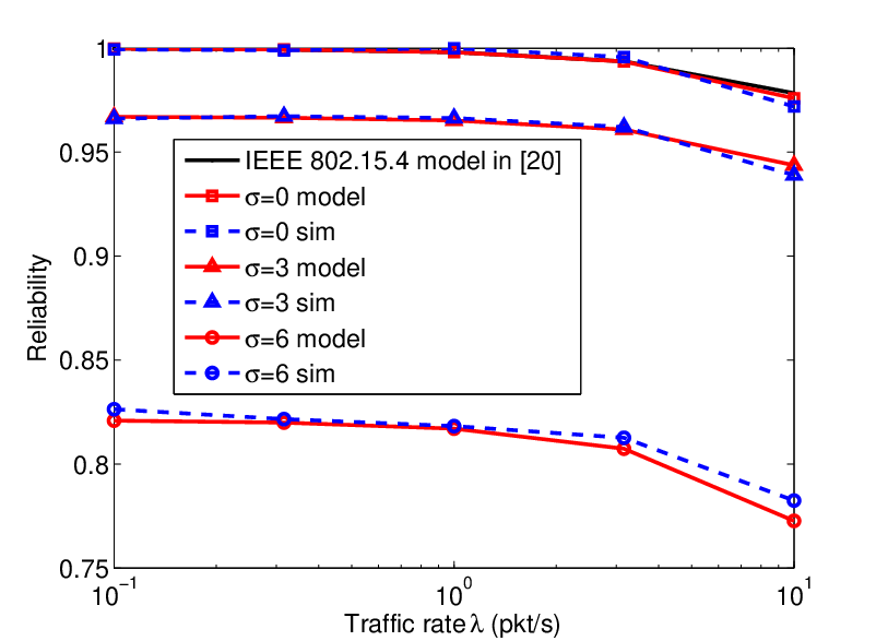
In Fig. 2, we report the average reliability over all links by varying the node traffic rate . The results are shown for different values of the spread and in the absence of multi-path (). The model is compared with the results obtained by using the model in [20], which was developed in the absence of a channel model. There is a good matching between the simulations and the analytical expression (24). The reliability decreases as the traffic increases. Indeed, an increase of the traffic generates an increase of the contention level at MAC layer. Our model is close to the ideal case in [20] in the absence of stochastic fluctuation of the channel (=0). The small gap is due to the presence of thresholds for channel sensing and outage, which reduce the reliability due to possible failures in the CCA mechanism. However, a remarkable aspect is that the impact of shadow fading is more relevant than variations in the traffic. Therefore, a prediction based only on Markov chain analysis of the MAC without including the channel behavior, as typically done in the previous literature, is largely inaccurate to capture the performance of IEEE 802.15.4 wireless networks, especially at larger shadowing spreads.
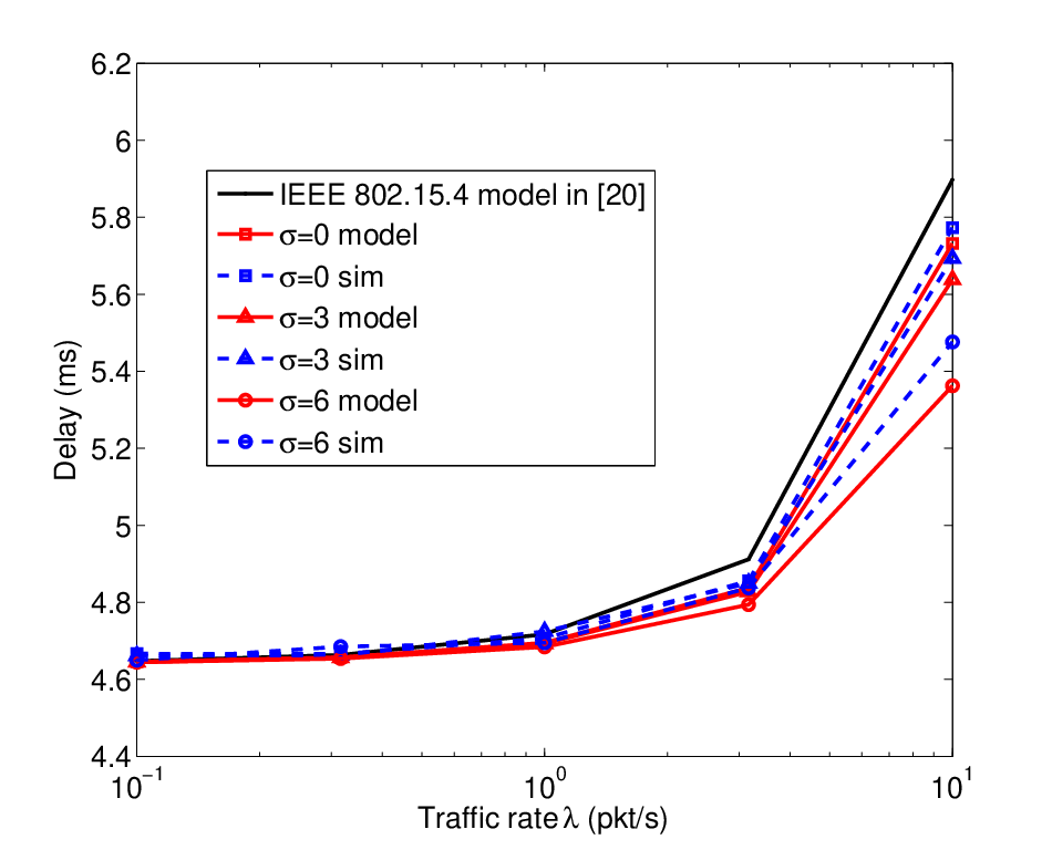
In Fig. 3, the average delay over all links is reported. Also in this case simulation results follow quite well results obtained from the model as given by Eq. (25). The delay in our model with =0 is lower than the delay evaluated in the model in [20] due to the effects of thresholds for channel sensing and outage, which reduce the reliability due to possible failures in the CCA mechanism. An increase of traffic leads to an increase of the average delay due to the larger number of channel contentions and consequently an increase in the number of backoffs. The spread of shadowing components does not impact on the delay significantly, particularly for low traffic, because lost packets due to fading are not accounted for in the delay computation. When the traffic increases, we note that fading is actually beneficial for the delay. In fact, the delay of successfully received packets reduces by increasing . This is because the occurrence of a deep fading reduces the probability of successful transmission. However, since this holds for all nodes, the average number of contending nodes for the CCA may reduce, thus reducing the average delay of successfully received packets. It is not possible to capture this network behavior by using separate models of the IEEE 802.15.4 MAC and physical layers as in the previous literature, since this effect clearly depends on a cross-layer interaction.
In Fig. 4, the average power consumption over all links is presented and compared with the analytical expression in Eq. (30). The number of packet transmissions and ACK receptions is the major source of energy expenditure in the network. Therefore, an increase of the traffic leads to an increase of the power consumption, while performance are marginally affected by the spread of the fading. However, the power consumption is slightly reduced when the spread is , due to the smaller number of received ACKs. Note that no power control policy is implemented.
In Fig. 5, the average reliability is reported as a function of the radius for different values of the spread . Again, analytical results obtained through Eq. (24) are in good agreement with those provided by simulations. For the ideal channel case (i.e., ) the size of the network does not affect the reliability in the range m. For , the performance degrades significantly as the radius increases. An intermediate behavior is obtained for , where the reliability is comparable to the ideal channel case for short links, but it reduces drastically for m. The effect is the combination of an increase of the outage probability with the radius (due to the path loss component) and hidden terminals that are not detected by the CCA.
In Fig. 6, we report the average delay by varying the radius for different values of the spread . The shadowing affects the delay positively and the effect is more significant for larger inter-node distances: in this case the average number of contending nodes for the free channel assessment reduces, thus the busy channel probability reduces, which in turn decreases the average delay of successfully received packets.
In Fig. 7, the average power consumption by varying is presented. We notice a similar behavior as for the delay. The power consumption reduces with the fading and the increasing size of the network. Nodes spend less time in the backoff and channel sensing procedure due to reduced number of contending nodes and the number of ACKs.
Fig. 8 shows the average reliability as a function of the shadowing spread . The results are plotted for different values of the carrier sensing threshold . The reliability decreases when the threshold become larger. The impact of the variation of the threshold is maximum for , and the gap reduces when the spread increases. In Fig. 9, the average delay is plotted as a function of the spread . Depending on the threshold , the delay shows a different behavior when increasing : it increases for dBm and it decreases for dBm, and dBm. As we discussed above, the spread may reduce the delay under some circumstances. However, when the threshold is large, the average number of contenders is less influenced by the fading and does not decrease significantly, while the busy channel probability becomes dominant and the number of backoffs increases, so that the delay increases as well. Fig. 10 reports the average power consumption by varying the spread . The power consumption reduces by increasing the threshold as a consequence of the smaller number of ACK transmissions, although a maximum consumption is observed for low values of the spread.
In Fig. 11, we plot the average reliability as a function of the spread for different values of the outage threshold . The threshold does not affect the performance noticeably for , while the gap in the reliability increases with . Note that for a high threshold the reliability tends to increase with as long as is small or moderate, and it decreases for large spreads. In our setup, a maximum in the reliability is obtained for .
In Fig. 12, we report the combined effects of shadow fading and multi-path fading on the reliability. We show the reliability as a function of the spread of the shadow fading for different values of the Nakagami parameter . We recall that corresponds to Rayleigh fading. There is a good match between the simulations and the analytical model (24). The effect of the multi-path is a further degradation of the reliability. However, the impact reduces as the Nakagami parameter increases and the fading becomes less severe. In fact, for , the effect of multi-path becomes negligible. Furthermore, the multi-path fading and the composite channel evidences the presence of the maximum at in the plot of reliability.
V-B Multi-hop Linear Topologies
In this set of performance results, we consider the multi-hop linear topology in Fig. 1b). The number of nodes is , with the same MAC and physical layer parameters as in the single-hop case. We validate our model and study the performance of the network as a function of the hop distance in the range m, and the spread of the shadow fading in the range . We show results for each hop, and for different values of the carrier sensing threshold dBm, and outage threshold dB.
In Fig. 13, the end-to-end reliability is reported from each node to the destination node for different values of the spread . The analytical model follows well the simulation results. The end-to-end reliability decreases with the number of hops. This effect is more evident in the presence of shadowing. Fig. 14 shows the end-to-end reliability from the farthest node to the destination by varying the distance between every two adjacent nodes for different values of the spread . The reliability is very sensitive to an increase of the hop distance. In Fig. 15, we show the end-to-end reliability by varying the spread of the shadow fading. Results are shown for different values of the carrier sensing threshold . In Fig. 16, we plot the end-to-end reliability for different values of . Similar considerations as for the single-hop case applies here. However, for the linear topology, the reduction of the carrier sensing range from dBm to dBm influences less the reliability since hidden nodes are often out of range of the receiver, therefore the channel detection failure may not lead to collisions.
V-C Multi-hop Topologies with Multiple End-devices



We consider the multi-hop topology in Fig. 1c). We use the same MAC and physical layer parameters as in the single-hop case. We consider the end-to-end reliability as the routing metric and study the performance of the network as a function of the traffic , , in the range pkt/s, the spread of the shadow fading in the range . Moreover, we show results for different values of the Nakagami parameter and threshold dB.
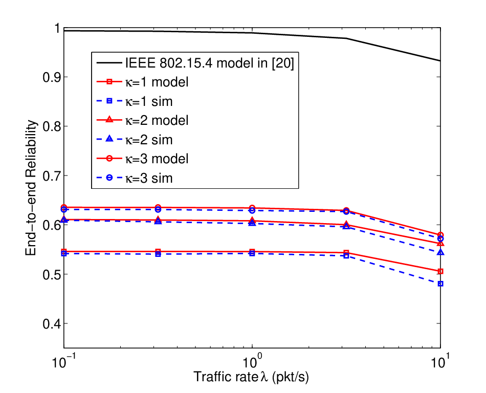
In Fig. 17, we report the average end-to-end reliability over all the end-devices by varying the node traffic rate. The results are shown for different values of Nakagami parameter with the shadowing spread set to . The impact of the Nakagami parameter seems more prominent than variation of the traffic. Fig. 18 shows the end-to-end reliability by varying the spread for different values of . Differently to the other topologies, a variation of the outage threshold has a strong impact on the reliability also for small to moderate shadowing spread. In fact, due to the variable distance between each source-destination pair, the fading and the outage probabilities affect the network noticeably. This effect is well predicted by the developed analytical model.
VI Conclusions
In this paper, we proposed an integrated cross-layer model of the MAC and physical layers for unslotted IEEE 802.15.4 networks, by considering explicit effects of multi-path shadow fading channels and the presence of interferers. We studied the impact of fading statistics on the MAC performance in terms of reliability, delay, and power consumption, by varying traffic rates, inter-nodes distances, carrier sensing range, and SINR threshold. We observed that the severity of the fading and the physical layer thresholds have significant and complex effects on all performance indicators, and the effects are well predicted by the new model. In particular, the fading has a relevant negative impact on the reliability. The effect is more evident as traffic and distance between nodes increase. However, depending on the carrier sensing and SINR thresholds, our model shows that a fading with small spread can improve the reliability with respect to the ideal case. The delay for successfully received packets and the power consumption are instead positively affected by the fading and the performance can be optimized by properly tuning the thresholds.
We believe that the design of future WSN-based systems can greatly benefit from the results presented in this paper. As a future work, a tradeoff between reliability, delay, and power consumption can be exploited by proper tuning of routing, MAC, and physical layer parameters. Various routing metrics can be analyzed, and the model extended to multiple sinks.
References
- [1] IEEE 802.15.4 Wireless Medium Access Control (MAC) and Physical Layer (PHY) Specifications for Low-Rate Wireless Personal Area Networks (WPANs), 2006, http://www.ieee802.org/15/pub/TG4.html.
- [2] A. Willig, “Recent and emerging topics in wireless industrial communication,” IEEE Transactions on Industrial Informatics, vol. 4, no. 2, pp. 102–124, 2008.
- [3] J. Zheng and M. L. Lee, “Will IEEE 802.15.4 make ubiquitous networking a reality?: A discussion on a potential low power, low bit rate standard,” IEEE Communications Magazine, vol. 42, no. 6, pp. 140–146, 2004.
- [4] J. Mis̆ić, S. Shaf, and V. Mis̆ić, “Performance of a beacon enabled IEEE 802.15.4 cluster with downlink and uplink traffic,” IEEE Transactions Parallel and Distributed Systems, vol. 17, no. 4, pp. 361–376, 2006.
- [5] S. Pollin, M. Ergen, S. C. Ergen, B. Bougard, L. Perre, I. Moerman, A. Bahai, P. Varaiya, and F. Catthoor, “Performance analysis of slotted carrier sense IEEE 802.15.4 medium access layer,” IEEE Transactions on Wireless Communication, vol. 7, no. 9, pp. 3359–3371, 2008.
- [6] P. Park, P. Di Marco, P. Soldati, C. Fischione, and K. H. Johansson, “A generalized Markov chain model for effective analysis of slotted IEEE 802.15.4,” in Proceedings of the 6th IEEE International Conference on Mobile Ad-hoc and Sensor Systems MASS, 2009.
- [7] C. Y. Jung, H. Y. Hwang, D. K. Sung, and G. U. Hwang, “Enhanced Markov chain model and throughput analysis of the slotted CSMA/CA for IEEE 802.15.4 under unsaturated traffic conditions,” IEEE Transactions on Vehicular Technology, vol. 58, no. 1, pp. 473–478, 2009.
- [8] J. He, Z. Tang, H.-H. Chen, and Q. Zhang, “An accurate and scalable analytical model for IEEE 802.15.4 slotted CSMA/CA networks,” IEEE Transactions on Wireless Communications, vol. 8, no. 1, pp. 440–448, 2009.
- [9] C. Buratti, “Performance analysis of IEEE 802.15.4 beacon-enabled mode,” IEEE Transactions on Vehicular Technology, vol. 59, no. 4, pp. 2031–2045, 2010.
- [10] A. Faridi, M. Palattella, A. Lozano, M. Dohler, G. Boggia, L. Grieco, and P. Camarda, “Comprehensive evaluation of the IEEE 802.15.4 MAC layer performance with retransmissions,” IEEE Transactions on Vehicular Technology, vol. 59, no. 8, pp. 3917–3932, 2010.
- [11] G. Bianchi, “Performance analysis of the IEEE 802.11 distributed coordination function,” IEEE Journal on Selected Areas in Communications, vol. 18, no. 3, pp. 535–547, 2000.
- [12] M.-H. Zayani, V. Gauthier, and D. Zeghlache, “A joint model for IEEE 802.15.4 physical and medium access control layers,” in Proceedings of the 7th International Wireless Communications and Mobile Computing Conference IWCMC, 2011.
- [13] X. Yang and N. Vaidya, “On physical carrier sensing in wireless ad hoc networks,” in Proceedings of the 24th IEEE International Conference on Computer Communications INFOCOM, 2005.
- [14] F. Daneshgaran, M. Laddomada, F. Mesiti, and M. Mondin, “Unsaturated throughput analysis of IEEE 802.11 in presence of non ideal transmission channel and capture effects,” IEEE Transactions on Wireless Communications, vol. 7, no. 4, pp. 1276–1286, 2008.
- [15] D. Hoang and R. Iltis, “Performance evaluation of multi-hop csma/ca networks in fading environments,” IEEE Transactions on Communications, vol. 56, no. 1, pp. 112–125, 2008.
- [16] E. J. Leonardo and M. D. Yacoub, “Exact formulations for the throughput of IEEE 802.11 DCF in Hoyt, Rice, and Nakagami-m fading channels,” IEEE Transactions on Wireless Communications, vol. 12, no. 5, pp. 2261–2271, 2013.
- [17] G. Sutton, R. Liu, and I. Collings, “Modelling IEEE 802.11 DCF heterogeneous networks with Rayleigh fading and capture,” IEEE Transactions on Communications, vol. PP, no. 99, pp. 1–13, 2013.
- [18] C. Gezer, C. Buratti, and R. Verdone, “Capture effect in IEEE 802.15.4 networks: modelling and experimentation,” in Proceedings of the 5th IEEE International Symposium on Wireless Pervasive Computing ISWPC, 2010.
- [19] A. Iyer, C. Rosenberg, and A. Karnik, “What is the right model for wireless channel interference?” IEEE Transactions on Wireless Communications, vol. 8, no. 5, pp. 2662–2671, 2009.
- [20] P. Di Marco, P. Park, C. Fischione, and K. H. Johansson, “Analytical modeling of multi-hop IEEE 802.15.4 networks,” IEEE Transactions on Vehicular Technology, vol. 61, no. 7, pp. 3191–3208, 2012.
- [21] M. Pratesi, F. Santucci, and F. Graziosi, “Generalized moment matching for the linear combination of lognormal rvs: application to outage analysis in wireless systems,” IEEE Transactions on Wireless Communications, vol. 5, no. 5, pp. 1122 –1132, 2006.
- [22] C. Fischione, F. Graziosi, and F. Santucci, “Approximation for a sum of on-off log-normal processes with wireless applications,” IEEE Transactions on Communications, vol. 55, no. 9, pp. 1822 – 1822, 2007.
- [23] D. P. Bertsekas and J. N. Tsitsiklis, Parallel and Distributed Computation: Numerical Methods. Athena Scientific, 1997.
- [24] The ns2 network simulator, 2011. [Online]. Available: http://www.isi.edu/nsnam/ns/