Avalanches and dimensional reduction breakdown in the critical behavior of disordered systems
Abstract
We investigate the connection between a formal property of the critical behavior of several systems in the presence of quenched disorder, known as “dimensional reduction”, and the presence in the same systems at zero temperature of collective events known as “avalanches”. Avalanches generically produce nonanalyticities in the functional dependence of the cumulants of the renormalized disorder. We show that this leads to a breakdown of the dimensional reduction predictions if and only if the fractal dimension characterizing the scaling properties of the avalanches is exactly equal to the difference between the dimension of space and the scaling dimension of the primary field, e.g. the magnetization in a random field model. This is proven by combining scaling theory and functional renormalization group. We therefore clarify the puzzle of why dimensional reduction remains valid in random field systems above a nontrivial dimension (but fails below), always applies to the statistics of branched polymer and is always wrong in elastic models of interfaces in a random environment.
In the theory of disordered systems, “dimensional reduction” is the property shared by some models that the long-distance physics in the presence of quenched disorder in some spatial dimension is the same as that of the pure model with no disorder in a reduced spatial dimension, . In the known examples where it has been found through perturbation theory, i.e. the random field Ising model (RFIM) [1, 2, 3], elastic manifolds in a random environment [4], the random field and random anisotropy O(N) models [1, 2, 3, 6] and the statistics of dilute branched polymers11 1 We include the branched polymer problem in the list of disordered systems by an abuse of language. Indeed, there is no quenched disorder in this case but the equivalence comes from the limit which is common to the field-theoretical description of self-avoiding polymer chains and to the replica theory of disordered systems. The dimensional reduction then leads to the Yang-Lee edge singularity in dimension . See Ref. [7]., it entails two conditions: (1) that the long-distance physics is controlled by a zero-temperature fixed point, so that it can be equally described from the solution(s) of a stochastic field equation at zero temperature, and (2) that an underlying supersymmetry (involving rotational invariance in superspace) emerges in the field-theoretical treatment of the stochastic equation [5, 7, 8]. Dimensional reduction however is known to be wrong in some of the above models, the random field and random anisotropy models in low enough dimension (a rigorous proof exists for the RFIM in and [9, 10]) and the elastic manifold in a random environment [4]. On the other hand, it is proven to be right for the branched polymer case in all dimensions below the upper critical one [11, 12].
We have recently shown that the breakdown of dimensional reduction and the spontaneous breaking of the underlying supersymmetry take place below a nontrivial critical dimension22 2 Actually, the two phenomena take place at two very close but distinct critical dimensions and , with ; the former represents the point at which supersymmetry is spontaneously broken along the flow and the dimensional-reduction fixed point vanishes and the latter is where the dimensional-reduction fixed point becomes unstable to a nonanalytic perturbation. For the RFIM, the two are numerically almost indistinguishable and for the RFO(N)M one finds and when approaching [G. Tarjus, M. Baczyk, and M. Tissier, in preparation (2012)]. in the random-field Ising, and more generally O(N), model: this dimension is close to for the Ising () version and decreases continuously as increases until it reaches when approaches (the upper critical dimension is equal to for random field systems) [13, 14, 15]. Describing this phenomenon requires a renormalization group (RG) approach that is functional, as the origin of the dimensional reduction breakdown is the appearance of a nonanalytic dependence of the renormalized cumulants of the random field (a linear “cusp”) in the dimensionless fields, and nonperturbative, as it takes place away from regimes where some form of perturbation analysis is possible (except for the O(N) model when is close to the lower critical dimension of 4 [13, 15]). A similar conclusion was previously reached for the case of an elastic manifold in a random environment, but in this model the dimensional reduction predictions fail for all dimensions at and below the upper critical dimension (here equal to ) and can be already assessed through a functional but perturbative RG [16, 17, 18, 19]. What is the physical mechanism behind these seemingly formal results?
The existence of a cusp in the cumulants of the renormalized disorder can be assigned to the presence of collective events known as “avalanches”. In any typical sample of a disordered model, the ground state, which is the relevant configuration that describes the equilibrium properties of the system at zero temperature, abruptly changes for specific values of the external source; the location of these abrupt changes are sample-dependent and the configurational change between two ground states is precisely an avalanche [20, 21, 22, 23, 24, 25, 26]. (The latter is sometimes called a ‘‘static’’ avalanche33 3 In the context of elastic interfaces in a disordered environment, the static avalanches are also called “shocks” by analogy with the behavior found in the Burgers equation [27, 28]..) The same phenomenon is observed, still at zero temperature, when the system is driven by the external source without being allowed to equilibrate. The corresponding “dynamic” avalanches then take place out of equilibrium, between two metastable states of the system [29, 30, 31, 32, 33, 25].
However, the fact that abrupt changes corresponding to discontinuous variations of the magnetization (to use the language of magnetic systems) are found at zero temperature should come as no surprise. In disordered systems, this can take place even in noninteracting zero-dimensional models. Consider for instance a (single point) theory with parameters such that the potential has two minima and couple the field to a random source and a controllable source . Then, according to the value of , the ground state of the system will switch from the vicinity of one minimum to that of the other one with a jump in the magnetization (the field ) when . This jump corresponds to an avalanche, albeit a zero-dimensional one. As will be illustrated in more detail below, these avalanches do generate a cusp in the cumulants of the effective random field (see Fig. 1). However, avalanches, and the resulting nonanalyticities in renormalized disorder cumulants, affect the long-distance physics of a -dimensional disordered model and play a role in the failure of dimensional reduction only if they are of collective origin and occur on sufficiently large scales.
From the above discussion we conclude that in disordered systems, (i) the physics of dimensional reduction and its breakdown is associated with an effective zero-temperature theory, (ii) avalanches corresponding to discontinuous jumps of the magnetization and more generally of the field configuration are the rule rather than the exception at zero temperature and (iii) the dimensional-reduction breakdown results from the presence of avalanches that must be collective enough to influence the long-distance properties of the model. The central question is then: Under which conditions does this happen? We show that dimensional reduction remains valid when the exponent that characterizes the scaling behavior of the largest typical avalanches at criticality is strictly less than the difference between the spatial dimension and the scaling dimension of the field near the relevant zero-temperature fixed point: . This condition is satisfied for the RFIM at and close to the upper critical dimension and for branched polymers at and around the upper critical dimension and below (at least). On the other hand, dimensional reduction breakdown takes place when is equal to 44 4 The condition leads to unphysical results, as discussed further down. This is found for elastic manifolds in a random environment at and near the upper critical dimension as well as for the RFIM below a critical dimension close to . This clarifies the intriguing result of why dimensional reduction fails below a nontrivial dimension for the RFIM, is always broken for random elastic manifolds, but applies to the branched-polymer problem.
Avalanches and their consequences on the cumulants of the renormalized disorder. Take a disordered system at zero temperature in which avalanches, representing discontinuous changes of the relevant configuration of the system under a variation of an external source, are present. We use the language of magnetic systems and characterize configurations by the local magnetization. All considerations, however, equally well apply to configurations described by a continuous field, in or out of equilibrium, and to nonmagnetic systems, e.g. to the displacement of an interface in a random medium [20, 21, 29, 35] or to the appropriate density field describing the universal properties of dilute branched polymers. We focus on situations in which the field under study (the “magnetization”) is the local order parameter and is linearly coupled to the external source, but one should keep in mind that avalanches could also be triggered by changing for instance the strength of the disorder [36, 37] at zero temperature and that avalanches may involve a field that is not the local order parameter (e.g., the magnetization in a spin glass [38, 39, 40]).
Consider for simplicity an external source that is uniform in space. The avalanches can then be characterized by their size (the overall change in the total magnetization55 5 In principle, the size of an avalanche, if defined in terms of the total number of spins that flip in an Ising model or of an equivalent geometric quantity in a field theory, could be different from the associated change in magnetization. This is for instance what is predicted for spin glasses by the droplet theory [55]. However, for the systems under study, one expects and proves in several cases that the size and the magnetization are essentially the same and scale in the same way with the (linear) spatial extent of the avalanche.) whose distribution is described by a density , such that is the (disorder averaged) number of avalanches of size between and when the source is between and . The magnetization is the spatial average of the local order parameter field for a given sample characterized by the disorder realization . Its change between two values of the external source and is the sum of two contributions: a first one comes from the smooth changes in the ground state (in equilibrium) or in the metastable state (out of equilibrium) and another one comes from the avalanches that take place between and (with ). As a consequence, the moments of the difference , which is a random variable, are given by
| (1) | ||||
where the first term is due to avalanches taking place at the same value of the external source and the second term, denoted by , includes the contributions involving the smooth variation of the magnetization or distinct avalanches. is a microscopic lower cutoff on the size of the avalanches, is the sample volume, and the overline denotes the average over the quenched disorder.
For even moments, due to the symmetry in the exchange of and , the first term in Eq. (1) gives rise to a linear cusp when :
| (2) | ||||
[The other term in Eq. (1) is regular or at least less singular than the first one and is therefore a .]
It is easily realized that the th moment is obtained by considering disorder averages over copies of the same sample, with each copy coupled to a distinct external source , . The first moment is the change in the average magnetization of the system and the th cumulant (which is the connected piece of the th moment) is then related to Green’s functions at zero momentum of a -copy system in which each copy is characterized by a distinct source. For example, the relevant 2-point Green’s function, given by , is an extension to general sources of what is usually called the “disconnected” 2-point correlation function in the theory of disordered systems. One-particle irreducible (1PI) correlation functions (or proper vertices) [41] associated with the above Green’s functions can be introduced along the same lines66 6 For the equilibrium case, this is simply done through a Legendre transformation that allows one to go from the generating functional depending on the external sources to the one depending on the local magnetization (the Gibbs free-energy in the language of magnetic systems) or the classical field (the effective action in the language of quantum field theory). This can be generalized to the out-of-equilibrium case but requires the introduction of auxiliary fields.. From Eq. (2), one immediately derives that, for instance, the -point Green’s function has a nonanalytic dependence as , with the amplitude of the cusp related to the second moment of the avalanches:
| (3) |
This can be transposed to the associated 1PI vertices and can generalized to higher orders as well77 7 We have discussed the case where the relevant variable or field involved in the avalanches has a single component. Cusps and avalanches are also present in the case of multi-component fields (see e.g., Ref. [42]). However, as the analysis is more complex, we mostly restrict ourselves here to the consideration of systems with a single-component field..
(a)
(b) 
(c)
The above arguments show that avalanches induce a linear cusp in the functional dependence of the correlation functions describing the cumulants of the effective or renormalized disorder at . This is always true even when the avalanches take place on a restricted scale, away from any critical conditions (see Fig. 1 for an illustration). However, we are interested in the long-distance behavior of disordered systems. We therefore study the situation in which avalanches occur on all scales, as found for instance in the RFIM at the equilibrium or out-of-equilibrium critical point, in the rough phase of an elastic manifold pinned by a random medium or at its depinning transition, etc.
Consider a -dimensional system of linear size at zero temperature. At large scale, when the correlation length and the extent of the largest typical avalanches have reached the system size, one expects that the (normalized) probability density of having an avalanche of size (see footnote 5) can be written in the following scaling form [34, 33, 25, 26]:
| (4) |
where is the size the largest typical ‘‘critical’’ avalanches in the finite system88 8 In a finite-size system it may be important to appropriately sort out the various classes of large, system-spanning avalanches: the relevant ones for the critical scaling have been called “spanning critical” in the context of the out-of-equilibrium RFIM [33] and is then the associated exponent.; acts as a cutoff for the scaling function that decays exponentially for . Critical conditions correspond to (for the RFIM at equilibrium one has due to the symmetry and for the random manifolds there is no condition on as the whole phase is critical). The avalanche size distribution is normalized so that and the moments of the normalized avalanche size distribution are then defined as . When , which is usually found (for instance, the mean-field value for is equal to in all models), the normalization factor is dominated by the small avalanches whereas all moments with are dominated by the largest typical avalanches and behave as when .
We keep using the language of magnetic systems and let denote the magnetization of a given sample of linear size . (Here and below, we explicitly indicate the dependence on the system size ; this makes the expressions somewhat clumsy but will be helpful later on to make the connection with the results of the functional RG.) We are primarily interested in the moments of the random variable . The density of avalanches [see Eq. (1)] is related to the normalized probability density by an overall and dependent factor: . As discussed before in connection to Eq. (1), the first moment of contains a contribution from the smooth change of the magnetization and one from the avalanches. The so-called “connected” susceptibility , which is the standard magnetic susceptibility divided by the temperature in order to have a proper zero-temperature limit and which is obtained by deriving with respect to , can then be expressed as
| (5) |
Under critical conditions, goes as . By further making the natural assumption that the contribution from the avalanches is of the order or larger than the smooth one and by using Eqs. (4,5) as well as the fact that the first moment of the avalanches is dominated by large avalanches, one then obtains that
| (6) |
As a result, Eq. (2) can be rewritten as
| (7) | ||||
and the linear cusp in the 2-point Green’s function at zero momentum when [see eq. (3)] is found as
| (8) | ||||
up to a . The amplitude of the cusp therefore diverges as the size of the system diverges. (One should however keep in mind that the whole function itself diverges as at criticality.) The above result generalizes to higher-order Green’s functions through their relation to the cumulants of the magnetization.
From Eq. (8), it is easily derived that the associated 1PI correlation function , which is the second cumulant of the renormalized disorder, also has a cusp in as . After introducing and , where and corresponds to the value of the average magnetization at criticality, and using the relation between Green’s functions and 1PI functions (see ref. [41] and footnote 6) as well as when , we obtain, up to a ,
| (9) | ||||
where we have also used that . Again, the above expression can be generalized to higher-order cumulants of the renormalized disorder, which all display a cusp in their functional dependence with an amplitude that is system-size dependent at criticality.
Functional RG and dimensional reduction breakdown. As already stressed, the functional RG is a powerful and necessary framework to describe the critical behavior of the disordered systems of interest. Within such an approach, which is a version of Wilson’s continuous RG [43, 44, 45, 46], the fluctuations are progressively taken into account by introducing an infrared cutoff that enforces the decoupling of the low- and high-momentum modes at a running scale . For , all fluctuations are included and the exact theory is recovered. One ends up with flow equations for the moments of the renormalized disorder that describe the evolution of these moments as one decreases the infrared scale . For instance, an equation is obtained for the second cumulant of the renormalized random field or random force [16, 17, 18, 19, 13, 14, 15], which is the quantity already considered in the previous sections, with the field and the infrared scale playing here the same role as the local magnetization and the inverse system size , respectively. (This RG equation for is in general part of a hierarchy of coupled flow equations.)
In order to reach the fixed point that controls the long-distance behavior under study, one must introduce scaling dimensions and convert the quantities appearing in the RG flow equations from “dimensionful” to “dimensionless”. For the cases of interest where on the one hand avalanches are present and on the other hand dimensional reduction is found in standard perturbation theory, we have stressed that the fixed point is at zero temperature. Temperature is then a dangerously irrelevant variable, and an associated exponent is introduced through an appropriate definition of a renormalized temperature [47, 48, 16, 17, 18, 19, 13, 14, 15]: . Near the zero-temperature fixed point, the dimension of the field is modified from its standard value of , with the anomalous dimension, by a term involving the temperature exponent:
| (10) |
where we have also introduced the additional anomalous dimension through the relation . Similarly, the second cumulant of the renormalized random field or force has the scaling dimension of a -point 1PI vertex, , modified by the temperature exponent, i.e. ; it can be put in dimensionless form as
| (11) |
where is the dimensionless field (see also SI appendix).
Dimensional reduction corresponds to , which implies , and to all other exponents equal to their value in the system without disorder in dimension . The main outcome of the functional RG studies is that breakdown of dimensional reduction is related to the presence of a cusp in the functional dependence of the dimensionless second cumulant of the renormalized random field or force, , in the vicinity of the zero-temperature fixed point [16, 17, 18, 19, 13, 14, 15]. More concretely, after introducing and , the “cuspy” behavior that changes the critical exponents from their dimensional reduction prediction is of the form
| (12) |
when , with ; the star indicates the fixed-point value at . As a result of a nonzero , the exponent takes a nontrivial -dependent value and and differ from the dimensional reduction values, with .
The connection between the quantities computed through the functional RG and those discussed in the previous sections can be made by associating the infrared cutoff with the inverse of the linear extent of the system, i.e. . Eq. (9) can then be expressed in a dimensionless form by dividing the cumulant and the magnetization by their scaling dimensions and , respectively. We immediately obtain that the amplitude of the linear cusp in dimensionless form scales as with
| (13) |
which can also be rewritten as . By comparison with Eq. (12), one therefore finds that the cusp persists in the dimensionless quantities when , i.e. at the fixed point, if and only if . If , the cusp is only subdominant and does not affect the leading critical behavior and the associated exponents. (Note that the condition is not compatible with the result of the functional RG studies, in which proper renormalized theories have always been found with no stronger nonanalyticities than the linear cusp.)
We conclude from the above derivation that dimensional reduction breaks down due to avalanches if the fractal dimension of the largest typical “critical” avalanches satisfies the condition
| (14) |
On the other hand, dimensional reduction remains valid if
| (15) |
despite the presence of the avalanches and of a cusp in the dimensionful cumulants of the effective disorder at zero temperature. In the latter case, the difference can be reinterpreted and computed in the functional RG. Indeed when perturbing the ‘‘cuspless’’ fixed-point value99 9 Weaker nonanalyticities, i.e. subcusps, could still be present but do not affect dimensional reduction [13, 14]). of the dimensionless cumulant with a function that itself displays a linear cusp, the amplitude of the cuspy perturbation should go to zero as in such a way that
| (16) |
with and when . Information on the fractal dimension of the largest typical avalanches at criticality can then be obtained from an investigation of the irrelevant directions associated with nonanalytic eigenfunctions around the fixed point. This is what we have done by solving the nonperturbative functional RG equations derived in Ref. [15] for a function of the form given in Eq. (16) (see SI appendix).
Results and discussion. We are now in a position to discuss the consequences of Eqs. (14) and (15) for several disordered systems in which dimensional reduction is predicted by standard perturbation theory.
Consider first the mean-field limit. Avalanches are present at and the distribution of the avalanche sizes at criticality can be described by the scaling expression in Eq. (4). The exponents and can be easily derived for fully connected models. This was first done by Dahmen and Sethna [34] for the out-of-equilibrium behavior of the slowly driven RFIM at zero temperature, but can be generalized to other models as well. (As usual, the mean-field exponents are expected to be “super-universal”.) The values of the avalanche exponents are and . These values have also been recovered by Le Doussal and Wiese [35] from a field-theoretical treatment of elastic manifolds in a random environment. What conclusion can then be drawn about the influence of the avalanches on the long-distance physics? At the upper critical dimension at which the exponents take their mean-field values, the anomalous dimension so that . The conditions in Eqs. (14) and (15) simply amount to comparing and . For random field and random anisotropy models (we include here models with -component fields which we expect to behave in a similar manner as that of the single-component one), the upper critical dimension is so that dimensional reduction should apply. The same is true for the statistics of dilute branched polymer for which the upper critical dimension is [49]. On the other hand, for interfaces in a disordered environment, the upper critical dimension is : a failure of dimensional reduction is then expected, possibly only in logarithmic corrections at but more severe as one lowers the dimension.
As one decreases the dimension from the upper critical one, there must be a nonzero range of dimensions for which the dimensional reduction predictions correctly describe the critical behavior of the random field, random anisotropy and branched polymer models, but likely not that of the random manifold one. Actually, the latter model has been studied in great detail by the perturbative functional RG in [21, 29, 35]. It was found that the dimension characterizing the cutoff on large avalanches in the presence of a finite-size or infrared cutoff on the system is equal to , where is the exponent describing the roughness of the interface (for a single-component displacement field). As the dimension of the field is itself equal to ( is formally equal to ), it follows that the equality is always verified and that dimension reduction never applies, as indeed found by direct computation of the critical exponents within the functional RG or in computer simulations. This conclusion is valid for the pinned phase, in equilibrium, and for the depinning threshold in the driven case.
For the RFIM at equilibrium, we have shown through a nonperturbative functional RG that dimensional reduction breaks down below a nontrivial critical dimension (see Refs. [14, 15] and footnote 2). According to the above conditions, the avalanche exponent should then be equal to below and to , where is the eigenvalue associated with the irrelevant cuspy directions around the cuspless fixed point (see preceding section and SI appendix), above . In Fig. 2, we plot the theoretical prediction for based on the above relations and the computation of and from the solution of the flow equations previously derived in our nonperturbative functional RG approach of the RFIM [15] (see also footnote 2). The prediction is confirmed at the upper (see above) and lower critical dimensions. For the latter, , one indeed expects the avalanches to be compact even at criticality and their fractal dimension therefore to be equal to the spatial dimension, (see also Ref. [31]). As the dimension of the field is equal to zero, (and ), the equality in Eq. (14) is satisfied. (Note that the results at the lower and upper critical dimensions apply to both the equilibrium and out-of-equilibrium critical behavior of the RFIM1010 10 It has also been suggested that the critical properties of the RFIM in and out of equilibrium are in the same universality class in all dimensions [31, 33, 25].) Beside this, direct measurements or computations of the avalanche exponent are unfortunately scarce. We therefore suggest that, as done for models of an elastic interface in a disordered environment [20, 21, 29] and for the out-of-equilibrium, metastable behavior of the driven RFIM [31, 32, 33, 25], systematic studies of the avalanches and of the cumulants of the effective (renormalized) disorder would be worthwhile, e.g. in the ground state of the RFIM, and would allow a direct test of the predictions made on the basis of the functional RG.
Finally, for the statistics of dilute branched polymers, so long as dimensional reduction applies, and is negative. In consequence, . As the fractal dimension should also be less than the dimension of space1111 11 This reasoning does not apply to the elastic manifolds in a random environment. In this case, is the dimension of space on which the displacement field describing the location of the manifold is defined. The size of an avalanche, which represents the total amount by which the manifold moves, therefore involves both the “lateral” dimension (by an amount for a system of lateral linear size ) and the change in the displacement field itself ( with the roughness exponent ). In this case, ., one can see that when . From the condition on the scaling of the avalanches in Eq. (15), we therefore obtain that dimensional reduction applies, at least, when and in the vicinity of the upper critical dimension (see above); the existence of an intermediate range of dimensions characterized by dimensional reduction breakdown is highly unlikely. This is of course in agreement with the known results according to which dimensional reduction (to the Lee-Yang edge singularity, or equivalently to the universal repulsive gas singularity, in two fewer dimensions) is always valid in the case of dilute branched polymers [11, 12].

To summarize, we have related the breakdown of “dimensional reduction” to the scaling characteristics of “avalanches”. The former is the formal property according to which the critical behavior in the presence of quenched disorder is the same as that of the clean system in two dimensions less and is found within conventional perturbation theory in models whose long-distance physics is controlled by a zero-temperature fixed point, whereas the latter are large-scale physical events taking place in the relevant configuration of the system (ground state in equilibrium or metastable state out of equilibrium) under the variation of an external source. This provides a solution to the puzzle of why dimensional reduction breaks down in some models and not in others, in some range of dimensions and not for others.
Note finally that at small but nonzero temperature, there are no avalanches and the variation of the relevant configuration of the system under a change of the external source is continuous, except possibly in mean-field models. The nonanalyticities in the functional dependence of the cumulants of the renormalized disorder and of the associated Green’s functions are then rounded in “thermal boundary layers” [51, 52, 53, 14]. In systems at equilibrium, these boundary layers are linked to the presence of low-energy excitations that may also take place on large scales at and near criticality and are described as “droplets” [54, 55]. The relation between droplets and avalanches in disordered systems is by itself a very interesting topic, which however we have not considered here. In any case, this underscores that properties such as dimensional reduction and its breakdown or avalanches crucially depend on the system being at zero temperature or having its critical behavior controlled by a zero-temperature fixed point.
[Nonperturbative functional RG for the RFIM]
We summarize here the main features of the nonperturbative functional RG description of the equilibrium critical behavior of RFIM developed in Refs. [13, 14, 15] as well as its extension to compute the stability of the zero-temperature fixed point against nonanalytic perturbations.
The central quantity is the so-called “effective average action” [46, 56] in which only fluctuations of modes with momentum larger than an infrared cutoff are effectively taken into account. In the language of magnetic systems, is the Gibbs free-energy functional of the local order parameter field obtained after a coarse-graining down to the (momentum) scale . The effective average action obeys an exact RG equation under the variation of the infrared cutoff [46, 56].
In the presence of disorder, the generating or free-energy functionals are sample-dependent, i.e. random, and should therefore be characterized either by their probability distribution or by their cumulants. The latter description is more convenient as it focuses on quantities, cumulants and associated Green’s functions, which are translationally invariant and can be generated through the introduction of copies (or “replicas”) of the original system that are submitted to distinct external sources [13, 15]. The effective average action that generates the cumulants of the renormalized disorder, , then depends on the local order parameter fields associated with the various copies . It satisfies the following exact functional RG flow equation [13, 15]:
| (17) | ||||
where is the matrix formed by the second functional derivatives of with respect to the fields and , where and are infrared cutoff functions that enforce the decoupling of the low- and high-momentum modes at the scale (see below). Note that the formalism can be upgraded to a superfield theory in order to describe the physics directly at zero temperature (i.e., at equilibrium, the ground-state properties) [15]: this allows one to make the underlying supersymmetry of the model explicit [5] and to consider features associated with spontaneous or explicit breaking of the latter [15].
From Eq. (17), one can derive a hierarchy of coupled RG flow equations for the cumulants of the renormalized disorder, , , etc, that are obtained from through an expansion in increasing number of unrestricted sums over copies:
| (18) |
At the microscopic scale, say , the effective average action reduces to the “bare” action (or effective hamiltonian) of the multy-copy system
| (19) | ||||
which generates the cumulants of the renormalized disorder at the mean-field level ( is the bare variance of the random field that is taken with a Gaussian distribution of zero mean). At the end of the flow, when , all fluctuations are incorporated and one recovers the effective action which is the generating functional of the cumulants of the renormalized disorder and corresponds in the language of magnetic systems to the exact Gibbs free-energy functional of the multi-copy system.
The detour via the superfield formalism provides a nonperturbative approximation scheme for the exact RG equation, Eq. (17), and a relation between the cutoff functions and which, both, do not explicitly break the underlying supersymmetry at the origin of dimensional reduction. The minimal truncation of that already contains the key features for a nonperturbative study of the long-distance physics of the RFIM is the following:
| (20) |
with three functions , and to be determined. On the other hand, the cutoff functions must satisfy the relation , with the strength of the renormalized random field and the field renormalization constant. Inserting the above ansatz for into Eq. (17) leads to a set of coupled flow equations for the three functions , and (or alternatively its second derivative which is the second cumulant of the renormalized random field at zero momentum discussed in the text). The RG is functional as its central objects are functions instead of coupling constants.
One more step is needed to cast the nonperturbative functional RG flow equations in a form that is suitable for searching for the anticipated zero-temperature fixed points describing the critical behavior of the RFIM. One has to introduce appropriate scaling dimensions. This requires to define a renormalized temperature which should flow to zero as . (This is the precise meaning of a “zero-temperature” fixed point.) Near such a fixed point, one has the following scaling dimensions:
| (21) |
with and related through , as well as
| (22) |
so that the second cumulant of the renormalized random field scales as .
Letting the dimensionless counterparts of be denoted by lower-case letters, , the resulting flow equations can be symbolically written as
| (23) |
where . The beta functions themselves depend on , , and their derivatives [in addition, the running anomalous dimensions and are fixed by the conditions ]. Their expressions are given in Ref. [15].
Fixed points are studied by setting the left-hand sides of the equations in Eq. (23 to zero. The zero-temperature fixed point controlling the critical behavior of the RFIM is once unstable and has been determined in a previous investigation [15]. We found that above a dimension close to , there exists a fixed point with no cusp singularity in the functional dependence of the associated . After introducing and , the dimensionless second cumulant of the renormalized random field can indeed be expanded as
| (24) |
when . It can be shown that the critical behavior then satisfies dimensional reduction: , so that , and the critical exponents are exactly given by those of the pure Ising model in two dimensions less within the nonperturbative approximation that is the counterpart of Eq. (20).
To compute the eigenvalue that characterizes the stability of the above cuspless fixed point with respect to a “cuspy” perturbation, we have considered the vicinity of the fixed point with and set at their fixed-point values and with when . By linearizing the flow equation for around and expanding around it is easy to derive that satisfies the following eigenvalue equation:
| (25) |
where , derivatives of functions of a single argument are denoted by primes and partial derivatives are denoted by superscripts in parentheses; is the square of the dimensionless momentum, is the (dimensionless) cutoff function defined from , and is the (dimensionless) “propagator”, i.e. the -copy, -point Green’s function. Finally, is an operator acting only on the cutoff function (appearing explicitly or through the dimensionless propagator) with . (Choices of appropriate functional forms for are discussed in [15].) In deriving the above equation, we have used the fact that and , which are properties of the dimensional-reduction fixed point.
An equation for the fixed-point function is also derived by inserting the expansion in powers of of [see Eq. (24)] in the corresponding beta function in Eq. (23). The algebra is straightforward but cumbersome and is not worth presenting here. From the knowledge of and , which are obtained from two coupled equations (see Ref. [15]), we first solve the equation for and then use the input to solve Eq. (25). All partial differential equations are numerically integrated on a grid by discretizing the field . The corresponding “cuspless” fixed point only exists above a dimension . Note also that at the upper critical dimension, , one can analytically determine the solution of the above equations: as expected the fixed point is Gaussian and the eigenvalue .
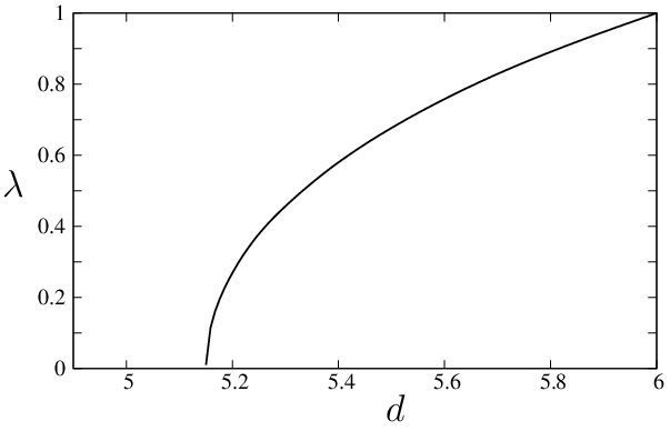
The result for versus spatial dimension is displayed in Fig. 3. Within numerical accuracy, the dimension at which is indistinguishable from , namely (see footnote 2). We have used these values of to construct the curve for the fractal dimension of the largest typical avalanches in Fig. 2.
References
- [1] A. Aharony, Y. Imry, and S. K. Ma, Phys. Rev. Lett. 37, 1364 (1976).
- [2] G. Grinstein, Phys. Rev. Lett. 37, 944 (1976).
- [3] A. P. Young, J. Phys. C 10, L257 (1977).
- [4] K. B. Efetov and A. I. Larkin, Sov. Phys. JETP 45, 1236 (1977).
- [5] G. Parisi and N. Sourlas, Phys. Rev. Lett. 43, 744 (1979).
- [6] D. S. Fisher, Phys. Rev. B 31, 7233 (1985).
- [7] G. Parisi and N. Sourlas, Phys. Rev. Lett. 46, 871 (1981).
- [8] K. J. Wiese, J. Phys.: Condens. Matter 17, S1889 (2005).
- [9] J. Z. Imbrie, Phys. Rev. Lett. 53, 1747 (1984).
- [10] J. Bricmont and A. Kupianen, Phys. Rev. Lett. 59, 1829 (1987).
- [11] D. C. Brydges and J. Z. Imbrie, J. Stat. Phys. 110, 503 (2003); Ann. Math. 158, 1019 (2003).
- [12] J. Cardy, arXiv:condmat/0302495 (2003).
- [13] G. Tarjus and M. Tissier, Phys. Rev. Lett. 93, 267008 (2004); Phys. Rev. B 78, 024203 (2008).
- [14] M. Tissier and G. Tarjus, Phys. Rev. Lett. 96, 087202 (2006); Phys. Rev. B 78, 024204 (2008).
- [15] M. Tissier and G. Tarjus, Phys. Rev. Lett. 107, 041601 (2011); Phys. Rev. B 85, 104202 (2012); ibid, 104203 (2012).
- [16] D. S. Fisher, Phys. Rev. Lett. 56, 1964 (1986).
- [17] O. Narayan and D. S. Fisher, Phys. Rev. B 46, 11520 (1992); Phys. Rev. B 46, 11520 (1993).
- [18] P. Le Doussal, K. J. Wiese, and P. Chauve, Phys. Rev. B 66, 174201 (2002); Phys. Rev. E 69, 026112 (2004).
- [19] P. Le Doussal and K. J. Wiese, Phys. Rev. E 79, 051106 (2009).
- [20] A. A. Middleton, P. Le Doussal and K. J. Wiese, Phys. Rev. Lett. 98, 155701 (2007).
- [21] P. Le Doussal, A. A. Middleton, and K. J. Wiese, Phys. Rev. E 79, 050101 (2009).
- [22] C. Frontera, J. Goicoechea, J. Ortin, and E. Vives, J. Comput. Phys. 160, 117 (2000).
- [23] I. Dukovski and J. Machta, Phys. Rev. B 67, 014413 (2003).
- [24] Y. Wu and J. Machta, Phys. Rev. Lett. 95, 137208 (2005); Phys. Rev. B 74, 064418 (2006).
- [25] Y. Liu and K. A. Dahmen, Phys. Rev. E 76, 031106 (2007); Phys. Rev. E 79, 061124 (2009).
- [26] C. Monthus and T. Garel, J. Stat. Mech.: theory and Experiment, P07010 (2011).
- [27] L. Balents L, J.-P. Bouchaud and M. Mezard, J. physique I 6, 1007 (1996).
- [28] P. Le Doussal, Europhys. Lett. 76, 457 (2006).
- [29] A. Rosso, P. Le Doussal and K. J. Wiese, Phys. Rev. B 75, 220201 (2007); Phys. Rev. B 80, 144204 (2009).
- [30] S. Zapperi, P. Cizeau, G. Durin, and H. E. Stanley, Phys. Rev. B 58, 6353 (1998).
- [31] O. Perković, K. A. Dahmen, and J. P. Sethna, Phys. Rev. B 59, 6106 (1999).
- [32] J. P. Sethna, K. A. Dahmen and C. R. Myers, Nature 410, 242 (2001).
- [33] F. J. Perez-Reche and E. Vives, Phys. Rev. B 67, 134421 (2003); Phys. Rev. B 70, 214422 (2004).
- [34] K. A. Dahmen and J. P. Sethna, Phys. Rev. B 53, 14872 (1996).
- [35] P. Le Doussal and K. J. Wiese, Phys. Rev. E 79, 051105 (2009); Phys. Rev. E 79, 051106 (2009); preprint arXiv:1111.3172 (2011).
- [36] A. J. Bray and M. A. Moore, Phys. Rev. Lett. 58, 57 (1987).
- [37] M. Alava and H. Reiger, Phys. Rev. E 58, 4284 (1998).
- [38] A. P. Young, A. J. Bray, and M. A. Moore, J. Phys. C 17, L149 (1984).
- [39] F. Pàzmàndi, G. Zar, and G. Zimànyi, Phys. Rev. Lett. 83, 1034 (1999).
- [40] P. Le Doussal, M. Müller, and K. J. Wiese, Europhys. Lett. 91, 57004 (2010); Phys. Rev. B 85, 214402 (2012)
- [41] J. Zinn-Justin, Quantum Field Theory and Critical Phenomena (Oxford University Press, New York, 1989).
- [42] R. da Silveira and M. Kardar, Phys Rev. E 59, 1355 (1999).
- [43] K. G. Wilson and J. Kogut, Phys. Rep. C 12, 77 (1974).
- [44] F. J. Wegner and A. Houghton, Phys. Rev. A 8, 401 (1973).
- [45] J. Polchinski, Nucl. Phys. B 231, 269 (1984).
- [46] C. Wetterich, Phys. Lett. B 301, 90 (1993).
- [47] J. Villain, Phys. Rev. Lett. 52, 1543 (1984).
- [48] D. S. Fisher, Phys. Rev. Lett. 56, 416 (1986).
- [49] T. C. Lubensky and J. Isaacson, Phys. Rev. Lett. 41, 829 (1978); Phys. Rev. A 20, 2130 (1978).
- [50] P. Le Doussal and K. J. Wiese, Phys. Rev. Lett. 96, 197202 (2006).
- [51] P. Chauve, T. Giamarchi, and P. Ledoussal, Phys. Rev. B 62, 6241 (2000).
- [52] L. Balents and P. Ledoussal, Europhysics Lett. 65, 685 (2004); Ann. Phys. 315, 213 (2005).
- [53] P. Ledoussal, Ann. Phys. 325, 49 (2010).
- [54] A. J. Bray and M. A. Moore, J. Phys. C 17, L463 (1984).
- [55] D. S. Fisher and D. A. Huse, Phys. Rev. B 38, 373 (1988); Phys. Rev. B 38, 386 (1988).
- [56] J. Berges, N. Tetradis, and C. Wetterich, Phys. Rep. 363, 223 (2002).