An Analytic Model for Rotational Modulations
in the Photometry of Spotted Stars
Abstract
Photometric rotational modulations due to starspots remain the most common and accessible way to study stellar activity. In the Kepler-era, there now exists precise, continuous photometry of 150,000 stars presenting an unprecedented opportunity for statistical analyses of these modulations. Modelling rotational modulations allows one to invert the observations into several basic parameters, such as the rotation period, spot coverage, stellar inclination and differential rotation rate. The most widely used analytic model for this inversion comes from Budding (1977) and Dorren (1987), who considered circular, grey starspots for a linearly limb darkened star. In this work, we extend the model to be more suitable in the analysis of high precision photometry, such as that by Kepler. Our new freely available Fortran code, macula, provides several improvements, such as non-linear limb darkening of the star and spot, a single-domain analytic function, partial derivatives for all input parameters, temporal partial derivatives, diluted light compensation, instrumental offset normalisations, differential rotation, starspot evolution and predictions of transit depth variations due to unocculted spots. Through numerical testing, we find that the inclusion of non-linear limb darkening means macula has a maximum photometric error an order-of-magnitude less than that of Dorren (1987), for Sun-like stars observed in the Kepler-bandpass. The code executes three orders-of-magnitude faster than comparable numerical codes making it well-suited for inference problems.
Keywords:
methods: analytical — techniques: photometric — stars: spots — planetary systems1 Introduction
1.1 Stellar Activity
A variety of cool stars with external convection envelopes have been observed to exhibit magnetic activity similar to that of the Sun (e.g. Kron 1947; Mullan 1974; Vogt 1975). These magnetic fields, generated by cyclonic turbulence in the outer convection zone, penetrate the stellar atmosphere forming starspots, plages, networks, etc (Berdyugina, 2005). The study of these manifestations on other stars allows for crucial tests of stellar dynamo theory. For example, Skumanich (1972) first suggested that rotation plays a key role in generating stellar activity.
Since the discovery of rotationally modulated brightness variations due to starspots, photometry remains the most common technique for studying stellar activity. In particular, space-based photometric instruments have provided many high-cadence, precise light curves (e.g. HIPPARCOS; van Leeuwen et al. 1997). Recently, the detection of transiting extrasolar planets (Charbonneau et al., 2000; Henry et al., 2000) has led to a surge in the design and construction of precise photometric instruments. Notably, the Kepler Mission has detected 2165 eclipsing binaries (Slawson et al., 2011) and 2321 planetary candidates (Batalha et al., 2012) with nearly continuous photometry at a precision of ppm (for ) per long-cadence exposure (29.4244 minutes). Preliminary analysis of the Kepler target stars (over 150,000) has revealed that those which exhibit periodic modulation generally have a much higher amplitude of variability (Basri et al., 2011). One of the legacy products of the Kepler Mission will be a vast database of precise continuous photometry and the effective exploitation of this database will surely lead to deep insights into stellar activity.
1.2 Starspots
Starspots are a very common source of photometric variability and have a diverse value to astronomers, varying from friend to foe. The presence of dark starspots on the surface of a rotating star induces periodic photometric variability due to the stellar rotation. An analysis of these rotational modulations allows for a determination of several basic properties of the star. The most accessible of these properties is the rotation period, which can often be inferred using a simple Lomb-Scargle periodogram or autocovariance analysis, and has several astrophysical uses. For example, the rotation period may be used with gyrochronology to estimate the age of the star (Barnes, 2009). Another example is demonstrated in the recent work of Hirano et al. (2012) who show how a spectroscopic , an estimate of the stellar radius () and the rotation period allows one to infer the stellar inclination angle, .
Employing spot-modelling codes allows for more information than just the rotation period to be derived. For example, Walker et al. (2007) used rotational modulations alone to infer the stellar inclination angle for Ceti. Here the authors also showed how their measurement could be used to predict and verified their solution was consistent with a spectroscopic determination. Further more, the authors were also able to estimate the differential rotation rate of Ceti, which was found to be reasonably close to Solar.
If a star hosts a transiting planet which passes over a dark starspot, the transit light curve appears to increase over the duration of the spot crossing event (e.g. Rabus et al. 2009). Detecting the same spot-crossing event in two consecutive transits, which will have migrated along in longitude, allows the observer to infer a nearly coplanar spin-orbit angle. This technique has so far been successfully applied to several cases including CoRoT-2b (Nutzman et al., 2011), WASP-4b (Sanchis-Ojeda et al., 2011) and Kepler-17b (Désert et al., 2011). In the case of WASP-4b, the result was verified using the more traditional spectroscopic technique known as the Rossiter-McLaughlin effect (Rossiter, 1924; McLaughlin, 1924). Modelling spot-crossing events remains outside of the scope of this work, but exploiting such phenomena is greatly aided by including information encoded in the out-of-transit photometry too, as pointed out by Nutzman et al. (2011).
In contrast to the examples given so far, other authors consider starspots to be a nuisance rather than a tool, due to their differing goals. For example, the “Hunt for Exomoons with Kepler” (HEK) project (Kipping et al., 2012) anticipates that starspot crossings will be a source of false-positives for exomoon identification due to the morphological similarities with planet-moon mutual events. Cross-referencing the transit anomaly with rotational modulations may be used to test whether the event is consistent with a starspot or not (Sanchis-Ojeda et al., 2012).
Finally, even non-occulted starspots are a source of frustration in some arenas. In particular, these spots subtly change the perceived transit depth. Since spots vary in both time and wavelength, they are therefore capable of producing transit depth variations. This point is highly salient for those studying the atmospheres of exoplanets, who seek small chromatic variations in the depth. The study of rotational modulations can be used to correct the resulting transmission spectra, as shown in Désert et al. (2009) for example.
It is therefore clear that the study and interpretation of rotation modulations due to starspots is crucial to several areas of modern astronomical research. In this work, we aim to provide a revised model for such modulations which can account for several previously ignored effects.
1.3 Numerical vs Analytic Models
Inverting the brightness modulation of a star into a physical map of the starspot coverage can be broached in several ways. The most successful technique is Doppler imaging augmented by precise photometry (e.g. see Vogt & Penrod 1983; Collier-Cameron et al. 1994; Tuominen et al. 2002). However, using rotational modulation alone, as is the case for the Kepler Mission, is a more challenging problem.
Eclipse mapping of eclipsing binaries (EBs) allows for greatly improved inversions of the spot coverage through photometry alone. This is usually done by numerically pixelating the star and applying the maximum-entropy-method (MEM) to invert the map (e.g. Collier-Cameron et al. 1997). In principle, a transiting planet offers the same opportunity as was discussed earlier for measuring spin-orbit alignments. However, eclipse-mapping using planets has several drawbacks. For example, the much smaller ratio-of-radii means only a thin-strip of the star is actually sampled. This means that inferences about the non-eclipsed portion of the star, which affect the perceived transit depth for example, must be made using the rotational modulations. Further, the eclipse-mapping technique only provides a snapshot of the spot-coverage at the instant of the transit. For long-period planets, or even stars without transits at all, this technique cannot uniquely infer even basic stellar properties, such as the rotation period.
Like so many problems in astrophysics, modelling rotation modulations due to starspots can be approached using either numerical or analytic techniques. Numerical techniques are more diverse, allowing one to compute any starspot shape, flux profile, limb darkening law, etc one wishes. However, they come at the expense of much higher computation times. Analytic models are extremely quick to execute, often outpacing their numerical counterparts by orders-of-magnitude. Such models are challenging to derive though and are limited in that they assume fixed properties of each spot; for example, their shape is often assumed to be circular. However, rotational modulations represent a disc-integrated snapshot of a star with unresolved surface features. For this reason, the size of a spot and the flux-contrast are highly correlated since altering either will change the amplitude of the resulting rotational modulations. In this paradigm, modelling elaborate shapes for the starspots with dozens of free parameters is unlikely to generate a more meaningful model than a simple circular assumption. Additionally, in the circular model, one should interpret the spots as really representing a dark patch or cluster of small spots on the surface rather than a perfectly circular starspot.
The diverse range of spots which can be modelled using numerical techniques is therefore not a practical advantage over analytic models. With this advantage lost, we consider analytic models to be invariably the preferential tool for modelling starspots since they will execute with dramatically quicker computation times.
1.4 Current Analytic Models
Analytic models of rotational modulations due to starspots have existed for decades. The foundational paper comes from Budding (1977), who describe an analytic model for the rotational modulation due to multiple non-overlapping circular starspots. An alternative derivation of an essentially identical model is presented in Dorren (1987).
These models have been successfully applied to numerous studies of starspots. We highlight the recent work of the MOST space-telescope in detecting differential rotation on Eridani (Croll et al., 2006b) and Ceti (Walker et al., 2007). In both of these cases, the authors make use of a Markov Chain Monte Carlo (MCMC) algorithm to regress the data, which yields Bayesian inferences of the parameter posteriors and correlations. The code, called StarSpotz (Croll et al., 2006a), includes parallel tempering to locate the global minimum in the inevitably complex parameter landscape. Bayesian inference techniques, such as MCMC, offer significant improvements in the statistical interpretation of modelling starspots, but come at the cost of being inherently computationally expensive. For this reason, analytic models are highly prized due to their unmatched computational efficiency.
Despite the successes of the Budding (1977) and Dorren (1987) model, there are several areas for improvement. Firstly and perhaps most critically, the models are limited to a linear limb darkening law which is generally a poor description stellar specific intensity profiles. Claret (2000) remark that the most accurate limb-darkening functions are the quadratic and “non-linear” laws, both of which are widely used in the exoplanet community for example. Indeed, recently Nutzman et al. (2011), who also made use of the Dorren (1987) model, remarked on how extending the model to non-linear laws would be a significant improvement. Given the dramatic increase in photometric precision since the era of Budding (1977) to the Kepler-era, this point is not just pertinent but imperative to address.
Secondly, there currently exists no partial derivatives for the model, which would lead to a further significant improvement in regression analysis. One of the obstacles in achieving this goal is that the Budding (1977) and Dorren (1987) equation for the model flux is not a single-domain function and has multiple cases. This means partial derivatives would have to be tediously derived for all cases individually. Finally, if one sets the goal of deriving partial derivatives, then it would be advantageous to observers to include numerous intrinsic effects in the model, for which their respective free parameters could also have partial derivatives computed. Examples include differential rotation, starspot evolution, diluted light and instrumental offsets.
1.5 Goal of This Work
For reasons described in §1.2 & §1.3, the principal goal of this paper is to provide a revised analytic model for rotational modulations due to starspots. This new model has wide applications for both stars with and without orbiting planets offering numerous advantages over the Budding (1977) and Dorren (1987) algorithms. Specifically, we highlight the following key features of the model presented in this paper:
-
Allows for non-overlapping small starspots, assumed to be small relative to the stellar radius.
-
Full non-linear limb darkening of the stellar and spot surface is included with vectors and respectively.
-
Differential rotation is included via a latitude-dependency including terms in and .
-
Starspot evolution permitted using a linear model.
-
Umbra/penumbra effect may be generated.
-
instrumental offsets are allowed for (e.g. quarter-to-quarter offsets in Kepler data)
-
blended light dilution factors are allowed for (e.g. quarter-to-quarter contamination in Kepler data)
-
Our solution may be expressed as a single-domain analytic function.
-
Consequently, we are able to provide single-domain analytic expressions for the partial derivatives of the model flux with respect to all input parameters, as well as time ().
-
We also show how the model may be used to predict transit depth variations (TV) due to non-occulted spots.
-
We make freely available the new algorithm in Fortran 90 code, macula (see www.cfa.harvard.edu/dkipping/macula.html).
In §2, we introduce the model and discuss the various definitions and how differential evolution and starspot evolution is accounted for. In this section, we also provide a way to use our model to compute the transit depth variations due to unocculted spots. In §3, we compare our results to that of the Dorren (1987) model and show that the small-spot approximation used in this work is accurate to within 100 ppm for spots of angular size . Further, the model has a maximum error which is an order-of-magnitude less than that of Budding (1977) and Dorren (1987) for a non-linearly limb darkened Sun-like star observed in the Kepler bandpass, with spots of angular size below . In §4, we demonstrate an application to a previously-studied example, MOST observations of Ceti by Walker et al. (2007) using a multimodal nested sampling algorithm, MultiNest (Feroz et al., 2008; Feroz et al., 2009). Discussion of the key highlights is provided in §5.
2 The Model
2.1 Assumptions
For clarity, we list the assumptions made throughout this work below:
- 1.
All starspots are circular and lie on the plane of the stellar surface
- 2.
Starspots never overlap one another
- 3.
Starspots are small relative to the stellar radius
- 4.
Each starspot is grey and has a uniform temperature
- 5.
The star is a sphere with projected circular symmetry (i.e. no gravity darkening)
We do not claim that these are necessarily physically true statements. The function of these assumptions is that they are broadly reasonable and allow for a self-consistent analytic solution for modelling both in- and out-of-transit starspots.
Out of all our assumptions, the one which is most likely to impose practical restrictions on the application of our model is the small-spot approximation. One may reasonably question why such an assumption is indeed required. By using the small-spot approximation, we may treat the surface brightness of the star to be constant under the disk of the starspot. This assumption, inspired by the small-planet approximation used for modelling transit light curves in Mandel & Agol (2002), leads to dramatically simpler expressions. For example, the non-linear limb darkening model of Mandel & Agol (2002) requires hypergeometric functions whereas after the authors apply the small-planet approximation the most computationally expensive function is arc cosine. In the case of a transiting planet, one can see that the circular symmetry of the planet is a simpler problem than that of the foreshortened starspot, suggesting an analytic non-linear limb darkening solution without the small-spot approximation would certainly not be computationally cheap.
The small-planet approximation is later shown to be dramatically more accurate than the linear limb darkening assumption of previous works for almost all feasible spot sizes. We estimate a maximum error of ppm for spots of angular sizes , and typically the error is much smaller than this. More detailed estimators for the accuracy of our small-spot model are provided in §3.
2.2 Definitions
We define the host star to have starspots on its surface labelled by . Each spot has a fixed angular radius , which represents the solid-angle of the cone swept out from the stellar centre to the stellar surface. Further, each starspot has a flux-per-unit-area contrast ratio, relative to the star, defined by . This is essentially a proxy for the temperature of the spot and is assumed to be uniform within each starspot (but variable between spots). Setting reproduces a bright facula, rather than a dark starspot.
The centre of a starspot has a longitude and latitude . These two angles may be combined into the auxiliary angle, , defined as
| (1) |
where is the inclination of the star. Starspots may migrate over time from a reference location due to the stellar rotation. We assume that no migration occurs in latitude but linear migration is permitted in longitude via
| (2) | ||||
| (3) |
where is the time for the spot to undergo a change of radians in longitude and is an arbitrary reference time when . We stress here that modifying our code to include latitude migration is trivial but the partial derivatives returned by the algorithm are only valid under the above assumption. Due to differential rotation, this period varies for each spot and here we assume a simple latitude-dependence for the differential rotation of
| (4) |
where is the rotation period for the equator of the star and and are coefficients of the differential rotation profile. Additionally, a starspot may evolve via a linear growth/decay model of the angular size via
| (5) |
and using
| (6) | ||||
| (7) | ||||
| (8) | ||||
| (9) |
where is the angular size of the spot at a reference time , is the “lifetime” of the spot (technically the full-width-full-maximum) and & are the ingress & egress durations of the spot’s growth profile. is the Heaviside Theta step-function. An illustrative example of our starspot growth/decay model is shown in Figure 1.

For simplicity, macula defines the reference times to be equal to , although one may change this definition without affecting the validity of the returned partial derivatives. Finally, we employ the four-coefficient non-linear limb darkening law of Claret (2000), where the specific intensity of the star is given by
| (10) |
where are the limb darkening coefficients, , is the normalised radial coordinate on the disk of the star. We employ the definition of a normalised limb darkening coefficient, , as utilised by Mandel & Agol (2002) where .
2.3 Solution
A detailed derivation of the model presented here is provided in Appendices A, B and C. To summarise, the analytic solution for the model flux from non-overlapping circular starspots may be expressed as
| (11) |
where is the instrumental offset of the data set (a normalisation factor for each Kepler quarter, for example), is a blending factor for each data set (or quarter) and is a box-car function defined by
| (12) |
In the above, is the start of the data set and is the end of the data set. The function is given by
| (13) |
where is the Kronecker delta fucntion and and describe the non-linear limb darkening coefficients of the stellar surface and spot surface respectively. The function defines the sky-projected area of the starspot and is given by:
| (14) |
where we use
| (15) | ||||
| (16) |
Finally, Equation 13 includes the function, which we define as:
| (17) |
and we further define and . We provide some typical examples generated by macula using random input parameters for four realisations of a 5-spot model in Figure 2.
2.4 Generating Umbra/Penumbra
Sunspots can manifest with umbra and penumbra, or simply as “naked” spots. Formally, our model assumes naked non-overlapping spots. However, our algorithm macula does allow one to place spots on top of one another too. Doing so allows one to generate umbra/penumbra effects via a superposition.
To generate a single starspot with an umbra and penumbra of angular radii and respectively, one simply generates two spots of these sizes. If the umbra has a flux contrast of and the penumbra has , then the two spots generated will have equal to and .
2.5 Transit Depth Variations from Unocculted Spots
It is well-known that an eclipsing body which occults a starspot leaves a significant imprint on the transit profile (Rabus et al., 2009). Non-occulted dark spots also affect the transit indirectly via an amplification of the apparent transit depth (Czela et al., 2009); so-called transit depth variations (TV). This occurs because the planet transits a non-spotty region where more flux is concentrated and thus more of the total flux is blocked out by the eclipse. The observed transit depth is defined as:
| (18) |
For an unspotted star, this yields:
| (19) |
where is the ratio of the planet to star radius, . To derive the TV effect, let us first consider that the spot is a bright facula. In this case, the spot actually increases the total amount of flux emitted by the star - it provides some extra flux . This extra flux must be given by
| (20) |
An observationally equivalent scenario would be to consider this extra flux as originating from a spatially unresolved background star. This well-known scenario is often dubbed a “blend” because the extra flux source is uneclipsed and thus the total eclipse depth is diluted due to the blend source. Kipping & Tinetti (2010) showed that a blend source changes the transit depth via:
| (21) | ||||
| (22) |
The above allows for a simple calculation of the TV effect. One additional effect we can include at this point is genuine background/foreground blend sources with a blend factor . For the bright facula then, the observed transit depth becomes
| (23) |
For a bright facula, and thus (for ) i.e. the transit depth becomes shallower due to the “blend” source, as expected. This logic is easily extended to dark starspots and accurately predicts the TV effect, except that dark uncocculted spots cause deeper transits. The analogy of a spatially unresolved background star becomes unphysical in that the background star now emits negative flux, but this is beside the point. One key conclusion is that unocculted facula behave as “blends” and unocculted spots behave as “anti-blends”.
Another subtlety is that the above that the effect is purely due to blindly normalising the data by the local baseline, which is affected by rotational modulation. “Astrophysical detrending” of a continuous photometric time series, in this case using a spot-model to detrend the data, would eliminate any apparent depth variations. However, ground-based observers are usually only able to obtain a small amount of data either side of a transit event leaving no alternative except to blindly normalise the data. In fact, even space-based transit observations are almost always blindly normalised using polynomials, running medians or linear trends. macula therefore offers the opportunity the astrophysically detrend photometry.
In the typical case of blindly normalised data, Equation 23 allows one to fit a set of transit depth variations with a spot model using macula. Alternatively, one may wish to make causal predictions of the TV effect based upon out-of-transit rotational modulations. We stress that the equation is only valid if the spots are unocculted. These TVs may occur in time due to rotational modulation (see examples in Fig 2), or even in wavelength due to the chromatic nature of spots. Indeed, correcting for the chromatic TV effect is crucial in accurate interpretation of exoplanet transmission spectra (e.g. Désert et al. 2009). A more detailed discussion of the applications of TVs is presented in §5.3
macula directly returns the function at all times, , which are inputted. This feature is on/off switchable so that one may either choose to not use the feature or perhaps just input one (or a few) value(s) of , such as the time(s) of transit minimum. Partial derivatives of this function are not provided although may be easily computed since macula evaluates the partial derivatives of and .

3 Comparison to the Dorren (1987) Model
3.1 Overview
As discussed earlier in §1.4, the most widely used analytic models for starspot modelling come from Budding (1977) and Dorren (1987). The models are essentially identical and so we will refer to comparison to the Dorren (1987) model only from here-on-in for brevity.
The main difference between our model and that of Dorren (1987) is that our derivation assumes the starspot is small i.e. , whereas Dorren (1987) did not. By making this assumption, we have derived a full non-linear limb darkening treatment for starspots, whereas the Dorren (1987) model is limited to a simple linear limb darkening law only. Further, our model is amenable to the inclusion of spot-crossing events due the parametric form of the expressions describing the arcs along the starspot rim and bulge.
Since the two models essentially only differ in their treatment of limb darkening, one should expect them to be exactly equivalent for the case of a uniform brightness star, which we easily verified through numerical experiments. However, for the case of a limb darkened star, one might ask, for what spot size does our model significantly deviate away from that of Dorren (1987)? We will investigate this question in the following subsections.
3.2 Model Error due to our Small-Spot Approximation
Let us define the model flux, as predicted by this work, as (as used throughout). Let us further define the model flux as predicted by Dorren (1987) as . If we assume a linearly limb darkened star, then the only difference between the model of Dorren (1987) and that of this work is that we assume a small-spot and Dorren (1987) do not. Therefore, direct comparison between the two models for linear limb darkened stars yields the error in our model of assuming a small-spot. Accordingly, one may write that the relative error in our model is:
| (24) |
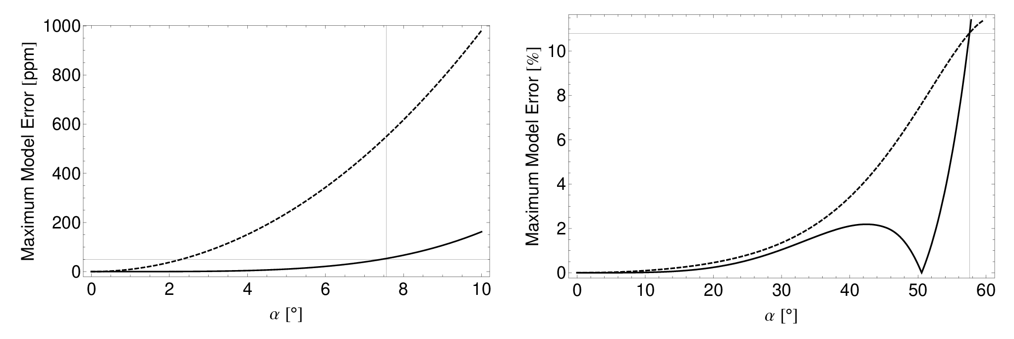
For simplicity, we assume the limb darkening of the spot and star are equivalent and set the spot-star contrast, , to be zero (a black spot). Numerically evaluating over the domain of interest reveals the error is maximised when . Therefore, we define .
The function grows with both and , tending to zero when they both equal zero, as expected. For a Sun-like star ( K, dex, [M/H] = 0), Claret (2011) estimate that the best fitting linear limb darkening coefficient in the Kepler bandpass is . One may now set to some desired tolerance level (e.g. the noise level of the data) and solve for i.e. the maximum spot size which leads to model errors below the tolerance level. We plot this function in Figure 3 (solid-line).
Since a star has a typical noise of ppm per long-cadence measurement (note that most Kepler targets are fainter than this), we estimate that the maximal error of our small-spot approximation is below that of a typical Kepler measurement error for starspots of angular radius . This corresponds to a spot coverage of %. Note that the modal spot coverage of stars in the Kepler sample is % (Basri et al., 2011). A 1.7% spot coverage roughly corresponds to on Figure 4 of Basri et al. (2011), which can be seen to encompass the majority of periodic variables. Given the conservative assumptions of using a relatively bright magnitude star (most Kepler targets are fainter), the fact that we assume only a single spot is responsible for the entire spot coverage (making the spot as large as possible) and the fact that the error derived is the maximal error rather than the typical error, we conclude that the large majority of spotted stars within the Kepler sample are appropriately modelled by the expressions in this work.
3.3 Model Error due to a Linear Limb Darkening Law Assumption
For larger spots, the modelling error becomes larger due to our small-spot assumption and thus an observer may opt to use the Dorren (1987) model instead. However, we point out that this model assumes a linear limb-darkening law which is somewhat unphysical in itself. The question therefore arises, at what point is the error in assuming a large spot with linear limb darkening better than assuming a small spot with non-linear limb darkening?
We have already calculated the error due to the small-spot assumption, assuming the star is perfectly described by a linear limb darkening law (). We may similarly define an error in assuming a linear limb darkening law when the star is really described by a non-linear law:
| (25) |
For a star with the same properties as used in the previous example ( K, dex, [M/H] = 0), Claret (2011) estimate that the best fitting non-linear limb darkening coefficients in the Kepler bandpass are . We also assume a black spot with the same limb darkening as the star, as was done for the previous example. Plotting the function for several realisations of as a function of , we find the maximal error occurs at . Thus we define .
In Figure 3, we plot this function along with as a function of for the Sun-like limb darkening coefficients computed by Claret (2000). The figure reveals that the error in assuming a small-spot is substantially smaller than the error in assuming a linear limb darkening law for , as one should expect. As an example, sunspots typically have angular sizes and for we find ppm whereas ppm i.e. our model is more than an order-of-magnitude more accurate. For spots of size we find ppm versus ppm.
We find that the significant error in assuming a linear limb darkening law does not become a better approximation than the small-spot model until , for Sun-like limb darkening. After this point, the error in our model rapidly tends to infinity and becomes untenable. The exact locations of the various turnovers and minima in Figure 3 depend upon the limb darkening parameters used. Also, the reliability of the function worsens for large since the “truth”, assumed to be itself starts to become erroneous at high .
Nevertheless, it is clear that our model is more accurate than the Dorren (1987) model for even a starspot equivalent to the largest spot ever detected (; Strassmeier 1999). Despite this, we would urge observers to use a numerical approach for such large spots since the model errors are significantly greatly than typical measurement errors. Spots of size should be well-described by the analytic model presented in this work.
4 An Example Application to Ceti
4.1 MOST observations of Ceti
Ceti is a relatively nearby G5 dwarf 9.1 pc from the Solar System. The star is notable for having a fairly rapid rotational period of 9 days and for being a bright Sun-like star at . MOST observations of Ceti in 2003 revealed the presence of two starspots with rotation periods of 8.9 d and 9.3 d (Rucinski et al., 2004). However, this single data set was insufficient to uniquely determine the latitudes of the spots and thus the differential rotation coefficient, could not be measured (the authors did not consider the -order coefficient ).
Subsequently, MOST observed Ceti two more times in 2004 and 2005 in order to gather enough data that a unique solution could be inferred. Indeed, this data, reported by Walker et al. (2007), was argued by the authors to be sufficient to locate a single minimum. The authors made use of the StarSpotz (Croll et al., 2006a) algorithm to regress the data, which in turn employs the Budding (1977) model for starspots (note that this is equivalent to the model of Dorren 1987). Starspotz locates the global minimum using parallel tempering and derives parameter posteriors using the Markov Chain Monte Carlo (MCMC) technique.
The photometry span three data sets, exhibit differential rotation and seven spots over three years (ranging from to ) and thus required considerable computational effort by Walker et al. (2007). For these reasons, the data make for an ideal test of not only our model here but for an alternative regressing technique.
4.2 Multimodal Nested Sampling with MultiNest
Nested sampling (Skilling, 2004) is a Monte Carlo method which puts the calculation of the Bayesian evidence in a central role, but also produces posterior inferences as a by-product. Nested sampling is generally considerably more efficient than MCMC methods for computing the Bayesian evidence of a model fit. For example, in cosmological applications, Mukherjee et al. (2006) showed that their implementation of the method requires a factor of fewer posterior evaluations than thermodynamic integration with MCMC. A full discussion of nested sampling is given in Skilling (2004) and Feroz et al. (2008) and for brevity we direct those interested to these works.
Multimodal nested sampling is an implementation of the technique to efficiently search parameter space under the assumption that one or more modes may exist in the data. Feroz et al. (2008); Feroz et al. (2009) describe multimodal nested sampling in detail, in particular in regard to their publicly available algorithm MultiNest. MultiNest is used by the “Hunt for Exomoons with Kepler” (HEK) project (Kipping et al., 2012) to compare the Bayesian evidence of a planet versus planet-with-moon regression. We will here demonstrate the use of MultiNest with our starspot model for the Ceti MOST photometry. Currently, MultiNest does not make use of the likelihood partial derivatives and so the partial derivatives were turned off in our implementation of macula. Since we only fit a single model through the data, there is no use of the Bayesian evidence here and thus we employ the constant efficiency mode of MultiNest at a target efficiency of 1% with 4000 live points.
4.3 Priors
In order to make a fair comparison to the Walker et al. (2007) result, we make the same assumptions as the original authors. Accordingly, we assume the same number of spots for each data set i.e. 2 spots for 2003, 3 spots for 2004 and 2 spots for 2005. The spots are assumed to be non-evolving over the course of each data set and have a lifetime which ensures they only exist within a single data set, as was assumed by Walker et al. (2007). We also assume for all and that the differential rotation profile is quadratic is nature (i.e. we fix ). Finally, limb darkening for the spot and the star are equivalent and follow a linear law governed by . Using these assumptions, we have the same number of free parameters (27) as was used by Walker et al. (2007).
The 27 parameters are 7 reference longitudes, , 7 reference latitudes, , 7 angular radii, , one equatorial rotation period, , one differential rotation coefficient, , one stellar inclination angle, and three instrumental offset terms, . Rather than label the offsets by , we use for each year. Since each year has unique starspots, we do use the spot labels but instead use &. These labels more clearly identify the spots associated with each year and follow the labelling notation of Walker et al. (2007). We adopt the uniform priors for all 27 parameters with the same range as that of Walker et al. (2007).
4.4 Results
The global maximum a-posteriori model fit is presented in Figures 4, 5 & 6 for the data sets in 2003, 2004 and 2005 respectively. Table 1 presents the posteriors of the best fitting mode and compares them side-by-side with the results reported by Walker et al. (2007).
| Parameter | Walker et al. (2007) | This Work |
|---|---|---|
| [∘] | - | |
| [days] | - | |
| - | ||
| - | ||
| - | ||
| - | ||
| [∘] | - | |
| [∘] | N/A | |
| [∘] | - | |
| [∘] | - | |
| [∘] | N/A | |
| [∘] | - | |
| [∘] | - | |
| [∘] | N/A | |
| [∘] | - | |
| [∘] | - | |
| [∘] | N/A | |
| [∘] | - | |
| [∘] | - | |
| [∘] | N/A | |
| [∘] | - | |
| [∘] | - | |
| [∘] | N/A | |
| [∘] | - | |
| [∘] | - | |
| [∘] | N/A | |
| [∘] | - |
As revealed in Table 1, the agreement between the derived system and spot parameters of Ceti is excellent with marginal differences between the estimates. The residuals of the fits in Figures 4, 5 & 6 closely match those of Walker et al. (2007). This therefore shows that macula coupled with MultiNest is capable of matching the results of StarSpotz.
Some remaining anomalies in the residuals are evident and one may be tempted to input more spots to fit these out. However, Walker et al. (2007) specifically caution against such a process arguing that the anomalies correlate to moon-light contamination and other instrumental effects.
Although it is not the focus of this work to explore the inter-parameter correlations and optimal fitting strategies, we here briefly comment on this issue. Our fits reveal the strongest correlations between values associated with the same data set i.e. the amplitudes of the signal components are correlated. We also find that the equatorial period, the stellar inclination and the individual latitudes exhibit mutual correlations, resulting from the uncertainty in the differential rotation determination.


5 Discussion
5.1 Performance
To test the speed of macula, we generated 1000 time stamps of a single synthetic input data set for a random choice of the star’s parameters. In all cases, full non-linear limb darkening is employed. We generate a single spot with random parameters and call macula 100,000 times to evaluate the typical execution time. Every call inputted random star and spot parameters in order to obtain a reliable average execution time. All simulations are run on a single-thread of a Intel Core i7 2.9 GHz processor with macula compiled in g95 using the optimisation flag -O3.
When macula is called, one may instruct the code whether to compute the partial derivatives. With derivatives turned off, macula requires 0.59 s per data point. Turning derivatives on yields 6.09 s per data point. Therefore, the act of turning on derivatives leads to a slowing down of the code by a factor of , for a single-spot model. Note that these times include the small overhead of generating random system parameters too.
Increasing the spot-number, we find that the no-derivatives call scales linearly with . However, the derivatives call exhibits super-linear, yet sub-quadratic, scaling of , or roughly . For this scaling, doubling the number of spots increases the CPU time by a factor of 3.34.
Due to its analytic nature, macula performs significantly faster than numerical codes made available in the literature. For example, Boisse et al. (2012) presented their numerical algorithm SOAP and report that generating 10,000 time stamps of a single synthetic starspot requires less than 40 s (but presumably close to this value). This indicates SOAP requires 4 ms per data point, compared to macula which requires 0.6 s per data point i.e. macula is around 6800 times faster than SOAP. There are several points which make a direct comparison somewhat unfair though. macula does not compute radial velocity variations, whereas SOAP does (although §5.3 shows how radial velocity variations are easily generated from the outputs of macula). Further, the authors used a slower 2.33 GHz Intel Core Duo processor for their benchmark tests. Nevertheless, it is clear that the difference in computation speeds is three orders-of-magnitude, making macula a powerful tool in inverse-problems.
5.2 Benefits
The analytic model for starspots presented here has several advantages which we list here:
-
An analytic algorithm for modelling photometric rotational modulation due to multiple circular, grey starspots, performing three orders-of-magnitude faster than comparable numerical codes.
-
Reproduces light curves with a maximum model error an order-of-magnitude less than that of the previous Budding (1977) and Dorren (1987) for a Sun-like non-linear limb darkened star observed in the Kepler bandpass, for spots of angular size .
-
Model accounts for spot contrast, non-linear limb darkening, differential rotation and starspot evolution.
-
Includes baseline normalisation parameters for data sets, as well as blended light dilution factors to aid in Kepler analysis.
-
Computes transit depth variations (TVs) due to unocculted spots.
-
Code is freely available as a Fortran routine, macula, located at www.cfa.harvard.edu/dkipping/macula.html.
5.3 Potential Applications
5.3.1 Rotational Modulation Measurements
We foresee several possible applications of macula. Firstly, measuring the rotational modulation of variable stars may be used to determine the rotation period, which may in turn constrain the ages of stars with gyrochronology (Barnes, 2009). Stars monitored with high signal-to-noise continuous photometry, such as that from Kepler, may also reveal differential rotation and the stellar inclination angle. An example of this type of regression is the analysis of Walker et al. (2007) for Ceti, where the inclination angle derived from rotational modulation alone and an analytic model for starspots yields a result fully consistent with the spectroscopic value. Note that we also reproduce this result using macula in this work. In addition, it may be possible to measure starspot evolution using the linear model employed by macula.
Rotational modulation analyses using macula are not limited to cool stars, which have been most commonly observed to exhibit such behaviour. There also exists evidence for spots on hot stars, such as the rapidly rotating B star HD 174648 (Degroote et al., 2011). Indeed, macula will also be applicable for bright spots on hot massive stars, such as those proposed by Cantiello & Braithwaite (2011) to explain observations of late O-type and early B-type stars made by CoRoT.
macula also produces predictions for the transit depth variations (TV) at any time stamp inputted. This may permit for the determination of rotational periods from TVs alone; highly useful for ground-based observations lacking the continuous photometry of space-based observatories. It may also be useful in testing whether observed TVs are consistent with starspots versus some other hypothesis e.g. planetary oblateness with precession (Carter & Winn, 2010).
5.3.2 Astrophysical Detrending
Due to the analytic nature of macula, the code is quick to execute and therefore many find uses in astrophysical detrending of photometry. For example, the PDC-MAP algorithm of Kepler is designed to remove instrumental trends but preserve the astrophysical signal, such as rotational modulation due to starspots. In performing a search for transits, or a detailed modelling of a known transit, detrending this rotational modulation is required. Whilst polynomial models or harmonic filtering may be used, an astrophysically-grounded model, such as macula, offers a viable alternative due to its fast execution time.
5.3.3 Radial Velocity Variations due to Starspots
We briefly remark that macula may be used to predict radial velocity variations due to starspots via the method described in Aigrain et al. (2012). Here, the authors propose that radial velocity variations can be reliably predicted from flux variations () alone. Specifically, the authors argue that the flux multiplied by its derivative in time reveals the radial velocity variations. macula returns both and for all input times (derivation provided in Appendix F).
5.3.4 Correcting Transmission Spectra
If a planet transits across a star, the atmosphere of the planet can reveal chromatic variations in the transit depth due to molecular absorption. In this way, transit measurements can reveal the “transmission spectrum” of an exoplanet. If the host star has unocculted starspots, one would expect to see chromatic variations in the depths purely from spots too, introducing a confounding signal. Further, transit depth measurements are often scattered both in wavelength and in time meaning that rotational modulation can also introduce spurious depth variations. Correcting for starspots is therefore a major challenge in studying the atmospheres of extrasolar planets. For example, Désert et al. (2009) found it necessary to use rotational modulation data of HD 189733 in order to correct Spitzer measurements of the planet’s transit depth.
macula offers a self-consistent way of modelling such corrections. Observations of rotational modulation may be used to directly infer TVs, provided the data are in the same bandpass as that used for the transit measurements. If the bandpasses differ (which is practically speaking likely), then one can estimate the depth variations by assuming a model for the spectral radiance of the starspots (e.g. blackbody). Nevertheless, we point out that obtaining several spectra within a few rotation periods of the intended transit measurement would be the most ideal way to correct for such activity, obviating the need for spectral radiance modelling.
5.3.5 Exomoon False-Positive Vetting
Whilst we leave the issue of modelling planet-spot crossings to future work, it is worth noting that such events may resemble exomoon mutual transits and are anticipated to be a source of false-positives in the “Hunt for Exomoon with Kepler” (HEK) project (Kipping et al., 2012). Even without detailed spot-crossing models, macula offers some simple tests to compare these two competing hypotheses. Firstly, the starspot coverage can be estimated from the out-of-transit variability, allowing one to gauge the feasibility of an observed anomaly being a spot-crossing event. Secondly, the derived rotation period from the rotational modulations can be used to check whether the light curve anomalies are consistent or inconsistent with such a period. Finally, Sanchis-Ojeda et al. (2012) (see Figure 1) have recently shown that the phase of a transit mid-time with respect to the rotational modulations () is related to the phase of a starspot with respect to the transit mid-time (). Any variations not matching this relationship would be difficult to explain as being due to a starspot.
Acknowledgments
We are grateful to Pieter Degroote for a very helpful review of our work. Special thanks to Bryce Croll & Gordon Walker for providing us with the MOST data of Ceti. Thanks to Jonathan Irwin, Roberto Sanchis-Ojeda amd Joel Hartman for very helpful conversations in preparing this work. DMK is funded by the NASA Carl Sagan Fellowships. This research made use of the Michael Dodds Computing Facility, courtesy of the HEK project.
References
- Aigrain et al. (2012) Aigrain, S., Pont, F. & Zucker, S. 2012, MNRAS, 419, 3147
- Basri et al. (2011) Basri, G. et al. 2011, AJ, 141, 20
- Barnes (2009) Barnes, S. 2009, IAU Symposium 258, 345
- Batalha et al. (2012) Batalha, N. M. et al. 2012, ApJS, submitted (astro-ph:1202.5852)
- Berdyugina (2005) Berdyugina S. V. 2005, LRSP, 2, 8
- Boisse et al. (2012) Boisse, I., Bonfils, X. & Santos, N. C. 2012, A&A, accepted (astro-ph:1206.5493)
- Budding (1977) Budding, E. 1977, Ap&SS, 48, 207
- Cantiello & Braithwaite (2011) Cantiello, M. & Braithwaite, J. 2011, A&A, 534, 140
- Carter et al. (2009) Carter, J. A., Winn, J. N., Gilliland, R. & Holman, M. J. 2009, ApJ, 696, 241
- Carter & Winn (2010) Carter, J. A. & Winn, J. N. 2010, ApJ, 716, 850
- Charbonneau et al. (2000) Charbonneau, D., Brown, T. M., Latham, D. W. & Mayor, M. 2000, ApJ, 529, 45
- Claret (2000) Claret, A. 2000, A&A, 363, 1081
- Claret (2011) Claret, A. & Bloemen, S. 2011, A&A, 529, 75
- Collier-Cameron et al. (1994) Collier-Cameron, A. & Unruh, Y. C. 1994, MNRAS, 269, 814
- Collier-Cameron et al. (1997) Collier-Cameron, A. 1997, MNRAS, 287, 556
- Croll et al. (2006a) Croll, B. et al. 2006a, in Bulletin of the American Astronomical Society, Vol. 38, Bulletin of the American Astronomical Society, 1217
- Croll et al. (2006b) Croll, B. et al. 2006b, ApJ, 648, 607
- Czela et al. (2009) Czesla, S., Huber, K. F., Wolter, U., Schroter, S. & Schmitt, J. H. M. M. 2009, A&A, 505, 1277
- Degroote et al. (2011) Degroote, P. et al. 2011, A&A, 536, 82
- Désert et al. (2009) Désert, J.-M., Sing, D., Vidal-Madjar, A., Hébrard, G., Ehrenreich, D., Lecavelier Des Etangs, A., Parmentier, V., Ferlet, R. & Henry, G. W. 2009, A&A, 526, 12
- Désert et al. (2011) Désert, J.-M. et al. 2011, ApJS, 197, 14
- Díaz-Cordovés & Giménez (1992) Díaz-Cordovés, J. & Giménez, A. 1992, A&A, 259, 227
- Dorren (1987) Dorren, J. D., 1987, ApJ, 320, 756
- Feroz et al. (2008) Feroz, F. & Hobson, M. P. 2008, MNRAS, 384, 449
- Feroz et al. (2009) Feroz, F., Hobson, M. P. & Bridges, M. 2009, MNRAS, 398, 1601
- Henry et al. (2000) Henry, G. W., Marcy, G. W., Butler, P. R. & Vogt, S. S. 2000, ApJ, 529, 41
- Hirano et al. (2012) Hirano, T., Sanchis-Ojeda, R., Takeda, Y., Narita, N., Winn, J. N., Taruya, A. & Suto, Y. 2012, ApJ, accepted (astro-ph:1205.3233)
- Kipping & Tinetti (2010) Kipping, D. M. & Tinetti, G. 2010, MNRAS, 407, 2589
- Kipping (2011) Kipping, D. M. 2011, MNRAS, 416, 689
- Kipping et al. (2012) Kipping, D. M., Bakos, G. Á., Buchhave, L., Nesvorný, D. & Schmitt, A. 2012, ApJ, 750, 115
- Kopal (1950) Kopal, Z. Harvard Coll. Obser. Circ., 454, 1
- Kron (1947) Kron, G, E. 1947, PASP, 59, 261
- Mandel & Agol (2002) Mandel, K. & Agol, E. 2002, ApJ, 580, 171
- Martínez et al. (1993) Martínez, P. V, Moreno, I. F & Vázquez, M. 1993, Astron. Astrophys, 274, 521
- McLaughlin (1924) McLaughlin, D. B. 1924, ApJ, 60, 22
- Mukherjee et al. (2006) Mukherjee P., Parkinson D. & Liddle A. R., 2006, ApJ, 638, L51
- Mullan (1974) Mullan, D. J. 1974, ApJ, 192, 149
- Nutzman et al. (2011) Nutzman, P. A., Fabrycky, D. C. & Fortney, J. J. 2011, ApJ, 740, 10
- Pál (2012) Pál, A. 2012, MNRAS, 420, 1630
- Petrovay & Van Driel-Gesztelyi (1997) Petrovay K. & Van Driel-Gesztelyi, L. 1997, Sol. Phys., 176, 249
- Rabus et al. (2009) Rabus, M. et al. 2009, A&A, 494, 391
- Rossiter (1924) Rossiter, R. A. 1924, ApJ, 60, 15
- Rucinski et al. (2004) Rucinski, S. M. et al. 2004, PASP, 116, 1093
- Rüdiger & Kitchatinov (2000) Rüdiger, G. & Kitchatinov, L. L., 2000, Astronomische Nachrichten, 321, 75
- Russell (1912) Russell, H. N. 1912, ApJ, 36, 54
- Sanchis-Ojeda et al. (2011) Sanchis-Ojeda, R., Winn, J. N., Holman, M. J., Carter, J. A., Osip, D. J. & Fuentes, C. I. 2011, ApJ, 733, 127
- Sanchis-Ojeda et al. (2012) Sanchis-Ojeda, R. et al. 2012, Nature, 487, 449
- Skilling (2004) Skilling, J. 2004, in Fischer R., Preuss R., Toussaint U. V., eds, American Institute of Physics Conference Series Nested Sampling. pp 395–405
- Sing et al. (2009) Sing, D. K., Désert, J.-M., Lecavelier Des Etangs, A., Ballester, G. E., Vidal-Madjar, A., Parmentier, V., Hebrard, G. & Henry, G. W. 2009, A&A, 505, 891
- Slawson et al. (2011) Slawson, R. W. et al. 2011, ApJ, 142, 160
- Skumanich (1972) Skumanich, A. 1972, ApJ, 171, 565
- Stix (2002) Stix, M. 2002, Astronomische Nachrichten, 323, 178
- Strassmeier (1999) Strassmeier, K. G. 1999, A&A, 347, 225
- Tuominen et al. (2002) Tuominen, I., Berdyugina, S. V. & Korpi, M. J. 2002, AN, 323, 367
- Walker et al. (2007) Walker, G. A. H. et al. 2007, ApJ, 659, 1611
- van Leeuwen et al. (1997) van Leeuwen, F., Evans, D. W., Grenon, M., Grossmann, V., Mignard, F. & Perryman, M. A. C. 1997, A&A, 323, 61
- Vogt (1975) Vogt, S. S. 1975, ApJ, 199, 418
- Vogt & Penrod (1983) Vogt, S. S. & Penrod, G. D. 1983, PASP, 95, 565
Appendix A Geometry of the Spot
A.1 Position of the Spot
The basic unit of our model is a circle, which represents a starspot, on the canvas of a star’s surface. We begin by considering a single starspot and show later how the result is generalised to multiple spots. We will assume that the star is perfectly spherical in what follows. The geometry of the spot is characterised by a position and a size. The position, which we define as the position of the starspot’s centre relative to the centre of the star, must be a two-dimensional vector given that a surface has a two-dimensional topology. An appropriate positional vector would be longitude () and latitude (). We define these terms to exist in the range and .
We initially consider the centre of the spot to be located in a Cartesian frame at a location given by the unit vector (where we adopt units of the stellar radius). In all frames of reference, we consider the observer to be located along the -axis at .
The centre of the spot can be described at any longitude and/or latitude by multiplying the unit vector by two rotation matrices, accounting for longitude and latitude. At this stage, we denote the longitude and latitude using the notation and respectively, which we dub “apparent longitude” and “apparent latitude”. This is done in order to reserve the symbols and (the true longitude and latitude) for later when we will account for stellar inclination as well. The rotation matrices for apparent longitude and latitude are defined by the notation then , respectively.
Consider that the action of these two rotation matrices leads to a position for the centre of the spot defined by the vector . Due to the non-commutative nature of linear algebra, the order in which one chooses to perform these rotations will affect the results. Here we follow historical precedent and define:
| (26) | ||||
| (27) |
where we have
| (28) |
| (29) |
One may combine the two matrices into a general transformation matrix, , given by
| (30) |
We use this matrix to determine
| (31) |
A.2 Size of the Spot
We wish to define the radius of the spot in terms of a solid angle swept out from the centre of the star. Let us define this solid angle to be given by . A spot of solid angle radius radians would reach from pole-to-pole and thus we define . Later when we account for limb darkening effects (§C.2), we show that it is necessary to assume and this should be interpreted as the hard-limit of our model, macula.
For a starspot with a position vector described by , it is trivial to show that the apparent radius of the spot would be . In this frame, the spot appears as a perfect circle on the - plane.
A.3 Rim of the Spot
We define the rim of the spot to be those points which lie along the two-dimensional projected perimeter of the starspot, when viewed along a vector normal to the stellar surface and passing through centre of the starspot (i.e. when ). After applying the rotation matrices to account a starspot’s apparent longitude and/or latitude, the position vectors describing the loci of points along the rim are transformed too.
Let us define the position vector of the loci of points along the rim, when viewed in the frame such that , by the vector . After accounting for the spot’s apparent longitude and latitude, we use the vector .
For , the loci of points may be described using parametric equations, taking advantage of the fact the projection of the spot is a perfect circle (as described in the previous subsection).
| (32) |
where traces the loci of all points along the starspot rim. We may now apply the rotation matrix to find the parametric expressions describing the rim for any apparent longitude or latitude, thereby accounting for the fore-shortening effect.
| (33) |
which may be shown to yield
| (34) | ||||
| (35) | ||||
| (36) |
A.4 Bulge of the Spot
Consider again the frame in which one views the spot down the vector normal to the stellar surface and passing through the spot’s centre. In the model described in this work, the spot lives in three-dimensions in a Cartesian framework. Notably, the spot exhibits a bulge due to the curvature of the stellar surface. From the perspective of the star’s centre, the loci of the points on this bulge can be described by two angles; a radial angle, , and an azimuthal angle, . We may define these loci by again starting from the frame in which , and applying rotation matrices appropriately. In this simple frame, we define the position vector for the loci of the points existing on the bulge as
| (37) |
where we have
| (38) |
| (39) |
Here the radial angle, , is bound to be i.e. it cannot subtend an angle greater than the solid angle radius of the spot. The azimuthal angle has the freedom to be . We use these matrices to determine:
| (40) |
Note the dash, which (as before) is used to denote that this is derived in the frame not accounting for a spot’s apparent longitude and/or latitude. As was done earlier, we may now apply the longitude-latitude rotation matrix, , to account for any orientation desired:
| (41) |
which gives
| (42) | ||||
| (43) | ||||
| (44) |
A.5 A Useful Simplification
Due to the circular symmetry of the problem, it is actually degenerate to use two angles to describe the position of the spot. All that matters is how close to the spot is to the limb, regardless as to the combination of longitude and latitude responsible. For this reason, we may define any combination of these terms using a single “auxiliary angle” we dub (in-keeping with the notation of Dorren 1987).
The angle of interest is the angle subtended between the vector (pointing towards the observer) and the vector describing the position of the spot’s centre relative to the centre of the star . Let us define this as the auxiliary angle . can be found by using the dot-product rule of these two relevant vectors:
| (45) |
Since is a unit-vector in the -direction, then this dot-product simply extracts the -component of . Therefore we have:
| (46) |
which may be evaluated here to be
| (47) |
may also be thought of as being like a net longitude shift at zero latitude i.e. and .
Due to the mirror symmetry of the problem, we only need consider to derive all possible scenarios. The vectors of interest now become, without any loss of generality,
| (48) |
| (49) |
| (50) |
Appendix B Four Cases
B.1 Overview
B.1.1 Case I
In order to compute the flux from a starspot, we need to compute the projected area in the - plane. It can be easily seen that four distinct cases exist for the geometry of the rim and bulge. The most obvious case is the dominant source of flux variations since the spot is nearly face-on. For between 0 and some angle close to the limb of the star, the loci of points on the bulge lie fully inside the rim of the starspot, as seen in the projected - plane. This case is trivial to model and the rim expressions may be used alone to compute the area of the starspot. Case I is valid for where we are yet to define but it can be understood to be angle close to the limb of the star.
B.1.2 Case II
Case II occurs as approaches from . It is defined as when the loci of points on the bulge are no longer contained within the projected rim of the starspot. Since the bulge has a -component, as we rotate round in longitude, this -component will be transferred into an ever-increasing -component. Eventually, this -component exceeds the rim’s maximal -value at which point “the bulge pokes out of the rim”. Case II is valid for .
B.1.3 Case III
Case III occurs as increases beyond i.e. the centre of the spot is behind the star. However, a portion of the starspot is still in view and causes a flux decrement. It can be easily understood that once exceeds then the spot has fully disappeared behind the back of the star. Thus, case III is valid for .
B.1.4 Case IV
Case IV is simply the case of the spot fully behind the star and thus there is no contribution to the model flux. This is valid for (recalling that is defined only within the range due to the mirror symmetry of the problem).
B.2 Case II
B.2.1 Optimal Bulge Curve
We here devote a section to case II alone, due to the non-trivial nature of solving for its parametric equations. We first start by defining the “optimal bulge curve”. For any co-ordinate of a point lying within the bulge, the optimal bulge curve is the corresponding co-ordinate which maximises . It is the curve which seems to extend furthest to the limb of the star, as seen in the transformed frame. Since all loci on the 2D surface of the bulge are defined by two parametric terms ( and ), it should be clear that the parametric equation of the optimal bulge curve will require only one term; either or , but not both. We arbitrarily choose here to define our optimal bulge curve purely in terms of .
The optimal bulge curve also exhibits the greatest separation from , relative to all other loci on the bulge. Thus we expect that is maximised and so:
| (51) |
Solving the above for yields two solutions, only one of which is the maximum:
| (52) |
where we only consider the range and here (the latter due to the case II conditions and the former due to symmetry about the -axis). This yields the following parametric expression in the - plane:
| (53) | ||||
| (54) |
Evaluating the equation for at reveals . Thus, when the optimal bulge curve intersects the -axis, although we note that at this point the corresponding point may be exceed and thus may not truly exist on the bulge. However, it reveals that increases as increases form 0 to .
B.2.2 Intersection of Optimal Bulge Curve and the Rim
For case II, where , there exists a certain point where the optimal bulge curve intersects the starspot rim. We denote this location as . The location corresponds to a unique parametric location along the rim, . Similarly, there exists a unique parametric location along the optimal bulge curve, .
Let us deal with first. Since the optimal bulge curve extends outside the rim, this location can be shown to occur when the rim’s - distance from the origin is maximised i.e. when is maximised. We therefore must solve the following expression for :
| (55) |
which may be shown to yield:
| (56) |
The intersection point along the optimal bulge curve can be found by minimising the distance on the - plane between the optimal bulge curve and the rim. Therefore, we must solve the following expression for :
| (57) |
which yields the following solution:
| (58) |
Feeding this back into the expressions for the optimal bulge curve, we locate the Cartesian co-ordinates of the intersection point:
| (59) | ||||
| (60) |
where it is again understood this is for the range only.
B.2.3 The Critical Angle,
As discussed earlier, for and increases up to a maximum at . Similarly, by definition the parametric expression for is maximised for . Case II is only valid for a bulge which pokes out of the rim and its boundary will occur for . Solving for , we find:
| (61) |
This therefore proves an intuitive point. The optimal bulge pokes out of the rim when the rim hits the edge of the star. At this instant, the starspot rim makes contact with the projected rim of the star and the optimal bulge is just a single point at . As becomes larger, the starspot rim gradually disappears behind the back of the star and the optimal bulge curve spreads out along the projected rim of the star.
B.2.4 Projected Area of the Starspot: I. The Rim
The projected area of the starspot, for case II, can be thought of as the sum of the projected area bound by the rim and that of the bulge poking out, with the transition occurring at the intersection points derived. The rim therefore bounds an area between . We consider here the area above the -axis only, which can later be simply doubled due to symmetry about the -axis.
We start by re-writing the expression for to make the subject:
| (62) |
We may now replace the in to obtain :
| (63) |
The area bounded by the rim is therefore given by:
| (64) | ||||
| (65) |
B.2.5 Projected Area of the Starspot: II. The Bulge
We now need to repeat this process for the optimal bulge curve. One may re-write the expression for making the subject:
| (66) |
Feeding this into the expression for in order to obtain we obtain the simple solution:
| (67) |
Once again, this result proves the same inuitive result we saw earlier. Specifically, the optimal bulge curve lies along the projected rim of the star itself. The bounded area is given by:
| (68) | ||||
| (69) |
B.2.6 Projected Area of the Starspot: Total
Combining these two results together, we obtain the area of a circular starspot under case II conditions:
| (70) | ||||
| (71) |
B.3 Case III
B.3.1 Edge Bulge Curve
For case III, we have . Here, the centre of the spot is out-of-view, hidden behind the star. Despite this, a portion of the spot’s surface remains at and thus is still visible. For case II, we defined an optimal bulge curve which tracked the curve of interest. Similarly, here we define the “edge bulge curve” to the perimeter of the bulge still in view when case III conditions remain in effect.
The edge bulge curve is much easier to define that the optimal bulge curve. For the range , it is simply given by maximizing . Since is bound to be , then . Thus, the parametric equations describing the edge bulge curve are:
| (72) | ||||
| (73) | ||||
| (74) |
B.3.2 Boundary of the Edge Bulge Curve
The edge bulge curve intersects the stellar rim when the quadrature sum of the and components equals unity. Therefore, we may find the value of this location, which we dub , by solving the following expression for :
| (75) |
which yields:
| (76) |
Plugging the above into our expressions for yields :
| (77) | ||||
| (78) | ||||
| (79) |
The right-most -point occurs when we cross the -axis i.e. when . It is trivial to show this occurs for and correspondingly .
B.3.3 Area Bounded by the Edge Bulge Curve
Taking the expression for , we may re-write this to make the subject via:
| (80) |
We may feed this into to obtain :
| (81) |
Due to the concave nature of the edge bulge curve, the area of the loci of points on the bulge only is defined by:
| (82) |
Finally, one may express this purely as a function of and :
| (83) |
B.4 Cases I & IV
B.4.1 Case I
For completion, we here briefly derive the expressions for cases I and IV. Case I has the spot fully in view at some angle where . The relevant parametric equations are the rim expressions derived earlier. The area may be found to be:
| (84) |
B.4.2 Case IV
Case IV is for and corresponds to the spot fully out-of-view behind the star. The case trivially has an area:
| (85) |
Appendix C Modelling the Light Curve
C.1 For a Uniform Brightness Star
C.1.1 Generalising to a Single Domain Function
It can be easily shown that these expressions produce the same light curve profile predicting by Dorren (1987) in the absence of limb darkening and a black spot.
The expressions for and possess some similarities in form and are of course continuous at the point . This led us to investigate if the two equations are equivalent to some simplified form. We found the following expression describes both and :
| (86) |
where
| (87) |
Encouraged by this, we tried plotting the function in the range . However, becomes complex in this range. We therefore only considered the real part. It is easy to see by example that the real part of perfectly maps the function.
A final success of comes from considering the case IV range i.e. . Here the real part of goes to zero but the imaginary component gradually increases. Thus, by plotting the real part of only, we can reproduce all four cases with a single function across the full domain of . Thus, we have:
| (88) |
The advantage of using this single-domain function is that we can define an analytic Jacobian and Hessian matrices, which are useful in expediting regression of photometric data. macula will provide the Jacobian, but not the Hessian to save computation time (although it may be extended to perform this function too due its analytic form).
C.1.2 Model Flux
For a single-rotating spot on a uniform brightness star, the flux from a star () can be computed using:
| (89) |
where denotes flux-per-unit-area and is the area of the spot. Photometric observations are usually normalised to some arbitrary value. A suitable choice here is the flux from the star in the absence of a starspot i.e. .
| (90) |
where and is the flux-contrast of the spot relative to the star. It may also be thought of as a proxy for the temperature of the spot. For non-overlapping starspots labelled , this can be extended to:
| (91) |
which yields
| (92) |
C.2 For a Limb Darkened Star
C.2.1 The Mandel-Agol Cases
In this work, we will assume that the size of the spot is small relative to the size of the star. This approximation allows us to easily write down analytic functions for the light curve and follows on from the work of Mandel & Agol (2002) and Kipping (2011). Specifically, we will use the small-planet approximation from Mandel & Agol (2002) and utilise 4-coefficient non-linear limb darkening. The flux from a star in the absence of starspots is therefore modelled via Equation 10 provided earlier:
| (93) |
where are the limb darkening coefficients, , is the normalised radial coordinate on the disk of the star and is the specific intensity as a function of , with .
Limb darkening is present over the entire viewable surface of the star, including those portions which are covered in starspots. However, due to the different temperature and opacity of this surface, the limb darkening coefficients cannot be assumed to be necessarily the same as that for the rest of the stellar surface. We therefore consider the specific intensity of the spot covered surface to be described by limb darkening coefficients , , and :
| (94) |
Note how we assume is not a function of position on the star’s surface or equivalently the spot’s radial angle, . In other words each spot has a uniform temperature, although the temperature may vary between spots. Also, §2.4 describes how umbra/penumbra may be generated using our model allowing for a more complex profile.
For a single rotating spot, we will denote the model flux as being composed by the following components:
| (95) |
The obscured and total flux components are computed as one would do so for a transiting planet model. In this scenario, there are four principal cases, as shown in Table 2. The table requires we define an angle at which point the spot no longer covers the centre of the star (M3-M9 boundary). When does this occur?
In order to simplify the problem, let us assume it is not possible for a spot to both cover the stellar centre and to exceed the angle . This is equivalent to assuming . For the loci of points along the rim of the starspot, the locus which is closest to the sky-projected stellar centre has a position . Therefore, when , the spot no longer covers the stellar centre. The spot therefore no longer covers the stellar centre once and this is the critical angle of interest required for deriving our limb darkening model.
| Case | Analogous Condition for a Planet | Condition for a Spot | Range |
|---|---|---|---|
| M1 | Case IV | ||
| M2 | Cases II & III | ||
| M3 | Case I | ||
| M9 | Case I |
C.2.2 Case M3
For case M3, it may be shown (see Kipping 2011) that:
| (96) |
For the spot, we must compute the flux obscured by its presence. This can be done by exploiting of the circular symmetry of the limb darkening effect and integrating the flux over an annulus defined to have an inner radius equal to the left-most point of the spot and outer radius equal to the right-most point of the spot.
| (97) |
Note that the solution above has a significantly more compact form that than acquired for an exomoon in Kipping (2011). We may correct for the fact this is the flux over the entire annulus by applying:
| (98) |
where and have been previously defined.
Finally, we need to compute , the flux from the spot itself. As will be the situation for all cases, the derivation for is precisely the same as that as was done for except that and we multiply the expression by to account for the temperature difference:
| (99) |
where the label emphasises that it is valid for all cases.
C.2.3 Case M9
M9 considers the case when the spot overlaps with the centre of the stellar disc. Here, we must adjust the integration limits of the annulus flux since :
| (100) |
Correcting for the expanded annulus area, we find:
| (101) |
C.2.4 Case M2
M2 considers the case when the spot now hits the stellar limb. Again, we must adjust the integration limits of the annulus flux since :
| (102) |
Correcting for the expanded annulus area, we find:
| (103) |
C.2.5 Case M1
The final case, and the simplest, is when the spot is out-of-view, analogous to the out-of-transit planet. Here, we have:
| (104) |
C.2.6 Final Expressions
For a single rotating starspot, satisfying the assumptions made in this work, we find that the flux from a star with a starspot may be written as:
| (105) |
where
| (106) |
and
| (107) |
In the above form, the expressions span two/three domains. A single-domain function can be expressed using Heaviside Theta functions, :
| (108) |
Or more generally:
| (109) |
where and .
Equation 105 may be shown to return Equation 90 if one sets , as expected. For Equation 90, we showed how it was trivial to generalise the expression to spots, provided one assumes the spots do not overlap. The same extension may be used here to yield:
| (110) |
where the expressions for are trivially generalized to by amending and . Note that in the above expression we have added a Kronecker Delta function. This is because for , the fraction containing the terms goes to i.e. undefined. Adding the Kronecker delta instead causes this to be equal to in this special circumstance and thus adds numerical stability to the function.
C.3 Expressing with Physical Parameters
C.3.1 Accounting for the Star’s Geometry
So far, we have derived an expression for the flux from a limb-darkened star covered in multiple spots of sizes and instantaneous positions , as given in Equation 110. It was shown earlier how could be related to a specific choice of apparent longitude, , and apparent latitude, , via Equation 46:
As stressed throughout, and are the apparent longitude and latitude of a starspot. The vector describing the Cartesian coordinates of the spot’s centre is and so far we have only defined this as a function of and i.e. we know . However, here we show how the vector can also be expressed as a function of the true longitude and latitude (i.e. accounting for the star’s geometry), . This is crucial since the flux from the star is described by the parameters and only and ultimately one wishes to describe the flux as a function of the physical parameters and not auxiliary angles.
Consider a frame in which the geometry of the star is such that the rotation axis has a normal vector given by i.e. along the -axis. In this frame, the apparent longitude and latitude are in fact equal to the true longitude and latitude, by virtue of definition. In this frame, which does not account for stellar geometry, we describe the position vector of the spot’s centre with vector . Due to the argument made above, we have:
| (111) |
or explicitly
| (112) |
In order to calculate , we must transform the frame to account for the geometry of the star. In other words we seek to transform .
Euler’s rotation theorem states that any large series of three-dimensional rotations can be written as a series of just three rotations only. Two conventions exist for how these three “Euler rotations” may be performed. The first is known as “proper Euler angles’. According to the intrinsic/extrinsic rotation equivalences, proper Euler angles are equivalent to three combined rotations repeating exactly one axis e.g. --. The second convention is called the “Tait-Bryan angles” (also known as the “Cardan angles”) and these are equivalent to three composed rotations in different axes e.g. --.
We abstain from choosing a convention for the moment and proceed to consider a sequential choice of rotations which minimises the degeneracy between the various angles. We note that by choosing the first axis to be , we can eliminate a redundant angle since we defined an initial configuration with the stellar rotation axis aligned to the -axis (i.e. an initial rotation is equivalent to intrinsic stellar rotation). For the sake of completeness, we refer to this first rotation as a clockwise rotation about the -axis by an angle .
For the next rotation, it is desirable to include stellar inclination at this point. A clockwise rotation about by an angle would correspond to the traditional definition of the stellar inclination angle. We have now selected the first two rotations, leaving just to the third. If we follow the proper Euler angles, we will be forced to us a rotation. In contrast, the Tait-Bryan convention would require a rotation. Since the observer is located down the -axis, a rotation about this axis cannot change the observed disk-integrated flux. Thus, a rotation about this axis would be redundant. For this reason, we use the Tait-Bryan convention and define our Euler rotation scheme as -- leading to two redundant angles and only one angle of physical interest, (for completeness we dub the rotation angle as ). We therefore define the position of the starspot centre, after applying the Tait-Bryan rotations, as:
| (113) |
where the first rotation is a clockwise rotation about the -axis by an angle :
| (114) |
The second rotation is a clockwise rotation about the axis by an angle .
| (115) |
Finally, the third Euler rotation is about the -axis in a clockwise sense by an angle .
| (116) |
Recall from Equation 46 that the -component of directly yields , via
| (117) |
Applying all three rotations and extracting the -component allows us to write as a function of the true longitude and latitude:
| (118) |
As discussed earlier, and manifestly evident from the above expression, the angle is fully degenerate with and thus may be neglected, giving us:
| (119) |
It may be easily seen that this is precisely the same expression as Equation 8 of Dorren (1987).
C.3.2 Accounting for the Star’s Rotation
Stellar rotation causes the a spot’s instantaneous longitude to vary as a function of time. We denote the rotation rate by , where is the rotational period of the star. Although it may be possible to envisage spots which migrate in latitude as well as longitude, we here only consider the simple case of and . We may then decsribe the spot’s instantaneous longitude and latitude as a function of time using:
| (120) | ||||
| (121) |
C.4 Differential Rotation
In general, unique terms are included to allow for differential rotation. However, differential rotation is well-described by the following function:
| (122) |
The is usually only used for Solar rotation analysis, but we include it here for cases where a user requires a more soPhisticated differential rotation profile.
C.5 Starspot Evolution
C.5.1 A Linear Model
There is some debate in the literature regarding how to model the evolution of a single starspot. Rüdiger & Kitchatinov (2000) show that the theoretical decay rate from 2-D modelling of a sunspot is close to linear for the spot area (i.e. a square-root rate for ). Similarly, Stix (2002) argue that if the decay of an isolated sunspot is set by the amount of the azimuthal electric current within the spot, a linear decay in area would result. However, Petrovay & Van Driel-Gesztelyi (1997) use a statistical analysis of sunspot data to show that an “idealised” sunspot exhibits parabolic area decay. Additionally, observations of Martínez et al. (1993) find both linear and parabolic decays.
With our model, the user is free to use any description they desire, but the code provided considers a simple linear growth/decay in model and the partial derivatives computed are only valid for said model.
A linear model has the advantage of being intuitively simple to handle, making the selection of appropriate boundary conditions and starting points easier for regression problems. It is also very quick to computationally evaluate and encapsulates the key physics involved. Our linear model produces a linear growth, flat-top and then linear-decay i.e. a trapezoidal profile for the spot’s evolution. The profile is allowed to asymmetric to reproduce realistic evolution.
We model starspot growth/decay via the parameter only i.e. we consider the flux contrast to be constant. The linear-model has the simple form:
| (123) |
and using
| (124) | ||||
| (125) | ||||
| (126) | ||||
| (127) |
where is the Heaviside step function, is the maximum spot-size, is the full-width-full-maximum “lifetime” of the spot and & are the ingress & egress durations of the spot profile.
C.6 Normalisation and Blended Light
As discussed earlier, we choose to normalise the flux of spotted star by the flux which the same star would cause if no spots were present i.e.
| (128) |
At the time of writing, the most precise and sizable source of photometric time series for main sequence stars comes from Kepler Mission. With this in mind, we choose to include a blending factor at this stage to account for overlapping PSFs, background flux or flux from an associated member in the system. This is a fairly common occurrence for Kepler data and many other photometric surveys due to the crowded fields observed. Let us consider then that the total flux observed is changed via . Our normalisation factor must now also be modified if we require that for an unspotted star. An appropriate choice is to use :
| (129) |
Using is cumbersome and a more common approach is to define a blending factor, relative to the target’s flux. Kipping & Tinetti (2010) advocate using which we follow here. This yields:
| (130) | ||||
| (131) |
C.7 Allowing for Multiple Time Series
In many practical cases, we must fit multiple epochs of data which have different systematics. The most common systematic to be treated is a baseline parameter, . A common application of this process is using a unique normalisation factor for each Kepler quarter since spacecraft rolls affect the total flux within a defined aperture. For data sets (e.g. quarters of data from Kepler), each set requires a unique parameter. Using a box-car function (), which is a composite of two Heaviside Theta functions, one can reproduce the desired behaviour:
| (132) | ||||
| (133) |
where it is understood that . Note that we have also assumed that each data set has a unique blending factor. For Kepler data, it is typical for each quarter to have a unique factor from spacecraft motion altering the PSF overlaps.
Consider we have two data sets separated by rotation periods where . Further assume that the time span of data sets 1 and 2 are shorter than the spot lifetime of all spots i.e. for all and . In this case, may one wish to treat the spots in data set 1 as independent of data set 2. This can be implemented by making use of the starspot evolution equations. Specifically, one wishes to impose box-car spots (unchanging during each data set) with cut-offs in-between the two data sets. So the starspot of the data set will have take the form and and .
Appendix D Partial Derivatives
D.1 Motivation
One of the major benefits of writing our expression as a single-domain function is that one can consider writing down a set of a single-domain partial derivatives. Partial derivatives are highly useful in optimisation problems where frequently the Jacobian matrix is computed to expedite a regression problem.
D.2 Partial Derivatives of the Likelihood Function
The commonly used Gaussian noise likelihood has the form:
| (134) |
Taking the partial derivative of the log likelihood with respect to parameter yields:
| (135) |
where . Also note that in the above, and what follows throughout, that any partial derivatives taken with respect to implicitly means that all other parameters are held constant except . In other words, for a set of parameters where , we use the notation that the partial derivative of some quantity follows
| (136) |
The outstanding problem is to derive , which we deal with in the next subsection. We point out that any reasonable likelihood function, even if non-Gaussian, will still require . For this reason, in the provided code macula, we do not provide the partial derivatives of a Gaussian likelihood function directly but instead provide the partial derivatives of the model flux instead, . In this way, the results from macula are more general and hopefully of greater use to typical observers.
D.3 Partial Derivatives of the Model Flux
Recall our final expression for the model flux, evaluated for the data point:
| (137) |
which may be written as
| (138) |
So one may easily see that
| (139) |
The function now requires partial derivatives. We adopt the assumption that is not a function of any of the parameters. This is perfectly reasonable as the function is only a function of and , which the user would define rather than fit for. Using this assumption, for all . Using the replacement (purely to save space) that and , one may now show:
| (140) |
The above expression shows that the partial derivatives of the model flux can be expressed as a function of four other partial derivatives (which in turn may be broken down into other partial derivatives).
and in particular are functionally dependent upon many parameters but and do not. Rather, they represent a fitted parameter and have no other dependencies. We therefore have:
| (141) |
and
| (142) |
With these expressions the only remaining partial derivatives to find are those of and . In fact, since is defined as simply a special case version of then we only require solving the partial derivatives of or equivalently .
D.4 Partial Derivatives of the Flux w.r.t. Limb Darkening
The function is fully expressed as:
For an unspotted star, for all & and so one may write:
| (143) | ||||
| (144) | ||||
| (145) | ||||
| (146) |
This allows us to write that
| (147) |
It is easy to show that
| (148) |
D.5 Partial Derivatives of
The outstanding problem is now to find the partial derivatives of with respect to . is defined as:
We therefore proceed to derive the full four-coefficient partial derivatives, which we start by re-writing:
| (149) | ||||
| (150) |
For the complex function , the only derivatives of interest are with respect to and since is functionally dependent on these terms alone. It may easily shown and numerically verified that:
| (151) | ||||
| (152) |
Since all other partial derivatives of can be expressed using the chain rule as a combination of the above two forms, then partial derivatives of can be derived for all using this simple trick. This allows us to write:
| (153) |
With the above, one can see the outstanding problem is to find partial derivatives of & with respect to .
D.6 Partial Derivatives of
is a function of and only. Whilst these two terms will be functions of other parameters themselves, they offer the obvious starting point for a derivation of ’s partial derivatives. The partial derivatives with respect to and are easily shown to be given by:
| (154) | ||||
| (155) |
where we use
| (156) |
One may now employ the chain rule to write:
| (157) |
where we temporarily re-include the implicit notation to make the expression less ambiguous. Partial derivatives of & with respect to will be provided later.
D.7 Partial Derivatives of
is fully expressed as:
| (158) | ||||
| (159) |
We first turn our attention to taking the partial derivatives of with respect to . We note that that:
| (160) | ||||
| (161) |
which via the chain rule imply:
| (162) |
With this simplification, we find:
| (163) |
The partial derivatives of are given by:
| (164) | ||||
| (165) |
and of
| (166) | ||||
| (167) |
In practice, the functions always yield zero unless . Since they are a function of a continuous variable, namely time, the probability that the time will precisely yield a non-zero function is infinitesimal. For this purpose, they are simply ignored in the macula code. The latter relations lead to a simplification of the chain rule expansion of the partial derivatives with respect to :
| (168) | ||||
| (169) |
Finally, the partial derivatives of are:
| (170) |
Since the partial derivatives of have been dealt with above, this leaves us to comment on the partial derivatives of , and . These represent fitted parameters (or perhaps fixed) and thus one may trivially evaluate their derivatives to be
| (171) |
| (172) |
| (173) |
D.8 Partial Derivatives of
The only partial derivatives now missing are those of and with respect to the fitted parameters, . is defined as:
Accounting for differential rotation, the longitude evolution is described by:
| (174) |
Now the partial derivatives yield:
| (175) | ||||
| (176) | ||||
| (177) | ||||
| (178) | ||||
| (179) | ||||
| (180) |
Aside from the above, the remainder of the partial derivatives satisfy:
| (181) |
D.9 Partial Derivatives of
The starspot evolves via Equation 5. The partial derivatives are found to be:
| (182) | ||||
| (183) | ||||
| (184) | ||||
| (185) | ||||
| (186) |
Aside from the above, the remainder of the partial derivatives satisfy:
| (188) |
Finally, it is necessary to define a reference longitude, . A convenient choice is to define it as the longitude at the instant , which is the default assumption of macula.
Appendix E Manipulating Partial Derivatives
E.1 Alternative Limb Darkening Laws
In this model, we have adopted the four-coefficient limb darkening proposed by Claret (2000). Several, but by no means all, alternative limb darkening laws can be adopted by re-parametrising the four-coefficient model presented in this work. In this subsection, we discuss four examples: i) the quadratic law (Kopal, 1950) ii) the linear law (Russell, 1912) iii) the three-coefficient law (Sing et al., 2009) iv) the square-root law (Díaz-Cordovés & Giménez, 1992). In each case, we show how one may use the results from macula to obtain the partial derivatives for regression purposes. In what follows, we assume that the spot and the star have distinct limb darkening coefficients.
E.1.1 Quadratic Law
The quadratic law, first proposed by Kopal (1950), is perhaps the most commonly adopted model in the exoplanet literature. Recall from Equation 10 that the four-coefficient limb darkening law is described by
In contrast, the quadratic law is described by
| (189) |
By comparing the coefficients relative the four-coefficient model, one may show that the quadratic law may be reproduced by setting:
| (190) |
The quadratic model is popular in the exoplanet community when one wishes to fit for the limb darkening parameters. The reason for this is two-fold. Firstly, photometric data are rarely precise enough to regress a unique solution for all four coefficients of the non-linear limb darkening law and so using the quadratic model reduces the number of free parameters by two yet preserves curvature in the intensity profile of the star. Secondly, the two quadratic coefficients, and , have well-described priors by imposing that the intensity profile is monotonic and everywhere positive. Carter et al. (2009) show that these conditions impose
| (191) |
Kipping et al. (2012) point out that a sensible upper-bound on may be imposed from inspection of typical coefficient tables presented in works such as Claret (2000). A typical choice is for Sun-like stars. With this upper-bound one may re-define and regress the parameters subject to the uniform priors:
| (192) |
The four-coefficient model can be set to these parameters using:
| (193) |
In the previous section, we have derived for . We now require and . Firstly, one may show:
| (194) |
It is therefore trivial to write:
| (195) |
For the starspot’s limb darkening, the same argument may be made to show:
| (196) |
where we define and
| (197) |
E.1.2 Linear Law
The linear limb darkening law, which can be traced back to Russell (1912), is expressed as:
| (198) |
It is therefore trivial to see that this is identical to the quadratic law where and . Relative to the four coefficient model, we have . In such a model then, one may simply use:
| (199) |
As before, this can be easily applied to the starspot’s limb darkening too via
| (200) |
where we define and .
E.1.3 Three-Coefficient Law
The three-coefficient law, proposed by Sing et al. (2009), is described by:
| (201) |
which is precisely the same as the four-coefficient law in the limit . For this reason, the partial derivatives are unchanged from before and one may ignore the partial derivative with respect to & .
E.1.4 Square-Root Law
The three-coefficient law, proposed by Díaz-Cordovés & Giménez (1992), is described by:
| (202) |
which is again identical to the four-coefficient law in the limit of and . The same applies, of course, for the spot’s limb darkening profile and thus the partial derivatives are trivially obtained.
E.2 Allowing for Global Parameters
E.2.1 Principle
Practically speaking, it is common to consider a subset of the parameters to be equal to some global term. For example, rather than regressing for unique spot contrast fluxes, , one may wish to enforce the condition that all spots have the same flux contrast (i.e. temperature). The advantage of implementing such a condition is that one reduces the number of free parameters in the regression by .
In such a case, one requires the partial derivatives of the model flux with respect to this new global parameter, rather than the individual terms. Since the individual partial derivatives have already been calculated and are directly returned by the macula code, it is highly advantageous if we can phrase the partial derivatives of this new global parameter as a function of the individual terms. In this subsection, we provide a method for accomplishing this.
The model flux is a function of parameters i.e. . For model parameters, one may write out the differential as:
| (203) |
Now consider that a subset of the parameter vector is set to be equal to some global parameter, . Let this subset run from parameter 1 to i.e. where is some global parameter. The differential now becomes:
| (204) |
| (205) |
And finally this yields:
| (206) |
E.2.2 Common Examples
As we cited earlier, a common application of Equation 206 is to individual spot contrast values, to be equal to some global spot contrast term, . The partial derivative of the model flux with respect to this new global flux contrast new may be expressed, using Equation 206, as:
| (207) |
Another example is to enforce a global blending factor, , rather than individual values, :
| (208) |
Finally, one may wish to set the spot’s limb darkening parameters to be equal to the star’s limb darkening parameters i.e. where is the global limb darkening parameters in vector-form.
| (209) |
Appendix F Partial Derivatives with Respect to Time
| (210) |
Taking the partial derivative of the above with respect to time yields
| (211) |
The partial derivatives of the box-car function, , is simply two Dirac Delta functions and thus may be neglected in what follows i.e.
| (212) |
Since and has no time dependency, then giving
| (213) |
The partial derivative may be expressed via
| (214) |
For the partial derivatives of , we can use the same chain rule trick as was used earlier:
| (215) |
where the partial derivatives of with respect to and are given in Equations 155. Let us leave aside the issue of the partial derivatives of and for the moment and focus on those of :
| (216) |
Partial derivatives of with respect to have already been calculated earlier in Equation 163, in terms of the derivatives of and . This result is easily modified to be with respect to time:
| (217) |
Those terms have also had their partial derivatives computed wth respect to and , which lead to the chain rule relation:
| (218) | ||||
| (219) |
The partial derivatives of and with respect to have already been calculated in Equation 165 and Equation 167 respectively. The outstanding task is now to compute the partial derivatives of and with respect to time. It is easy to show that the partial derivative is given by:
| (220) |
and that of by:
| (221) |