Exact Density-Functionals with Initial-State Dependence and Memory
Abstract
We analytically construct the wave function that, for a given initial state, produces a prescribed density for a quantum ring with two non-interacting particles in a singlet state. In this case the initial state is completely determined by the initial density, the initial time-derivative of the density and a single integer that characterizes the (angular) momentum of the system. We then give an exact analytic expression for the exchange-correlation potential that relates two non-interacting systems with different initial states. This is used to demonstrate how the Kohn-Sham procedure predicts the density of a reference system without the need of solving the reference system’s Schrödinger equation. We further numerically construct the exchange-correlation potential for an analytically solvable system of two electrons on a quantum ring with a squared cosine two-body interaction. For the same case we derive an explicit analytic expression for the exchange-correlation kernel and analyze its frequency-dependence (memory) in detail. We compare the result to simple adiabatic approximations and investigate the single-pole approximation. These approximations fail to describe the doubly-excited states, but perform well in describing the singly-excited states.
pacs
31.15.ee, 31.10.+z, 71.15.MbI Introduction
Time-dependent density-functional theory (TDDFT) [1, 2] allows for an exact description of a many-body system in terms of an effective non-interacting system, known as the Kohn-Sham (KS) system. The external potential (known as the KS potential) in the non-interacting system is a functional of the density in such a way that the KS system has exactly the same density as the reference system.
The essential component in the KS construction is the exchange-correlation (xc) potential that contains all non-trivial many-body effects. It depends on the initial states of the interacting and the KS system (initial-state dependence) as well as the density at all previous times (memory). Both features of the xc potential are, however, not well understood and consequently virtually all commonly used approximations neglect them, which in important cases (doubly-excited states, molecular dissociation, charge transfer etc.) can lead to large errors in the calculated properties [1, 2]. It is therefore highly desirable to have exact analytical functionals available for model systems that can serve as benchmarks and which can provide insight into how memory and initial state dependence can be incorporated into approximate functionals for real systems.
In this work we explicitly construct such exact analytic functionals that do incorporate initial-state dependence and memory for the case of a quantum ring (QR) with two particles in a singlet state. In Sec. II we will derive functionals with an explicit initial-state dependence for the case that the two particles are non-interacting. These functionals will then be used to construct an explicit expression for the xc potential that connects two non-interacting systems. In Sec. III we will calculate the xc potential for two interacting particles at a specific density. For the same system we will then analytically construct the exact xc kernel of linear-response TDDFT and investigate its frequency-dependence. We conclude in Sec. IV.
II Functionals with Initial-State Dependence: Non-Interacting Model System
The dynamical properties of many-electron systems, such as molecules or solids is well-described by the solution of the time-dependent Schrödinger equation (TDSE). If we restrict ourselves to external scalar potentials (such as laser fields in the dipole approximation) then the physical properties of an -electron system evolving from a given initial state under the influence of an external scalar potential is determined by the Hamiltonian
| (1) |
where is the gradient with respect to the spatial coordinate and is the electron-electron interaction (usually chosen to be Coulombic). In molecules and solids the form of the kinetic energy operator and the two-body interactions is always the same, whereas the external potential varies from system to system. For this reason we will treat as a variable. Consequently the solutions of the corresponding time-dependent Schrödinger equation (TDSE)
can be uniquely labeled by the initial state and the external potential, i.e. the quantum states depend functionally on the initial state and the external potential 11 1 Actually, if we restrict the particles to a finite volume, the wave functions also depend on the chosen boundary conditions that make the Hamiltonian self-adjoint.. However, due to the large number of degrees of freedom of the many-body wave function, a numerical solution of the TDSE is only feasible for small systems. In the KS approach of density-functional theory the interacting many-body problem is mapped onto an effective non-interacting system which considerably reduces the computational effort. The effective potential in these equations is a functional of the density of the system which is defined as
where
is the density operator. A number of observables of large interest, such as the optical absorption spectrum in linear response or the time-dependent dipole moment, are explicitly known as functionals of the density. The basic theorems of DFT actually guarantee that, at least in principle, all observables are a functional of the density. This is a consequence of the fact that the Runge-Gross (RG) theorem [3] and its generalizations [4, 5] guarantee (under certain assumptions) that the full many-body wave function is uniquely determined by only knowing its initial state and the density, i.e. the wave function is a functional of the initial state and the density . As a consequence the knowledge of is enough to calculate all physical properties of a many-body system.
In Sec. II.1 we will give an explicit example of this result by analytically constructing the wave-function functional for a specific system. How the density and the initial state determine the external potential of the Hamiltonian of Eq. (1) is then demonstrated in Sec. II.2. This result is then employed to give an example of the KS scheme, which can be used to predict the density of a reference system by solving an auxiliary non-interacting problem, by explicitly constructing an initial-state dependent xc potential in Sec. II.3.
II.1 Wave-Function Functional
In this Section we give a non-trivial analytical realization of the wave-function functional with explicit initial-state dependence, for the case of two non-interacting particles on a QR (a one-dimensional system with periodic boundary conditions) of length .
We assume the non-interacting wave function to be in a spin-singlet configuration. In a position-spin basis we then make an orbital product Ansatz for the spatial part of the resulting wave function
| (2) |
where and are the spatial coordinates of the particles along the ring. The full position-spin dependence is obtained by multiplication with the usual anti-symmetric singlet spin-function. Here the orbital satisfies the one-dimensional Schrödinger equation
| (3) |
with periodic boundary conditions on the interval and starting from the initial state (We adopt the convention that an external potential belongs to a non-interacting system if we use the subindex ). We may now rewrite the orbital in terms of real-valued functions and as [6, 7, 1]
The periodic boundary conditions on the orbital then correspond to periodic boundary conditions on the norm and quasi-periodic boundary conditions on the phase , i.e.
| (4) | ||||
| (5) |
for some integer . Note that the initial orbital determines the choice of since must obey condition (4). To proceed, we use that the density and current of the non-interacting system,
| (6) | ||||
| (7) |
are connected by the continuity equation
| (8) |
which expresses the local conservation of particles. This is a Sturm-Liouville equation [5] depending parametrically on the time and thus the density determines the phase function for a given set of boundary conditions (4) and (5). More precisely is determined uniquely up to a purely time-dependent constant , since the constant function is eigenfunction of the Sturm-Liouville operator in Eq. (8) with eigenvalue zero and also satisfies the boundary conditions (4) and (5). Physically this freedom amounts to the gauge freedom in the potential. Following similar derivations as in reference [5] we find that
| (9) | ||||
where we defined
with the Heaviside function and
Note, these functions are defined only within the interval but can be extended periodically outside of it. At this equation determines in terms of , and , up to an overall constant and therefore for a given choice of the density completely determines the initial state up to a global phase factor . Thus, if we restrict ourselves to the product Ansatz of Eq. (2), there is only a countably infinite number of physically different initial states possible for any given time-dependent density. Obviously these initial states all share the same initial density and time-derivative of the density, but their phases differ. If we compare the resulting currents given by Eq. (7) as functionals of the density and the initial state we find with the help of Eq. (9) that
i.e. the currents differ only by a time-dependent constant. Accordingly the integral of the local velocity fields differ exactly by . So the density rotates differently around the QR for the different values of , but in such a way as to yield the same density.
The resulting density-functional for the orbital (and with this the full wave function) is then given by
This is an explicit realization of the RG result. As pointed out before, a direct consequence is that we can calculate all observables of the particles in terms of the density and the choice of initial state only. For instance, the kinetic-energy functional in this case becomes
where the first term on the right hand side is the famous Weizsäcker kinetic-energy functional. The second term is an initial-state dependent correction that together with the Weizsäcker term constitutes the exact kinetic energy-functional.
II.2 Potential Functional
The basic theorems of TDDFT further establish the uniqueness and existence of a density-potential mapping, i.e. for a given initial state there is a one-to-one correspondence between the external potentials and the densities. This allows for the determination of the external potential that produces a given density by propagation of an initial state, i.e. the external potential is a functional of the initial state and the density . This fact forms the basis of the KS construction, which allows us to determine the density of an interacting system by solving an auxiliary non-interacting problem.
Here we will give an explicit example for the functional . We will rely upon our previous results of two non-interacting particles on a QR. The external potential can readily be expressed in terms of the orbital by inverting the Schrödinger Eq. (3) and we find [6, 7, 1]
The last term on the right hand side vanishes as a consequence of the continuity Eq. (8) and we thus find using that
| (10) | ||||
which gives as a functional of and the initial state (characterized by ). The potential exists whenever we have a unique , i.e. for and the integrability conditions and are fulfilled [5]. Thus we have analytically defined a density-potential mapping which is also explicitly initial-state dependent. We stress that the periodic boundary conditions on the wave function were essential in deriving Eq. (10). This excludes, for instance, the example of a homogeneous electric field on a ring of constant density given in reference [8] 22 2 If we take to be constant and with integer, then Eq. (10) yields for appropriately chosen . This potential describes a homogeneous electric field. However, we see that this choice of violates the condition (4) (which should be valid for all times) unless ..
II.3 Exchange-Correlation Functional
The functional plays a central role in TDDFT. In practice, however, we are usually not directly interested in this mapping. We are rather interested in the density of a particular system that has a specific external potential . For example, in the case that we want to describe a single molecule in a laser field, the potential is simply given by the Coulombic attraction of the atomic nuclei in the molecule with the addition of the laser field. For a given choice of every observable we want to know is then determined by solution of the TDSE for the given initial state . In particular we can calculate the density of the system, which, for future reference, we denote by . However, the full solution of the TDSE is usually not feasible in practice, due to the large degrees of freedom that we need to consider. The main idea of the KS construction in TDDFT is to reduce the complexity by mapping the interacting many-body problem to a non-interacting many-body problem with the same density. This leads to one-particle equations that are computationally much easier to deal with. The price we pay for this simplification is that the functional now appears implicitly as part of the xc potential in the KS equations. Below we will present an analytic example of an xc potential for our QR system. However, we will start with a brief description of the KS method and define the KS and xc potentials.
The existence of a density-potential mapping does not depend on the chosen two-body interaction. Specifically this means that we have a density-potential mapping for interacting as well as non-interacting systems. For the case of a non-interacting system this mapping is called . Since in this case we have no two-body interactions the Hamiltonian is then simply given by
The initial state of the non-interacting system is usually chosen to be a single Slater determinant of orbitals . This allows us to reduce the TDSE for the non-interacting system of electrons to single-orbital equations of the form
| (11) | |||||
| (12) |
where . By definition of the functional [1, 2], a density compatible with 33 3 To be precise, also the first time-derivative of the density at the initial time has to be compatible with the chosen initial state due to the continuity equation. can be reconstructed from solving Eqs. (11) and (12). In particular, if is the density of an interacting system with external potential and initial state then, provided that we chose such that , the potential reproduces the density of the interacting system in a non-interacting system. However, it is clear that the Eqs. (11) and (12) can not predict the density of interest since they contain no information on the interacting system that we are trying to solve. To set up a predictive scheme we need to connect the interacting and the non-interacting system. To do this we introduce the KS potential 44 4 We point out, that in the literature the term “KS potential” is often also used to refer to the different potentials irrespective of their functional dependence. Here we employ this term exclusively to the functional defined in (13).
| (13) |
If we assume full knowledge of the functionals and then the set of equations
| (14) | |||||
| (15) |
does have a unique solution [9, 4, 5] for a self-consistent density . By definition of the self-consistent density is exactly attained whenever
which according to Eq. (13) is precisely satisfied when
In turn, this is exactly true when as there is a unique potential producing a given density. We therefore see that the set of Eqs. (14) and (15) has exactly a self-consistent solution at the density of the interacting system with initial state and external potential . To make the scheme practical we need to know the functional of Eq. (13) or at least have a reasonable approximation for it.
The first non-trivial approximation to this expression is given by the classical electrostatic potential of the electrons, i.e. the Hartree potential
Usually this approximation is made explicit and the rest is then called the xc potential ,
The KS potential may thus also be written as
Therefore, the fundamental approximation in TDDFT is that of the xc potential and the results thus only depend on the quality of this approximation.
However, the xc potential is still a complicated functional that depends on the initial states of both the interacting and non-interacting system (initial-state dependence) and the density at all previous times (memory).
Let us now give an example for the KS and xc potentials for our model system. The construction of these functionals requires the knowledge of the functional , which is not explicitly known. However, if the reference system is also non-interacting then and , and we find that
For our case of a QR with two particles in a single-orbital singlet state the functional is given by Eq. (10), and we find
where is defined only in terms of and and corresponds to the spatial derivative of the first term on the right hand side of Eq. (9). Note, the integers and play the role of the initial state respectively . The corresponding KS equations are thus
with . This equation determines the density of the reference system when we prescribe . We note that the xc potential is given only in terms of and . In contrast, the functional of Eq. (10) that reproduces a prescribed density via propagation of the KS equation also contains a second-order time-derivative of the density (in the term as can be seen with the help of Eq. (9)). We therefore can explicitly see that the second order time-derivative of the density vanishes if we connect the two systems. This is an important fact which sometimes is overlooked in the literature and can lead to misunderstandings about the KS approach [10, 11, 1].
III Functionals with Memory: Interacting Model System
In the previous section we have constructed functionals that depend only on the density at one time. Although also time-derivatives of the densities appear in the expressions we call these functionals time-local and accordingly they do not exhibit memory. At this point it is useful to give a more precise definition of memory. We first define the xc kernel as the functional derivative of the xc potential, i.e.
| (16) |
Any approximation to the xc potential that depends only locally on the density and its time-derivatives gives rise to an xc kernel that is proportional to time-derivatives of the delta function . These functions vanish for and therefore have zero memory depth. If the xc kernel is non-zero for we will say that the xc potential has memory. We can find another useful characterization of memory in the case that the functional derivative of Eq. (16) is evaluated at a ground state density. Due to the time translation invariance of the ground state Hamiltonian the kernel will then only depend on the time-arguments through the combination , i.e. . We can therefore by means of a Fourier transform define a frequency-dependent xc kernel by
In this case memory is characterized by a non-polynomial frequency dependence of (since the Fourier transform of the -th time derivative of a delta function gives a frequency dependence proportional to ).
We now address the question whether for our QR system we can construct an xc potential with memory. We have seen that the xc potential that arises in the modeling of a non-interacting system by another non-interacting system with a different initial state has no memory (at least not for the product Ansatz used). One way to induce memory is to introduce many-body interactions. However, in the case that the reference system is interacting we do not know as we do not know . However, if we can determine for some and a specific external potential , we can still calculate as a function of space and time for this density, since is then known, i.e. . Here we will do this for the case of two particles on a QR of length with external potential and which interact via a squared cosine potential, i.e. for the Hamiltonian
| (17) |
where is the strength of the interaction. In Sec. III.2 we will then construct the resulting xc potential which takes the simple form
| (18) |
since in our example . To give an explicit expression of functionals with memory we will further construct the xc kernel of TDDFT in Sec. III.3 for this system. The frequency-dependence (memory) of the xc kernel will then be investigated in detail in Sec. III.4. Finally, in Sec. III.5 we will test the validity of the single-pole approximation for this model system. However, to do all these things, it will prove helpful to first explicitly construct all the eigenstates of the Hamiltonian of Eq. (17).
III.1 Spectrum of the Model System
The eigenfunctions of the Hamiltonian of Eq. (17) can be written as the product of a spatial wave function and a spin-function. We have a spin-singlet (spin-triplet) configuration if is (anti)-symmetric with respect to an interchange of and , i.e.
| (19) |
where refers to the singlet state and to the triplet state. We further have the periodic boundary conditions
with similar conditions on the spatial derivatives. It is convenient to introduce the center-of-mass coordinate and the relative coordinate . In terms of these coordinates the Hamiltonian of Eq. (17) attains the form
The eigenstates in the new coordinates then satisfy the equivalent property of Eq. (19)
| (20) |
and the periodic boundary conditions
| (21) |
and similarly for the spatial derivatives. With the Ansatz the Schrödinger equation can be separated. The periodic boundary conditions on and become
| (22) | ||||
| (23) |
and similarly for the spatial derivatives, where the signs on the right hand side of these equations must be the same for and in order to fulfill Eq. (21). The equation for the center-of-mass coordinate becomes a free particle Schrödinger equation
which has the eigenstates (up to normalization)
where the boundary conditions with in Eq. (23) correspond to being even and odd respectively. The energy eigenvalue is . After changing coordinates to the Schrödinger equation in the relative coordinate becomes
| (24) |
where we defined . We further defined
with the eigenenergy of the full Hamiltonian of Eq. (17). The boundary condition of Eq. (22) then becomes . Eq. (24) is the well-known Mathieu equation [12]. The solutions are given by the Mathieu-sine and Mathieu-cosine functions denoted by and where is a non-negative integer labelling certain discrete values for the constant in Eq. (24). In the limit (non-interacting case) we simply have and and . We thus see that the signs in the boundary conditions Eq. (22) correspond to the case that is even and odd respectively. From Eq. (20) we see that the singlet and triplet case corresponds to the symmetry or equivalently for the Mathieu functions. This means that the singlet solution corresponds to the Mathieu-cosine function and the triplet to the Mathieu-sine function. The full solution of the problem is therefore given by
where and refer to the singlet and triplet cases respectively and is a normalization factor. In both cases and need to be both even or both odd. The associated energy eigenvalues are
where are the characteristic values for the Mathieu-cosine and Mathieu-sine function respectively [12]. For the characteristic values obey , while in the non-interacting case . We thus nicely see how the two-particle interaction splits the degeneracy of the spin-singlet and spin-triplet states. In this noninteracting limit the wave functions attain the simple orbital product form
| (25) |
where and where is always even. For any interaction strength the ground state of the QR is the spin-singlet state . We see from Eq. (25) that all states with correspond to doubly excited states relative to the ground state which are notoriously difficult to describe by adiabatic functionals. We will return to this issue in Sec. III.4. For large values of the Mathieu functions become localized around (and hence ) corresponding to the strongly correlated limit of well-localized electrons on opposite parts of the ring. The limit corresponds to and to a limit where the density goes to zero. This limit corresponds to the famous Wigner crystal [13].
III.2 Exchange-Correlation Potential
We now start to construct the exact xc potential for a specific density that corresponds to a solution of the time-dependent Schrödinger equation with the Hamiltonian of Eq. (17). For such a density the xc potential is given by Eq. (18). The xc potential can be further split into an exchange (x) and a correlation (c) part where, for our two-electron system, the x potential is simply given by [1]
| (26) |
We choose the density to come from a freely propagating superposition of two normalized eigenstates of our QR
which is a solution to the time-dependent Schrödinger equation. This wave function is properly normalized whenever . Note that both eigenstates have a constant density. If the constant is almost 1 (or 0), the density of the system only deviates slightly from being homogeneous. If we look at a small QR, e.g. and different interaction strengths , we find that even for small deviations from homogeneity the c potential is at least of the same order of magnitude as the x potential. In this case, increasing the density variations by changing makes the correlation potential the dominant contribution to . A notable exception is an initial KS state that has approximately the right initial angular momentum (in the case of and this is the state as can be seen in Fig. 1).

For this case the c potential plus the x potential mainly needs to cancel the Hartree potential. The KS orbital would travel around the ring in approximately the right manner if there were no external perturbations. Besides the initial-state dependence one also clearly sees the non-locality of the c potential in time (memory) and space, as it has in general no obvious simple relation to the local density (see the c potential for in Fig. 1). If we go to larger QRs, e.g. , the x potential becomes the dominant contribution to the xc potential. This seems counterintuitive since for this case the value of is larger, corresponding to a more correlated state. It should, however, be remembered that the relation between the density profile (and hence the shape of ) and the electronic correlations is rather indirect. For example, the ground state density and KS potential of the QR are spatially constant, independent of the interaction strength. To get more insight into the influence of interactions, it is therefore more useful to study a two-point function. We will therefore now construct the (equilibrium) xc kernel for this problem, which is defined to be the first functional derivative of with respect to the density , evaluated at the ground state density. We will be able to do so because the ground-state density of the system is homogeneous irrespective of the interaction. Therefore the case is the KS system for any interaction strength .
III.3 Exchange-Correlation Kernel
The xc kernel is the central object of interest in linear-response TDDFT from which one can determine the perturbative dynamics of the quantum system and its excitation energies. We start by calculating how the ground state spin-density reacts to small external perturbations, i.e.
| (27) |
(see e.g. in Refs. [1, 2]), where
with an infinitesimal, the usual spin-density operator and and ( and are always either both even or both odd). Here with we refer to the triplet state with spin function only, since the spin-triplet functions orthogonal to this one give a zero contribution in the sum. In a first step we can deduce using the periodicity of the solutions that
where
We note that the Mathieu-cosine and Mathieu-sine are real and thus we have . Further we note that for . After some manipulations of the general expression for the linear-response kernel we end up with
| (28) |
where
where the sum runs over all even values of if is even and over all odd values if is odd. In the non-interacting case we find due to and the simple expressions
and . Thus the non-interacting linear response kernel has non-zero contributions only from excited states with . As discussed below Eq. (25) the states with are exactly the singly-excited states of the non-interacting system. We therefore recovered the well-known fact that the non-interacting response function has only poles at singly-excited states.
In linear-response (spin) TDDFT the interacting response function is expressed in terms of the response function of a non-interacting system with the same density. In our case, since the ground-state density is homogeneous irrespective of the interaction strength , the KS system is the one with and the corresponding KS response function is . Therefore we can express
| (29) |
where the Hartree-exchange-correlation (Hxc) kernel is defined as
and integration as well as summation over reoccurring position-spin variables is implied. With the inverse kernels of Eq. (28) we find that
The xc kernel is then trivially found by subtracting the interaction potential, i.e. . The restriction to in the sum is a consequence of the fact that the response functions are only invertible in the space of functions orthogonal to constant function, since a constant potential variation gives no density change. For the Hxc kernel this amounts to the freedom of adding any function of the form , since it is always constant either in or when integrating over the internal degrees of freedom in Eq. (29). Therefore adding a function to does not change the linear response kernel [14]. We have now fully characterized the behavior of the interacting particles on a QR in terms of the KS system for weak external perturbations. The xc kernel exhibits a strong frequency dependence as it needs to shift the poles of and generate new poles in order to have the correct density response of the correlated system. If we Fourier-transformed the kernel from frequency to time, the frequency-dependence would translate to a dependence on previous times, i.e. the frequency-dependence corresponds to memory. Therefore we have constructed the first exact density-functional with memory.
III.4 Frequency-Dependence of the Exchange-Correlation Kernel
In a next step we investigate the frequency dependence of the Hxc kernel in more detail. Such considerations are of importance for developing frequency-dependent approximations to the Hxc kernel [15, 16, 17, 18, 19, 20], since even advanced approximation schemes can result in unphysical behaviour [21]. To simplify the forthcoming discussion a little we will restrict ourselves to spin-independent linear-response theory, i.e. we only allow for spin-independent pertubations in Eq. (27) and are interested in . Therefore we can straightaway sum over all spin-degress of freedom in Eq. (28), leading to
Accordingly we no longer couple to the spin-triplet states, and of the whole physical spectrum
only the spin-singlet transitions show up in our linear-response calculations. If we further note that is a spatial basis (for square-integrable functions) we can express
It is now interesting to compare the exact expression to some standard approximations for the Hxc kernel. We first note that
Therefore the Hartree-exchange approximation (Hx) reads with
since according to Eq. (26) it is simply obtained by functional differentiation of the Hartree term for the case of a two-particle spin-singlet state. The local-density approximation (LDA) together with the Hartree (H) term amounts to
where is determined by the second functional derivative of the xc energy functional of the (homogeneous) ground-state density [1], i.e.,
We approximate it from Fig. 2, where we employ a value of such that we on average reproduce the exact for . We compare the exact expression for the Hxc kernel to the (frequency-independent) approximations for and in Fig. 2. The Hx approximation has only a contribution for while the HLDA approximation has a contribution for every value of . We further see in Fig. 2 that for and the HLDA approximation and the exact kernel become identical.

In order to understand how the frequency-dependence that is missing in the above approximations works, it is useful to express the interacting kernel in a different form. From Eq. (29) we find that
The task of the denominator is two-fold: it shifts the existing poles of and it generates poles that are missing in the bare KS kernel. In order to do so, the denominator has to become zero at the values of the physical resonance frequencies . This condition reads as
Therefore . If we interpret as an infinite-dimensional matrix (in the above basis set), then at the resonance frequencies it has only entries in the diagonal and is zero otherwise. We see that in our case the matrix expression of is already diagonal for any frequency. This does also not change if we multiply by the matrix expression for and find
We immediately see that when has a pole () then .


This behaviour is nicely visible in Fig. 3, where for and we have zeros at the first four eigenfrequencies of the interacting system (, , and ). As explained below Eq. (25) the excitations of the form are singly-excited states, whereas the excitations of the form with correspond to doubly-excited states which do not generate poles in the noninteracting response function. Indeed, we see that the Hxc kernel generates new poles ( and ) in the exact response function corresponding to doubly-excited states which are missing entirely in the KS kernel . In contrast, the frequency-independent approximations can only shift the already existing poles. The exact kernel does this by canceling the bare KS poles since , and generates the corresponding physical poles ( and ). We note that the Hx approximation does only change the position of the first KS resonance but leaves all others unmodified.
III.5 Single-Pole Approximation
In practice, even if one had the exact Hxc kernel, calculations are often performed employing certain approximations [1, 2]. One of the most important approximations used to determine excitation energies from a linear-response TDDFT calculation is the so-called single-pole approximation (SPA) [1, 2]. This approximation can be derived from our previous considerations on the Hxc kernel, from where we know that if for some frequency then it corresponds to a physical resonance. This equation can be rewritten in terms of a generalized eigenvalue problem called the Casida equation [22]. By expanding in terms of KS frequencies [23] one finds that the spin-singlet and spin-triplet excitation energies are perturbatively given by
where and the -th KS orbital as well as
In the case at hand we can perform these integrals analytically and find by using that the simple expression
| (30) |
In Fig. 3 we have indicated the first two shifted (singlet-singlet) eigenvalues calculated with the SPA ( and ). While the first shift of the eigenvalues is overestimated (from the bare KS resonance ) the second resonance frequency is extremely well reproduced (with the bare KS resonance being ). Still the calculation of the SPA results includes a sum over (infinitely many) values. In order to more easily investigate the behaviour of the SPA for a large set of resonances and cases we make a further approximation to find a closed expression for . To do so we note, that the term gives its main contribution for and falls off rapidly. Therefore it seems a reasonable approximation to employ the value of the non-interacting case, i.e. . This leads to the simple explicit expression
| (31) |
With this explicit expression 55 5 If one compares the approximation of Eq. (31) with the exact SPA of Eq. (30) for some lower lying resonances, the approximation seems to perform usually better, at least if the summation over is truncated at some finite value. we can now easily investigate properties of the SPA. We do so by comparing the relative error of the SPA
with the relative error of the bare KS eigenvalues
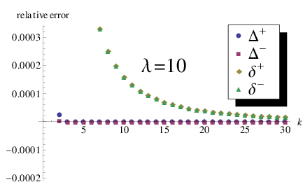
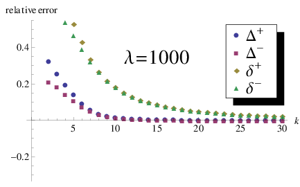
We first note, that the bare KS response does not have a spin-triplet component. Nevertheless, we take the bare KS resonances as a zeroth order guess for both, the spin-singlet and spin-triplet transitions. Therefore in general has a different relative error with respect to . This can be nicely seen in Fig. 5 in the difference between and for small values of . For large values of these differences as well as the relative error of the different approximations becomes small. For the bare KS resonance frequencies this can be explained by the fact, that the higher lying states are dominated by the kinetic energy and are less influenced by the interaction. On the other hand, since the SPA corresponds to the first term in a Laurent expansion with respect to [23], it becomes more accurate when the bare KS excitation energy is closer to the true resonance frequency. Hence the SPA inherits the high behaviour of the bare KS values. For the lower lying states we find that the SPA usually strongly improves upon the bare KS resonances (see Figs. 4 and 5). In our example the singly-excited states are well-separated from the doubly-excited states. In this case the SPA describes well the singly-excited states.
The adiabatic approximations based on LDA and the exchange-only kernel do not generate new poles and, not surprisingly, fail to describe the doubly-excited states of the system. In order to describe doubly-excited states a frequency-dependent xc kernel is required. We are not aware of any existing simple approximation for a memory kernel that would be able to reproduce the doubly-excited states of our model system. Some approximate kernels exist based on electron gas models, but such kernels would lead to artificial complex excitation energies. In any case, our exact expression for the xc kernel will serve as a useful benchmark to study future density functionals.
IV Outlook
In this work we have presented analytical expressions of exact density-functionals with initial-state dependence and memory. The functionals were used to give explicit examples of the otherwise very abstract concepts of the xc potential and the KS construction. We demonstrated how one can calculate the exact xc potential for an interacting model system and how one can construct the corresponding exact, frequency-dependent xc kernel. We have then shown how these analytical examples can be used to investigate the basic properties of time-dependent density-functionals and to test approximations.
These results will help to understand the properties of time-dependent density-functionals in more detail. For instance, they have already been used to investigate the Floquet-approach to TDDFT [24]. Further, these exact functionals show how initial-state dependence and memory have to be incorporated into more accurate functional approximations. As such one can employ these exact expressions as benchmarks for the development of new and more reliable functional approximations in TDDFT.
Acknowledgements.
We thank E. Räsänen, N.T. Maitra and K. Burke for valuable comments. M.R. acknowledges financial support by the Erwin Schrödinger Fellowship J 3016-N16 of the FWF (Austrian Science Fund). S.E.B.N. acknowledges support from the Lundbeck Foundation and from a grant to prof. Jeppe Olsen from the Danish Research Council. R.v.L. acknowledges the Academy of Finland for research funding.References
- [1] C. A. Ullrich, Time-Dependent Density-Functional Theory: Concepts and Applications (Oxford University Press, Oxford, 2012).
- [2] M. A. L. Marques, C. A. Ullrich, F. Nogueira, A. Rubio, K. Burke, and E. K. U. Gross, Time-Dependent Density Functional Theory (Springer, Heidelberg, 2012).
- [3] E. Runge and E. K. U. Gross, Phys. Rev. Lett. 52, 997 (1984), URL http://link.aps.org/doi/10.1103/PhysRevLett.52.997.
- [4] M. Ruggenthaler and R. van Leeuwen, Europhys. Lett. 95, 13001 (2011), URL http://stacks.iop.org/0295-5075/95/i=1/a=13001.
- [5] M. Ruggenthaler, K. J. H. Giesbertz, M. Penz, and R. van Leeuwen, Phys. Rev. A 85, 052504 (2012), URL http://link.aps.org/doi/10.1103/PhysRevA.85.052504.
- [6] I. D’Amico and G. Vignale, Phys. Rev. B 59, 7876 (1999), URL http://link.aps.org/doi/10.1103/PhysRevB.59.7876.
- [7] N. T. Maitra and K. Burke, Phys. Rev. A 63, 042501 (2001), URL http://link.aps.org/doi/10.1103/PhysRevA.63.042501.
- [8] N. T. Maitra, I. Souza, and K. Burke, Phys. Rev. B 68, 045109 (2003), URL http://link.aps.org/doi/10.1103/PhysRevB.68.045109.
- [9] R. van Leeuwen, Phys. Rev. Lett. 82, 3863 (1999), URL http://link.aps.org/doi/10.1103/PhysRevLett.82.3863.
- [10] J. Schirmer and A. Dreuw, Phys. Rev. A 75, 022513 (2007), URL http://link.aps.org/doi/10.1103/PhysRevA.75.022513.
- [11] N. T. Maitra, R. van Leeuwen, and K. Burke, Phys. Rev. A 78, 056501 (2008), URL http://link.aps.org/doi/10.1103/PhysRevA.78.056501.
- [12] M. Abramowitz and I. Stegun, Handbook of Mathematical Functions (Dover Publications, New York, 1972).
- [13] G. F. Giuliani and G. Vignale, Quantum Theory of the Electron Liquid (Cambridge University Press, Cambridge, 2005).
- [14] M. Hellgren and E. K. U. Gross, Phys. Rev. A 85, 022514 (2012), URL http://link.aps.org/doi/10.1103/PhysRevA.85.022514.
- [15] E. K. U. Gross and W. Kohn, Phys. Rev. Lett. 55, 2850 (1985), URL http://link.aps.org/doi/10.1103/PhysRevLett.55.2850.
- [16] C. A. Ullrich, U. J. Gossmann, and E. K. U. Gross, Phys. Rev. Lett. 74, 872 (1995), URL http://link.aps.org/doi/10.1103/PhysRevLett.74.872.
- [17] G. Vignale and W. Kohn, Phys. Rev. Lett. 77, 2037 (1996), URL http://link.aps.org/doi/10.1103/PhysRevLett.77.2037.
- [18] F. Sottile, V. Olevano, and L. Reining, Phys. Rev. Lett. 91, 056402 (2003), URL http://link.aps.org/doi/10.1103/PhysRevLett.91.056402.
- [19] A. Görling, in Time-Dependent Density Functional Theory, Lect. Notes Phys. 706 (Springer, Heidelberg, 2006).
- [20] M. Hellgren and U. von Barth, J. Chem. Phys. 132, 044101 (pages 5) (2010), URL http://link.aip.org/link/?JCP/132/044101/1.
- [21] M. Hellgren and U. von Barth, J. Chem. Phys. 131, 044110 (pages 13) (2009), URL http://link.aip.org/link/?JCP/131/044110/1.
- [22] M. E. Casida, in Recent Advances in Density Functional Methods, Volume 1, Recent Advances in Computational Chemistry (World Scientific, Singapore, 1995).
- [23] M. Petersilka, U. J. Gossmann, and E. K. U. Gross, Phys. Rev. Lett. 76, 1212 (1996), URL http://link.aps.org/doi/10.1103/PhysRevLett.76.1212.
- [24] V. Kapoor, M. Ruggenthaler, and D. Bauer, Phys. Rev. A 87, 042521 (2013), URL http://link.aps.org/doi/10.1103/PhysRevA.87.042521.