Slow Down & Sleep for Profit in
Online Deadline SchedulingThanks: This work was partially supported by the German Research Foundation (DFG) within the Collaborative Research Center “On-The-Fly Computing” (SFB 901) and by the Graduate School on Applied Network Science (GSANS).

Over the last decade, energy usage of data centers and computers in general has become a major concern. There are various reasons for this development: the ubiquity of technical systems, the rise of mobile computing, as well as a growing ecological awareness. Also from an economical viewpoint, energy usage can no longer be ignored. Energy costs for both the actual computation and the cooling have become the decisive cost factor in today’s data centers (see, e.g., [10]). In combination with improvements on the technical level, algorithmic research has great potential to reduce energy consumption. [2] gives a good insight on the role of algorithms to fully exploit the energy-saving mechanisms of modern systems. Two of the most prominent techniques for power saving are dynamic speed scaling and power-down. The former allows a system to save energy by adapting the processor’s speed to the current system load, while the latter can be used to transition into a sleep mode to conserve energy. There is an extensive body of literature on both techniques (see below). From an algorithmic viewpoint, the most challenging aspect in the design of scheduling strategies is to handle the lack of knowledge about the future: should we use a high speed to free resources in anticipation of new jobs or enter sleep mode in the hope that no new jobs arrive in the near future?

Given that profitability is a driving force for most modern systems and that energy consumption has gained such a high significance, it seems natural to take this relation explicitly into account. [16] consider a scheduling model that does so by introducing job values. Their scheduler controls energy usage via speed scaling and is allowed to reject jobs if their values seem too low compared to their foreseeable energy requirements. The objective is to maximize the profit, which is modeled as the total value of finished jobs minus the invested energy. Our work is based on a result by [12]. We enhance their model by combining speed scaling and power-down mechanisms for energy management, which not only introduces non-trivial difficulties to overcome in the analysis, but proves to be inherently more complex compared to the original model insofar that classical algorithms can become arbitrarily bad.

We are given a speed-scalable processor that can be set to any speed $s\in[0,\infty)$. When running at speed $s$ its power consumption is $P_{\alpha,\beta}(s)=s^{\alpha}+\beta$ with $\alpha\geq 2$ and $\beta\geq 0$. If $s(t)$ denotes the processor speed at time $t$, the total power consumption is $\int_{0}^{\infty}P_{\alpha,\beta}(s(t))\dif{t}$. We can suspend the processor into a sleep state to save energy. In this state, it cannot process any jobs and has a power consumption of zero. Though entering the sleep state is for free, waking up needs a fixed transition energy $\gamma\geq 0$. Over time, $n$ jobs $J=\left\{1,2,\ldots,n\right\}$ are released. Each job $j$ appears at its release time $r_{j}$ and has a deadline $d_{j}$, a (non-negative) value $v_{j}$, and requires a certain amount $w_{j}$ of work. The processor can process at most one job at a time. Preemption is allowed, i.e., jobs may be paused at any time and continued later on. If $I$ denotes the period of time (not necessarily an interval) when $j$ is scheduled, the amount of work processed is $\int_{I}s(t)\dif{t}$. A job is finished if $\int_{I}s(t)\dif{t}\geq w_{j}$. Jobs not finished until their deadline cause a cost equal to their value. We call such jobs rejected. A schedule $S$ specifies for any time $t$ the processor’s state (asleep or awake), the currently processed job (if the processor is awake), and sets the speed $s(t)$. W.l.o.g. we assume $s(t)=0$ when no job is being processed. Initially, the processor is assumed to be asleep. Whenever it is neither sleeping nor working we say it is idle. A schedule’s cost is the invested energy (for awaking from sleep, idling, and working on jobs) plus the loss due to rejected jobs. Let $m$ denote the number of sleep intervals, $l$ the total length of idle intervals, and $\mathcal{I}_{\text{work}}$ the collection of all working intervals (i.e., times when $s(t)>0$). Then, the schedule’s sleeping energy is $E^{S}_{\text{sleep}}:=(m-1)\gamma$, its idling energy is $E^{S}_{\text{idle}}:=l\beta$, and its working energy is $E^{S}_{\text{work}}:=\int_{\mathcal{I}_{\text{work}}}P_{\alpha,\beta}(s(t))\dif{t}$. We use $V^{S}_{\text{rej}}$ to denote the total value of rejected jobs. Now, the cost of schedule $S$ is

We seek online strategies yielding a provably good schedule. More formally, we measure the quality of online strategies by their competitive factor: For an online algorithm $A$ and a problem instance $I$ let $A(I)$ denote the resulting schedule and $O(I)$ an optimal schedule for $I$. Then, $A$ is said to be $c$-competitive if $\sup_{I}\frac{\operatorname{cost}(A(I))}{\operatorname{cost}(O(I))}\leq c$.

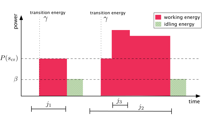
We define the system energy $E^{S}_{\text{sys}}$ of a schedule to be the energy needed to hold the system awake (whilst idling and working). That is, if $S$ is awake for a total of $x$ time units, $E^{S}_{\text{sys}}=x\beta$. Note that $E^{S}_{\text{sys}}\leq E^{S}_{\text{idle}}+E^{S}_{\text{work}}$. The critical speed of the power function is defined as $s_{\text{cr}}:=\arg\min_{s\geq 0}\nicefrac{{P_{\alpha,\beta}(s)}}{{s}}$ (cf. also [15, 14]). If job $j$ is processed at constant speed $s$ its energy usage is $w_{j}\cdot\nicefrac{{P_{\alpha,\beta}(s)}}{{s}}$. Thus, assuming that $j$ is the only job in the system and ignoring its deadline, $s_{\text{cr}}$ is the energy-optimal speed to process $j$. One can easily check that $s_{\text{cr}}^{\alpha}=\frac{\beta}{\alpha-1}$. Given a job $j$, let $\delta_{j}:=\nicefrac{{v_{j}}}{{w_{j}}}$ denote the job’s value density. Following [12] and [16], we define the profitable speed $s_{j,\text{p}}$ of job $j$ to be the maximum speed for which its processing may be profitable. More formally, $s_{j,\text{p}}:=\max\left\{s\geq 0\;\middle|\;w_{j}\cdot\nicefrac{{P_{\alpha,0}(s)}}{{s}}\leq v_{j}\right\}$. Note that the definition is with respect to $P_{\alpha,0}$, i.e., it ignores the system energy. The profitable speed can be more explicitly characterized by $s_{j,\text{p}}^{\alpha-1}=\delta_{j}$. It is easy to see that a schedule that processes $j$ at average speed faster than $s_{j,\text{p}}$ cannot be optimal: rejecting $j$ and idling during the former execution phase would be more profitable. See Figure 1 for an illustration of these notions.

This section considers a class of simple, deterministic online algorithms that we call rejection-oblivious. When a job arrives, a rejection-oblivious algorithm decides whether to accept or reject the job. This decision is based solely on the processor’s current state (sleeping, idling, working), its current workload, and the job’s properties. Especially it does not take former decisions into account. An example for such an algorithm is $PS(c)$ in [12]. For a suitable parameter $c$, it is $\alpha^{\alpha}+2e\alpha$-competitive in a model without sleep state. In this section we show that in our model (i.e., with a sleep state) no rejection-oblivious algorithm can be competitive. More exactly, the competitiveness of any such algorithm can become arbitrarily large. We identify the jobs’ value density as a crucial parameter for the competitiveness of these algorithms.

In the following, we use $A$ to refer to both our algorithm and the schedule it produces; which is meant should be clear from the context. As most algorithms in this area (see, e.g., [15, 6, 12, 14, 4]), $A$ relies heavily on the good structural properties of OA and its wide applicability to variants of the original energy-oriented scheduling model of [17]. It essentially consists of two components, the rejection policy and the scheduling policy. The rejection policy decides which jobs to accept or reject, while the scheduling policy ensures that all accepted jobs are finished until their deadline. Our rejection policy is an extension of the one used by the algorithm PS in [12]. It ensures that we process only jobs that have a reasonable high value (value $>$ planned energy investment) and that we do not awake from sleep for very cheap jobs. The scheduling policy controls the speed, the job assignment, and the current mode of the processor. It is a straightforward adaption of the algorithm used in [14]. However, its analysis proves to be more involved because we have to take into account its interaction with the rejection policy and that the job sets scheduled by the optimal algorithm and $A$ may be quite different.

The following description assumes a continuous recomputation of the current OA schedule. See Listing 1 for the corresponding pseudocode. It is straightforward to implement $A$ such that the planned schedule is recomputed only when new jobs arrive.

References

- [1] Susanne Albers “Algorithms for Dynamic Speed Scaling” In Proc. of the 28th International Symp. on Theoretical Aspects of Computer Science (STACS) Schloss Dagstuhl, 2011, pp. 1–11 DOI: 10.4230/LIPIcs.STACS.2011.1
- [2] Susanne Albers “Energy-Efficient Algorithms” In Comm. of the ACM 53.5 ACM, 2010, pp. 86–96 DOI: 10.1145/1735223.1735245
- [3] Susanne Albers and Antonios Antoniadis “Race to Idle: New Algorithms for Speed Scaling with a Sleep State” In Proceedings of the 23rd Symposium on Discrete Algorithms (SODA), 2012
- [4] Susanne Albers, Antonios Antoniadis and Gero Greiner “On Multi-Processor Speed Scaling with Migration” In Proceedings of the 23rd ACM Symposium on Parallelism in Algorithms and Architectures (SPAA) ACM, 2011, pp. 279–288 DOI: 10.1145/1989493.1989539
- [5] Nikhil Bansal, Tracy Kimbrel and Kirk Pruhs “Speed Scaling to Manage Energy and Temperature” In Journal of the ACM 54.1 ACM, 2007, pp. 1–39 DOI: 10.1145/1206035.1206038
- [6] Nikhil Bansal, Ho-Leung Chan, Kirk Pruhs and Dmitriy Katz “Improved Bounds for Speed Scaling in Devices Obeying the Cube-Root Rule” In Proceedings of the 36th International Colloquium on Automata, Languages and Programming (ICALP) Springer, 2009, pp. 144–155
- [7] Nikhil Bansal, Ho-Leung Chan, Tak-Wah Lam and Lap-Kei Lee “Scheduling for Speed Bounded Processors” In Proceedings of the 35th Intl. Colloq. on Automata, Languages and Programming (ICALP) Springer, 2008, pp. 409–420 DOI: 10.1007/978-3-540-70575-8˙34
- [8] Philippe Baptiste “Scheduling Unit Tasks to Minimize the Number of Idle Periods: A Polynomial Time Algorithm for Offline Dynamic Power Management” In Proceedings of the 17th Annual ACM-SIAM Symposium on Discrete Algorithm (SODA) ACM, 2006, pp. 364–367 DOI: 10.1145/1109557.1109598
- [9] Philippe Baptiste, Marek Chrobak and Christoph D“”urr “Polynomial Time Algorithms for Minimum Energy Scheduling” In Proceedings of the 15th Annual European Symposium on Algorithms (ESA) Springer, 2007, pp. 136–150 DOI: 10.1007/978-3-540-75520-3˙14
- [10] Luiz˜Andr“’e Barroso and Urs H“”olzle “The Case for Energy-Proportional Computing” In Computer 40.12 IEEE, 2007, pp. 33–37
- [11] S. Baruah, G. Koren, B. Mishra, A. Raghunathan, L. Rosier and D. Shasha “On-line Scheduling in the Presence of Overload” In Proc. of the 32nd Symp. on Foundations of Computer Science (FOCS), 1991, pp. 100–110 DOI: 10.1109/SFCS.1991.185354
- [12] Ho-Leung Chan, Tak-Wah Lam and Rongbin Li “Tradeoff between Energy and Throughput for Online Deadline Scheduling” In Proc. of the 8th Intl. Workshop on Approximation and Online Algorithms (WAOA) Springer, 2010, pp. 59–70 DOI: 10.1007/978-3-642-18318-8˙6
- [13] Ho-Leung Chan, Wun-Tat Chan, Tak-Wah Lam, Lap-Kei Lee, Kin-Sum Mak and Prudence W.˜H. Wong “Energy Efficient Online Deadline Scheduling” In Proceedings of the 18th Symposium on Discrete Algorithms (SODA) SIAM, 2007, pp. 795–804
- [14] Xin Han, Tak-Wah Lam, Lap-Kei Lee, Isaac K.˜K. To and Prudence W.˜H. Wong “Deadline Scheduling and Power Management for Speed Bounded Processors” In Theoretical Computer Science 411.40–42 Elsevier, 2010, pp. 3587–3600 DOI: 10.1016/j.tcs.2010.05.035
- [15] Sandy Irani, Sandeep Shukla and Rajesh Gupta “Algorithms for Power Savings” In ACM Transactions on Algorithms 3.4 ACM, 2007 DOI: 10.1145/1290672.1290678
- [16] Kirk Pruhs and Cliff Stein “How to Schedule When You Have to Buy Your Energy” In Proc. of the 13th/14th Workshop on Approximation Algorithms for Comb. Optimization Problems/Randomization and Computation (APPROX/RANDOM) Springer, 2010, pp. 352–365 DOI: 10.1007/978-3-642-15369-3˙27
- [17] Frances˜Foong Yao, Alan˜J. Demers and Scott Shenker “A Scheduling Model for Reduced CPU Energy” In Proceedings of the 36th Annual Symposium on Foundations of Computer Science (FOCS), 1995, pp. 374–382