Frequency-dependent fitness induces multistability in coevolutionary dynamics

Selection, random genetic drift and mutations are the processes underlying Darwinian evolution. For a long time population geneticists have analyzed the dynamics in the simplest setting consisting of two genotypes evolving under these processes [1]. In those studies, a genotype represents an individual’s genetic makeup, completely determining all relevant properties of the individual. A key concept is the so-called fitness of a genotype which represents the selection pressure for the individuals. The fitness defines the expected number of offspring an individual will produce. Thus, selection acts on fitness differences preferring individuals with higher fitness over individuals with lower fitness. Usually it is assumed that individuals have fixed fitnesses defined by their genotype alone [3, 1, 2]. Yet, experimental studies have revealed that many natural systems exhibit frequency-dependent selection [6, 4, 5], which means that an individual’s fitness not only depends on its genotype, but also on its interactions with other individuals and hence on the frequency of the different genotypes in the population. Although such frequency-dependent selection had already been studied early by Crow and Kimura [3], only recently has it received more attention [11, 12, 8, 13, 7, 9, 10, 14]. In these theoretical and computational studies, individuals’ interactions are represented by interaction matrices from game theory. This leads to a frequency dependence where the fitness depends directly on the interaction parameters in a linear way. However, fitness may depend on many diverse factors such as cooperation (i.e. individuals acting together to increase their fitness [12, 13]) and resource competition, so that certain systems may exhibit frequency-dependent fitness that is nonlinear. For example, in experiments certain hermaphrodites exhibit such nonlinear fitness-dependence [6]. To the best of our knowledge the impact of such nonlinear dependencies on coevolutionary dynamics has not been investigated theoretically.

In this article we show that nonlinear frequency dependence [15, 6] may induce new stable configurations of the evolutionary dynamics. Furthermore, we study the impact of asymmetric mutation probabilities on the dynamics [17, 16], which was also neglected in most models until now [13, 7, 9, 14]. As in previous works on coevolutionary dynamics we base our work on the Moran process in a non-spatial environment which is a well established model to study evolutionary dynamics and was already used in many applications [18]. The Moran process is a stochastic birth-death process which keeps the population size constant [19]. Therefore, in a two-genotype model the system becomes effectively one-dimensional, so that the dynamics may be described by a one-dimensional Markov chain with transition rates defined by the Moran process. We derive the stationary probability distribution of the system dynamics via its Fokker-Planck equation [20]. Sharp maxima of the distribution reveal metastable points of the dynamics and a multitude of such maxima lead to stochastic switching dynamics between multiple stable points.

The article is structured as follows. In Section II we introduce the model details and in Section III we derive the Fokker-Planck equation describing the probabilistic dynamics of the population. Using this equation we derive the stationary probability distribution that describes the long-time behavior of the system. In Section IV we analyze this probability distribution, which yields information about the impact of nonlinear frequency-dependent selection and of different mutation probabilities on the coevolutionary dynamics. In Section V we give a summary and discuss our results.

Consider a population of $N$ individuals evolving in a non-spatial environment, meaning that the population is well-mixed so that each individual interacts with all other individuals at all times. In this population the individuals may assume one out of two genotypes $A$ and $B$. The population sizes $k_{A}$ and $k_{B}$ ($k_{A}+k_{B}=N$) evolve according to the time-continuous Moran process described in the following, cf. [19]. The number of individuals $k_{A}$ of genotype $A$ completely determines the state of the system as $k_{B}=N-k_{A}$. At all times the interactions of the individuals determine the actual (frequency-dependent) fitness, so that an individual’s fitness of genotype $A$ or $B$ is defined by a fitness function $f_{A}(k_{A})$ or $f_{B}(k_{A})$ respectively. The fitness functions $f_{A}(k_{A})$ and $f_{B}(k_{A})$ may be any functions with the only condition that $f_{i}(k_{A})\geq 0$ for all $k_{A}\in[0,N]$ as negative fitness is not defined. At rate $f_{A}(k_{A})k_{A}$ an individual of type $A$ produces an identical offspring which may mutate to genotype $B$ with probability $\mu_{AB}$. This applies analogously to genotype $B$. Then one individual of the population is chosen randomly to die, so that the population size $N$ stays constant and the variables $k_{i}$ change maximally by $1$. This is the so-called Moran process which was originally introduced for a population of two genotypes with fixed fitnesses and no mutations occurring, cf. [19]. However, this process is easily generalizable to more genotypes and frequency-dependent selection in the way described above, cf. [11, 21].

Note that in our model the rate of reproduction of e.g. type $A$ is directly determined by the term $k_{A}f_{A}(k_{A})$ as e.g. in [22]. In other models the fitness is first normalized so that the rate of reproduction is given by $k_{A}f_{A}(k_{A})/\overline{f}(k_{A})$ [13], where

$$\overline{f}(k_{A})=\frac{1}{N}[k_{A}f_{A}(k_{A})+(N-k_{A})f_{B}(k_{A})]$$

(1)

is the population’s mean fitness. While in both of these models the events occur with the same probability, the times between the events differ by a common factor determined by the mean fitness (1). Thus, these models exhibit a quantitatively different time course, but the same event sequences.

Until now, usually linear functions have been considered for $f_{i}(k_{A})$. However, in many applications nonlinear functions seem more appropriate [15, 6]. For example, cooperation effects in game theory induce functions linearly increasing in $k_{A}$, so that $f_{A}(k_{A})=1+a\cdot k_{A}$ [11, 13]. This would mean that fitness increases infinitely with the population size of genotype $A$. Yet, in any habitat there is only a limited amount of resources available for living. Therefore, fitness should decline when the population of one genotype becomes too large as all of the individuals will compete for the same resources. We conclude that a fitness function including these two effects has to contain a nonlinear factor, e.g.

$$f_{A}(k_{A})=1+a\cdot k_{A}-b\cdot k_{A}^{2}$$

(2)

where $a>0$ and $b>0$. Here we choose a quadratic nonlinear factor as a simple example. Naturally, all other nonlinear functions could be applicable as well.

Note that linearly increasing fitness functions such as $f_{A}(k_{A})=1+a\cdot k_{A}$ and $f_{B}(k_{A})=1+b\cdot k_{A}$ lead to quadratic relations for the mean fitness $\overline{f}(k_{A})$ (see equation (1)) of the population which becomes

$$\overline{f}(k_{A})=1+bk_{A}+(a-b)\frac{k_{A}^{2}}{N}.$$

(3)

The quadratic factor originates from the fact that the linear fitness function in (1) is multiplied by the number of individuals leading to a quadratic dependence on $k_{A}$, e.g. $k_{A}f_{A}(k_{A})=k_{A}(1+ak_{A})=k_{A}+ak_{A}^{2}$. This factor enters the replicator equation in evolutionary game theory, thus leading to a quadratic fitness dependence in standard game theoretic problems [11, 22]. However, this does not imply nonlinear interactions and thus fitness effects such as presented in equation (2). Therefore, the fitness functions that can be generated by evolutionary game theory are a special case of the functions that occur in the theory presented here. Fitness functions as for example presented in equation (2) will – as we show in this article – lead to dynamics with more complex stability properties.

Usually, when analyzing the dynamics of such a model system as described above, it was assumed either that no mutations occur at all ($\mu_{ij}=0$) [19, 11, 10] or that the mutation probabilities are equal ($\mu_{AB}=\mu_{BA}$) [21, 13, 14]. However, usually mutation probabilities can be highly diverse [17, 16]. This has been considered in some examples [3], but until now the effect of different mutation probabilities in the introduced model system has not been studied systematically. Here, we explicitly study the effects caused by asymmetric mutation rates (see e.g. figure 2).

In the following we assume the fitness of the individuals to be given by

$$f_{A}(k)=1+g_{A}(k)$$

(4)

and

$$f_{B}(k)=1+g_{B}(k)$$

(5)

with the interaction functions $g_{A}>-1$ and $g_{B}>-1$. The model system is effectively one-dimensional with the variable $k\equiv k_{A}=N-k_{B}$ completely describing the system state [12]. At each event $k$ may change by at most $\pm 1$ depending only on the actual state of the system, so that the dynamics are Markovian. Let the transition $k\rightarrow k+1$ occur with the rate $r_{k}^{+}$. Then this rate is determined by the fitnesses and mutation probabilities in the following way:

• •

  Each individual in the population receives offspring with rate $f_{j}(k)$ with $j\in\{A,B\}$. This means that genotype $A$ receives one offspring with rate $k\cdot f_{A}(k)$.

• •

  Such an offspring increases the population $A$ with probability $1-\mu_{AB}$, and population $B$ in case it mutates with probability $\mu_{AB}$.

• •

  One individuum is chosen uniformly to die belonging to genotype $B$ with probability $(N-k)/(N+1)$.

• •

  Equivalently the number of individuals of genotype $A$ can increase if genotype $B$ receives one offspring, which mutates to genotype $A$ with probability $\mu_{BA}$, and one individuum of $B$ is chosen to die.

Taken these processes together the transition rate for $k\rightarrow k+1$ is

$$r_{k}^{+}=(1-\mu_{AB})kf_{A}(k)\cdot\frac{N-k}{N+1}+\mu_{BA}(N-k)f_{B}(k)\cdot\frac{N-k}{N+1}.$$

(6)

Decreasing $k$ to $k-1$ is equivalent to increasing the number of individuals of genotype $B$, so that the transition rate

$$r_{k}^{-}=(1-\mu_{BA})(N-k)f_{B}(k)\cdot\frac{k}{N+1}+\mu_{AB}kf_{A}(k)\cdot\frac{k}{N+1}$$

(7)

is obtained analogously. The master equation of the Markov chain is then given by

$$\frac{dp_{k}(t)}{dt}=r_{k-1}^{+}p_{k-1}(t)-(r_{k}^{-}+r_{k}^{+})p_{k}(t)+r_{k+1}^{-}p_{k+1}(t)\quad k\in\{0,N\}$$

(8)

where we define $r_{-1}^{+}=r_{N+1}^{-}=0$. As also $r_{0}^{-}=r_{N}^{+}=0$, the system has reflective boundaries at $k=0$ and $k=N$. If $\mu_{AB}=0$ ($\mu_{BA}=0$) then $k_{A}=N$ ($k_{A}=0$) is an absorbing state of the dynamics.

It is possible to derive the exact solution to such an equation similarly to the derivations in [23] which we do in Appendix B. However, the obtained solutions are not very explicit and their implications are hard to grasp. It is thus more useful to advance to the Fokker-Planck equation [20] describing the system in the limit of large $N$. As previous works have shown, this approximation already leads to very good results for moderate population sizes of $N<1000$, cf. [13]. We use the transformation

	$\displaystyle x=\frac{k}{N}\in[0,1],\qquad s=\frac{t}{N},\qquad\tilde{\mu}_{ij}=\mu_{ij}\cdot N,$		(9)
	$\displaystyle\rho(x,s)=p_{xN}(sN)N,\qquad\tilde{g}_{j}(x)=g_{j}(xN)\cdot N$		(10)

yielding the Fokker-Planck equation. The scaling factors are derived in Appendix A where the derivation of the Fokker-Planck equation in the scaling limit $N\rightarrow\infty$ is shown in detail (Equation (31)). This leads to

$$\frac{d\rho(x,s)}{ds}=-\frac{\partial}{\partial x}\Big[\left(\tilde{\mu}(1-2x)+\left[\tilde{g}_{A}(x)-\tilde{g}_{B}(x)\right]x(1-x)-\Delta\tilde{\mu}\right)\rho(x,s)\Big]+\frac{\partial^{2}}{\partial x^{2}}\Big[x(1-x)\rho(x,s)\Big]$$

(11)

with the normalization condition

$$\int_{0}^{1}\rho(x,s)dx=1$$

(12)

for all $s\geq 0$. Here $\tilde{g}_{A}=Ng_{A}(Nx)$ and $\tilde{g}_{B}=Ng_{B}(Nx)$ are the rescaled interaction functions defined in (10), $\tilde{\mu}=N(\mu_{AB}+\mu_{BA})/2$ is the rescaled mean mutation rate and $\Delta\tilde{\mu}=N(\mu_{AB}-\mu_{BA})/2$ is the rescaled mutation rate difference. These functions have to be rescaled to obtain a non-degenerate limit, the so-called weak selection regime.

Notice, that the drift term

$$D^{(1)}(x)=\tilde{\mu}(1-2x)+\left[\tilde{g}_{A}(x)-\tilde{g}_{B}(x)\right]x(1-x)-\Delta\tilde{\mu}$$

(13)

contains three different effects. The fitness difference at each point $x$ causes a selective drift, the mean mutation rate causes a drift directed to $x=1/2$ and the mutation rate difference causes a one-directional drift towards one of the boundaries $x=0$ or $x=1$. The diffusion term

$$D^{(2)}(x)=x(1-x)$$

(14)

reflects the undirected genetic drift.

If fitness differences are on a scale of $\mathcal{O}\left(N^{-1}\right)$, then mutation, selection and genetic drift all act on the same scale [24, 13]. Then the dynamics are characterized by an interplay of these different effects. On the other hand, in the strong selection regime – where fitness differences are on a scale $\mathcal{O}(1)$ – genetic drift becomes negligible and the dynamics in the bulk of the system become deterministic for large $N$ [25]. However, as the factor $x(1-x)$ vanishes for $x\rightarrow 0$ and $x\rightarrow 1$ the effects of mutations play an important role. Clearly, without mutations $x=0$ and $x=1$ are absorbing states, but even in the strong selection regime they become non-absorbing for any positive mutation rate. This is reflected in the form of the drift term $D^{(1)}(x)$, as only the factors reflecting mutations $\tilde{\mu}(1-2x)-\Delta\tilde{\mu}$ remain non-zero in the limits $x\rightarrow 0$ and $x\rightarrow 1$.

For a one-dimensional Fokker-Planck equation (11) the stationary distribution is [20]

$$\rho^{\ast}(x)=Ce^{-\Phi(x)}$$

(15)

with the potential

$$\Phi(x)=\ln\left(D^{(2)}(x)\right)-\int\frac{D^{(1)}(x)}{D^{(2)}(x)}dx$$

(16)

which is defined up to a constant irrelevant to our calculations as it is canceled by the normalization

$$C=\frac{1}{\int_{0}^{1}e^{-\Phi(x)}dx}.$$

(17)

Thus, we obtain

	$\displaystyle\Phi(x)$	$\displaystyle=$	$\displaystyle\ln\left(x(1-x)\right)-\int\left[\frac{\tilde{\mu}(1-2x)}{x(1-x)}+\tilde{g}_{A}(x)-\tilde{g}_{B}(x)-\frac{\Delta\tilde{\mu}}{x(1-x)}\right]dx$
		$\displaystyle=$	$\displaystyle\ln\left(x(1-x)\right)-\tilde{\mu}\ln(x(1-x))+\Delta\tilde{\mu}\ln\left[\frac{x}{1-x}\right]-\int\left[\tilde{g}_{A}(x)-\tilde{g}_{B}(x)\right]dx$

where we used

$$(1-2x)=\frac{\partial}{\partial x}[x(1-x)].$$

(18)

The stationary solution becomes

$$\rho^{\ast}(x)=C\left(x(1-x)\right)^{\tilde{\mu}-1}\left(\frac{x}{1-x}\right)^{-\Delta\tilde{\mu}}e^{\int\left[\tilde{g}_{A}(x)-\tilde{g}_{B}(x)\right]dx}$$

(19)

where the constant $C$ defined in (17) has to be calculated numerically for given parameters.

This stationary distribution contains contributions from the above mentioned four different effects:

1. 1.

   Genetic drift is reflected by $(x(1-x))^{-1}$ which diverges for $x\in\{0,1\}$ at the boundaries.

2. 2.

   The mean mutation rate $\tilde{\mu}>0$ causes the balancing term $(x(1-x))^{\tilde{\mu}}$.

3. 3.

   The asymmetry in the mutation probabilities causes the term $(x/(1-x))^{-\Delta\tilde{\mu}}$ which diverges at one boundary and vanishes at the other.

4. 4.

   All frequency-dependent selection effects are contained in the exponential factor $e^{\int\left[\tilde{g}_{A}(x)-\tilde{g}_{B}(x)\right]dx}$ which can take various shapes.

What are the possible shapes for the stationary distribution $\rho^{\ast}(x)$ in the form given by equation (19)? Until now, the term $(x/(1-x))^{-\Delta\tilde{\mu}}$ representing the asymmetric mutation probabilities has not been considered to our knowledge and the interaction functions $\tilde{g}_{A}(x)$ and $\tilde{g}_{B}(x)$ in the selection term were considered to be at most linear in $x$ [13]. We should therefore be interested in the effects of nonlinear interaction functions and asymmetric mutation rates.

Let us first analyze the dynamics for nonlinear interaction functions [15, 6] describing the effects of cooperation and limited resources as described by equation (2), so that

$$\tilde{g}_{A}(x)=N\left(a_{A}x-b_{A}x^{2}\right)\qquad\tilde{g}_{B}(x)=N\left(a_{B}(1-x)-b_{B}(1-x)^{2}\right).$$

(20)

Already with $\Delta\tilde{\mu}=0$ such interaction functions induce dynamics stochastically switching between three metastable points. An example is shown in Figure 1, where the theoretically calculated stationary distribution from equation (19) is shown together with data from simulations with a population of $N=1000$ individuals which is enough to obtain almost perfect fitting (cf. also Figure 4). The fitness functions (Figure 1b) both show at first an increase on increasing the number of individuals of genotype $A$ or $B$ from $0$ due to cooperation effects and then a strong decrease due to resource competion. As the resulting fitness functions are asymmetric, also the stationary distribution is asymmetric. There is a maximum at $x=0$ due to genetic drift. Selection drives the dynamics towards a metastable state at $x\approx 0.2$, because for $x<0.2$ genotype $A$ is fitter than $B$ thus increasing in frequency and for $x>0.2$ genotype $A$ is less fit than $B$ thus decreasing in frequency (cf. Figure 1b). The maximum of the stationary distribution is thus exactly at the point where $f_{A}(x)=f_{B}(x)$. For $x>0.7$ again genotype $A$ is fitter than $B$ and thus the dynamics are driven towards $x=1$ by selection as well as genetic drift. The mutational force induced by $\tilde{\mu}=0.5$ increases the height of the maximum at $x\approx 0.2$ driving the system away from the maxima at $x=0$ and $x=1$. So, in this example genetic drift, mutation and selection all significantly influence the dynamics.

Let us now study the influence of the mutation rates in detail. Interestingly, for asymmetric mutation rates ($\Delta\tilde{\mu}\neq 0$) the factor $(x/(1-x))^{-\Delta\tilde{\mu}}$ always diverges in the interval $[0,1]$. For $\Delta\tilde{\mu}>0$ it diverges for $x\rightarrow 0$, otherwise for $x\rightarrow 1$. This can cause the emergence of a maximum of the stationary distribution at $x=0$ (or resp. $x=1$). Figure 2 shows an example where due to asymmetric mutation rates a maximum occurs at $x=1$, when for $\Delta\tilde{\mu}=0$ there is an absolute minimum at $x=1$ as this stable state minimizes the population’s mean fitness. This means, that the system dynamics are mutation dominated near $x=1$. Furthermore, the maximum located at $x=0$ for $\Delta\tilde{\mu}=0$ is shifted for $\Delta\tilde{\mu}>0$ to values $x>0$ causing a minimum of the stationary distribution at $x=0$. Thus, in this example both selection and the asymmetry in mutation probabilities are the driving forces of the system’s dynamics.

For low mutation rates the population has a high tendency to become dominated by one of the two genotypes for long times which is illustrated in Figure 3a. Thus, the dynamics stay close to the edges $x=0$ or $x=1$ waiting for one of the few mutations to occur. For low overall mutation rates differences in the mutation rates have only weak effects. High mutation rates cause the population to be drawn towards a mixture of both genotypes ($x\approx 0.5$). Even more, for high mutation rates the differences in the mutation rates $\Delta\tilde{\mu}$ can have an important influence on the dynamics. For instance Figure 3b illustrates a shift of an existing stable point, which completely vanishes for high $\Delta\tilde{\mu}$. We conclude that asymmetric mutation rates can cause the emergence of new stable states (as in Figure 2), the disappearance of existing ones (as in Figure 3), and shift existing stable states to new positions.

As we saw above, the fit of the theoretically calculated stationary distribution to simulation data is almost perfect for weak selection, i.e. the maximal fitness difference satisfies $\Delta f_{\text{max}}\ll 1$, cf. e.g. [13]. To quantify the quality of the fit we measured the stationary distribution with the same parameters as above for different population sizes $N$. This is shown in Figure 4 demonstrating that for increasing $N$ the data gets ever closer to the theoretically obtained distribution. For this we define the empirical distribution

$$\pi_{k}:=\frac{1}{T_{\text{meas}}}\sum_{t=0}^{T_{\text{meas}}}\delta(X_{t+T_{\text{mix}}},k)$$

(21)

where $(X_{t}:\,t\geq 0)$ is the discrete process defined in equation (8). $T_{\text{mix}}$ is a time large enough for the process to reach stationarity and depends on the system size, as does the measurement time $T_{\text{meas}}$ which is specified in Figure 4. Using this definition we quantify the quality of the fit using the distance measure

$$\overline{d}:=\frac{1}{N}\sum_{k=1}^{N-1}\left|\pi_{k}-\int_{k/N-1/2N}^{k/N+1/2N}\rho^{\ast}(x)dx\right|$$

(22)

which takes the mean distance of the measured empirical distribution $\pi_{k}$ from the theoretical distribution for every point except $k=0$ and $k=N$ where the density $\rho^{\ast}(x)$ diverges. Here, the the theoretical distribution is calculated by integrating the theoretical density over bins of the size $1/N$ around the points $k/N$. Figure 4b shows that the mean distance $\overline{d}$ decays with increasing $N$.

The decay of this quantity is dominated by the slow convergence at the domain boundaries $k=0$ and $k=N$. Therefore, we additionally defined the maximum distance measure

$$d_{\text{max}}:=\max_{k\in[1,N-1]}\left\{\left|\pi_{k}-\int_{k/N-1/2N}^{k/N+1/2N}\rho^{\ast}(x)dx\right|\right\}$$

(23)

which gives the maximum distance between the measured probability distribution from the theoretical distribution for all points except $k=0$ and $k=N$ due to the same argument as above. Figure 4b shows that the maximum distance $d_{\text{max}}$ decreases with increasing $N$, however slower than the mean distance $\overline{d}$ due to the divergence of $\rho(x)$ at the boundaries. Altogether we conclude, that the theoretical curve fits the data very well already for $N\succsim 1000$. However, near the domain boundaries special care has to be taken, as divergences of the theoretical curve lead to larger deviations.

Furthermore, as the Fokker-Planck approximation only holds for weak selection we study the quality of the solution obtained throught the Fokker-Planck equation in dependence of the selection strength. For this we introduce a scaling factor $\xi$ to the interaction functions, so that they become

$$\tilde{g}_{A}(x)=\xi N\left(a_{A}x-b_{A}x^{2}\right)\qquad\tilde{g}_{B}(x)=\xi N\left(a_{B}(1-x)-b_{B}(1-x)^{2}\right).$$

(24)

We find that the stationary solution of the Fokker-Planck equation well approximates the solution of the Master equation

$$p_{k}^{\ast}=\frac{\prod_{j=0}^{k-1}\frac{r_{j}^{+}}{r_{j+1}^{-}}}{\sum_{l=0}^{N}\prod_{j=0}^{l-1}\frac{r_{j}^{+}}{r_{j+1}^{-}}}$$

(25)

for selection strengths up to $\xi$ of the order of 1 (cf. Figure 5 ). We derive the solution (25) of the Master equation in Appendix B. Note that for the derivation of this solution no approximation is necessary and it hence fits data from simulations perfectly up to an error due to finite sampling in simulations. As Figure 5 illustrates, for strong selection $\xi\succsim 1$ the solution of the Fokker-Planck equation does not fit the exact solution of the Master equation perfectly, but still catches the overall trend of the dynamics. The error, quantified by the mean distance measure analogous to (22), increases with $\xi$ as a power law both in comparison with the solution from the Master equation and with data from simulations, cf. Figure 5d. All in all, for weak selection the Fokker-Planck approximation works well while for strong selection it does not perfectly predict the stationary distribution, but still reflects the overall trend of the dynamics. If this approximation is not satisfying, the direct solution (25) of the Master equation yields the exact distribution fitting the data for all selection strengths.

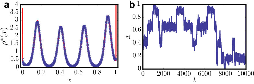
We have shown above that the dynamics of a two-genotype system can exhibit multiple stable points induced by nonlinear selection. Even more, there is no theoretical limit to the number of stable points in the system. Assume for example $\tilde{\mu}=1$ and $\Delta\tilde{\mu}=0$, so that mutation exactly balances genetic drift. Then, the stationary distribution (19) has a maximum at each point, where $\exp\left[\int\tilde{g}_{A}(x)-\tilde{g}_{B}(x)dx\right]$ has a maximum. Theoretically $\tilde{g}_{A}(x)$ and $\tilde{g}_{B}(x)$ can be any function with an arbitrary amount of extreme points in $[0,1]$, so that there is no limit to the stationary distribution’s number of maxima, if selection dominates the dynamics. However, for finite $N$ the number of possible maxima is naturally limited by $N/2$. Figure 6 shows an example, where we used periodic interaction functions

$$\tilde{g}_{A}(x)=\alpha\left(1+\sin(\beta x)\right)\text{ and }\tilde{g}_{B}(x)=\alpha\left(1+\cos(\beta x)\right).$$

(26)

Although this is not a realistic interaction function in most applications, it demonstrates what is theoretically possible in the introduced system.

In this article we analyzed a two-genotype system in a very general setting with (possibly) asymmetric mutation probabilities and nonlinear fitness functions [15, 6] in finite populations. The underlying Moran process is a well established model [1, 12, 13] to gain an understanding of the interplay of selection, mutation and genetic drift in evolutionary dynamics. However, the Moran process is studied mostly with symmetric mutation probabilities and at most linear interaction functions. We reasoned that neither need mutation probabilities be symmetric – as experiments have shown, that mutation probabilities are often asymmetric [16] – nor can all interaction effects be described by linear interaction functions. For example cooperation in game theory leads to an interaction function increasing linearly in the frequency of the cooperating genotype. Yet, in many applications also cooperators in the end compete for the same type of resource which is limited. Therefore, due to limited resources a population being too large cannot be sustained leading to a decrease in the fitness. There is no linear function that can reflect both of these effects at the same time.

We derived the Fokker-Planck equation describing the dynamics of the number of individuals $k$ of genotype $A$ in the limit of large population sizes $N$. We quantified the quality of the Fokker-Planck approach for an example (cf. Figure 4) where the difference of simulation data and theoretical solution became almost not detectable for population sizes larger than $N\succsim 1000$. Actually, if the system exhibits absorbing states then the Fokker-Planck method does not work to study the corresponding quasi-stationary distributions. Instead, WKB methods are more appropriate to describe the system dynamics as for example in [10], where fixation resulting from large fluctuations was studied. In our model system no such absorbing states exist, as long as the mutation rates are positive ($\mu_{ij}\neq 0$) and therefore the Fokker-Planck equation is appropriate to describe the system dynamics.

We identified the individual effects of selection, mean mutation rate and mutation difference as well as genetic drift and derived the stationary probability distribution as determined by the Fokker-Planck equation. Analyzing the distribution, we found that asymmetries in the mutation probabilities may not only induce the shifting of existing stable points of the dynamics to new positions, but also lead to the emergence of new stable points. Thus, a genotype that has a selective disadvantage can anyway have a stable dynamical state where its individuals dominate the population due to a higher mutational stability (see Figure 2). Further we found, that dynamic fitness leads to multiple stable points of the dynamics induced by selection and also genetic drift. We showed an example (Figure 1) where three stable points exist, two caused by selection and one by genetic drift.

We conclude that frequency-dependent fitness together with asymmetric mutation rates induces complex evolutionary dynamics, in particular if the interactions imply nonlinear fitness functions. Theoretically, there is no limit for the number of stable points that the dynamics can exhibit (see Figure 6). All in all, we interprete our results such that in real biological systems multiple metastable equilibria may exist, whenever species interact in a way complex enough to imply a fitness that nonlinearly depends on frequency. As a consequence, one species may exhibit a certain frequency for a long time before a sudden shift occurs and then a new frequency prevails. Such a change may thus occur even in the absence of changes of the environment; it may be induced as well by a stochastic switching from one metastable state to another due to complex inter-species interactions.

The Moran process is a standard tool to gain theoretical insights into experimental data [18]. Of course, we do not propose here that any experimental setup may be exactly described by the Moran process. However, we think that it should be feasible to develop an experiment where two different mutants evolve with asymmetric mutation rates. To find an experimental setup where the two genotypes also exhibit nonlinear fitness could however prove more difficult. Rather, our study is a theoretical study indicating that nonlinear fitness may be the cause of multible stable states when observed in experimental data.

For further studies on systems with more genotypes it should be useful to combine our considerations presented here with the work of Traulsen et al. [13], where an analysis of systems with more than two genotypes was carried out. Extending those results it may be possible to gain a better understanding of the effects of nonlinear interactions for many different genotypes. Also, it may be interesting to study the effects of changing interactions, where the interactions change according to the system dynamics [26]. Thus, our study might serve as a promising starting point to investigate how nonlinear frequency dependencies impact evolutionary dynamics in complex environments.

Acknowledgements

We thank Steven Strogatz for fruitful discussions during project initiation and Stefan Eule for helpful technical discussions. Stefan Grosskinsky acknowledges support by EPSRC, grant no. EP/E501311/1.

The master equation (8) may be transformed to a Fokker-Planck equation in the limit of large $N$ [20]. We introduce the transformation

$$x=\frac{k}{N}\qquad s=t\cdot F(N)\qquad\tilde{\mu}_{ij}=\mu_{ij}\cdot G(N)$$

(27)

together with the rescaled functions

$$\rho(x,s)=p_{Nx}(t)N\qquad\tilde{g}_{j}(x)=g_{j}(k)\cdot H(N).$$

(28)

We fix the scaling functions $F(N)$, $G(N)$ and $H(N)$ such that in the limit $N\rightarrow\infty$ all terms in equation (8) remain finite so that mutation, selection and genetic drift all act on the same scale. We further define

$$x_{-}=x-\frac{1}{N}\qquad x_{+}=1+\frac{1}{N}$$

(29)

and substituting all this into the master equation (8), we obtain

	$\displaystyle\frac{d\rho(x,s)}{ds}F(N)$	$\displaystyle=$	$\displaystyle\frac{N^{2}}{N+1}\left\{\left[(1-\mu_{AB})(1+g_{A}(x_{-}))x_{-}(1-x_{-})+\mu_{BA}(1+g_{B}(x_{-}))(1-x_{-})^{2}\right]\rho(x_{-},s)\right.$		(30)
			$\displaystyle\left[(1-\mu_{BA})(1+g_{B}(x_{+}))(1-x_{+})x_{+}+\mu_{AB}(1+g_{A}(x_{+}))x_{+}^{2}\right]\rho(x_{+},s)$
			$\displaystyle-\left[(1-\mu_{AB})(1+g_{A}(x))x(1-x)+\mu_{BA}(1+g_{B}(x))(1-x)^{2}\right.$
			$\displaystyle+\left.\left.(1-\mu_{BA})(1+g_{B}(x))x(1-x)+\mu_{AB}(1+g_{A}(x))x^{2}\right]\rho(x,s)\right\}$

We choose $F(N)=1/(N+1)$ and $G(N)=H(N)=N$ so that in the limit $N\rightarrow\infty$ the terms stay finite. Further we introduce the mean mutation rate $\tilde{\mu}=N(\mu_{AB}+\mu_{BA})/2$ and the mutation rate difference $\Delta\tilde{\mu}=N(\mu_{AB}-\mu_{BA})/2$. To not overload the notation we drop the time argument $s$ of $\rho(x,s)$ in the following calculation. This leads to

	$\displaystyle\frac{d\rho(x)}{ds}$	$\displaystyle=$	$\displaystyle N^{2}\left\{-2x(1-x)\rho(x)+x_{+}(1-x_{+})\rho(x_{+})+x_{-}(1-x_{-})\rho(x_{-})\right.$
			$\displaystyle+\left.\frac{\tilde{\mu}}{N}\left[-(1-2x)^{2}\rho(x)+\frac{1}{2}(1-2x_{+})^{2}\rho(x_{+})+\frac{1}{2}(1-2x_{-})^{2}\rho(x_{-})\right]\right\}$
			$\displaystyle+N\left\{\tilde{g}_{A}(x_{-})x_{-}(1-x_{-})\rho(x_{-})-\tilde{g}_{A}(x)x(1-x)\rho(x)+\tilde{g}_{B}(x_{+})x_{+}(1-x_{+})\rho(x_{+})-\tilde{g}_{B}(x)x(1-x)\rho(x)\right.$
			$\displaystyle+\frac{\tilde{\mu}}{2}\left[(1-2x_{-})\rho(x_{-})-(1-2x_{+})\rho(x_{+})\right]$
			$\displaystyle+\Delta\tilde{\mu}\left[x_{+}\rho(x_{+})-x\rho(x)-(1-x_{-})\rho(x_{-})+(1-x)\rho(x)\right]$
			$\displaystyle+\frac{\tilde{\mu}}{N}\left[\left(\tilde{g}_{A}(x_{+})x_{+}^{2}+\tilde{g}_{B}(x_{+})(x_{+}^{2}-x_{+})\right)\rho(x_{+})-\left(\tilde{g}_{A}(x)x^{2}+\tilde{g}_{B}(x)(x^{2}-x)\right)\rho(x)\right.$
			$\displaystyle+\left.\left(\tilde{g}_{A}(x_{-})(x_{-}^{2}-x_{-})+\tilde{g}_{B}(x_{-})(1-x_{-})^{2}\right)\rho(x_{-})-\left(\tilde{g}_{A}(x)(x^{2}-x)+\tilde{g}_{B}(x)(1-x)^{2}\right)\rho(x)\right]$
			$\displaystyle+\frac{\Delta\tilde{\mu}}{N}\left[\left(\tilde{g}_{A}(x_{+})x_{+}^{2}-\tilde{g}_{B}(x_{+})(x_{+}^{2}-x_{+})\right)\rho(x_{+})-\left(\tilde{g}_{A}(x)x^{2}-\tilde{g}_{B}(x)(x^{2}-x)\right)\rho(x)\right.$
			$\displaystyle+\left.\left.\left(\tilde{g}_{A}(x_{-})(x_{-}^{2}-x_{-})-\tilde{g}_{B}(x_{-})(1-x_{-})^{2}\right)\rho(x_{-})-\left(\tilde{g}_{A}(x)(x^{2}-x)-\tilde{g}_{B}(x)(1-x)^{2}\right)\rho(x)\right]\right\}$

In the limit $N\rightarrow\infty$ the different terms with $N^{2}$ in front become second order derivatives with respect to $x$, while the other terms become first order derivatives. The terms which have a $1/N$ factor vanish in the limit $N\rightarrow\infty$ and thus the above equation becomes

$$\frac{d\rho}{ds}=-\frac{\partial}{\partial x}\left[\tilde{\mu}(1-2x)\rho(x)+\left(\left[\tilde{g}_{A}(x)-\tilde{g}_{B}(x)\right]x(1-x)\rho(x)\right)-\Delta\tilde{\mu}\rho(x)\right]+\frac{\partial^{2}}{\partial x^{2}}\left[x(1-x)\rho(x)\right]$$

(31)

which is the Focker-Planck-Equation of the system.

We directly derive the stationary solution $p_{k}^{\ast}$ of the master equation (8) using the detailed balance equation

$$r_{k-1}^{+}p_{k-1}^{\ast}=r_{k}^{-}p_{k}^{\ast}$$

(32)

which applies to any chain with only nearest neighbour transitions [20], cf. also [23]. Thus, using the rewritten balance equation

$$p_{k}^{\ast}=\frac{r_{k-1}^{+}}{r_{k}^{-}}\cdot p_{k-1}^{\ast}$$

(33)

iteratively, we obtain

$$p_{k}^{\ast}=p_{0}^{\ast}\prod_{j=0}^{k-1}\frac{r_{j}^{+}}{r_{j+1}^{-}}.$$

(34)

Finally, we may use the normalization condition

$$\sum_{l=0}^{N}p_{l}^{\ast}=1$$

(35)

of the stationary distribution to eliminate the factor $p_{0}^{\ast}$. We then obtain the exact stationary solution of the master equation

$$p_{k}^{\ast}=\frac{\prod_{j=0}^{k-1}\frac{r_{j}^{+}}{r_{j+1}^{-}}}{\sum_{l=0}^{N}\prod_{j=0}^{l-1}\frac{r_{j}^{+}}{r_{j+1}^{-}}}$$

(36)

which can be evaluated numerically for any transition rates $r_{k}^{+}$ and $r_{k}^{-}$. For more details on the exact solution of the Master equation in the Moran process see for example the work by Claussen and Traulsen [23].

References

- [1] B. Drossel, Adv. Phys. 50, 209 (2001).
- [2] R. A. Blythe and A. J. McKane, J. Stat. Mech. P07018 (2007).
- [3] J. F. Crow and M. Kimura, An Introduction to Population Genetics Theory (Harper & Row Publishers, New York, USA, 1970).
- [4] P. E. Turner and L. Chao, Nature 398, 441-443 (1999).
- [5] J. Gore, H. Youk and A. van Oudenaarden, Nature 459, 253-256 (2009).
- [6] D. E. McCauley and M. T. Brock, Evolution 52, 30 (1998).
- [7] T. Antal, M. A. Nowak, and A. Traulsen, J. Theor. Biol. 257, 340 (2009a).
- [8] T. Antal and I. Scheuring, Bull. Math. Biol. 68, 1923 (2006).
- [9] T. Antal, A. Traulsen, H. Ohtsuki, C. E. Tarnita, and M. A. Nowak, J. Theor. Biol. 258, 614 (2009b).
- [10] M. Assaf and M. Mobilia, J. Stat. Mech. P09009 (2010).
- [11] C. Taylor, D. Fudenberg, A. Sasaki, and M. A. Nowak, Bull. Math. Biol. 66, 1621 (2004).
- [12] A. Traulsen, J. C. Claussen, and C. Hauert, Phys. Rev. Lett. 95, 238701 (2005).
- [13] A. Traulsen, J. C. Claussen, and C. Hauert, Phys. Rev. E 74, 011901 (2006).
- [14] B. Wu, C. S. Gokhale, L. Wang, and A. Traulsen, J. Math. Biol. 62, DOI 10.1007/s00285 (2011).
- [15] H.-J. Pohley and B. Thomas, Biosystems 16, 87 (1983).
- [16] R. Durett and D. Schmidt, Genetics 180, 1501 (2008).
- [17] A. Sasaki and M. A. Nowak, J. Theor. Biol. 224, 241 (2003).
- [18] S. Nee, Annu. Rev. Ecol. Evol. Syst. 37, 1-17 (2006).
- [19] P. A. P. Moran, The statistical processes of evolutionary theory (Clarendon Press, Oxford, UK, 1962).
- [20] H. Risken, The Fokker-Planck equation (Springer-Verlag, Berlin, Germany, 1989).
- [21] L. A. Imhof, D. Fudenberg, and M. A. Nowak, Proc. Natl. Acad. Sci. U.S.A. 102, 10797 (2005).
- [22] A. J. Bladon, T. Galla, and A. J. McKane, Phys. Rev. E 81, 066122 (2010).
- [23] J. C. Claussen and A. Traulsen, Phys. Rev. E 71, 025101(R) (2005).
- [24] T. Ohta, Proc. Natl. Acad. Sci. U.S.A. 99, 16134 (2002).
- [25] K. Jain and J. Krug, Genetics 175, 1275 (2007).
- [26] T. Gross and B. Blasius, J. R. Soc. Interface 5, 259 (2008).