Searching for axions and ALPs from string theory

We will consider here type IIB flux compactifications on Calabi-Yau orientifolds $X$ in the presence of space-time filling $D7$ branes and $O7$ planes. Below the Kaluza-Klein scale $M_{\rm KK}$, they lead to a low-energy $\mathcal{N}=1$ (supergravity) EFT in 4D. Their 4D closed string moduli, comprised by the axio-dilaton $S=e^{-\phi}+iC_{0}$, the complex structure moduli $U_{\alpha}$, $\alpha=1,...,h_{-}^{2,1}(X)$, and the Kähler moduli,

are obtained via the Kaluza-Klein reduction of the massless bosonic fields of the original 10D theory – the latter including, in the Ramond-Ramond sector, the forms $C_{0}$ and $C_{4}$, and, in the Neveu Schwarz-Neveu Schwarz sector, the dilaton $\phi$. Importantly, the number of Kähler moduli $T_{i}$ is determined by the topology of $X$, namely the number of inequivalent four-cycles $D_{i}$ of $X$ (we have specialised for convenience to orientifold projections such that $h^{1,1}_{-}=0\Rightarrow h^{1,1}_{+}=h^{1,1}$). Their imaginary parts $c_{i}$ have all the properties of axion-like fields, as we will see next.

As already mentioned, (a suitable extension of) the standard model is realised in such compactifications through (stacks of) space-time filling $D7$-branes wrapping some of the four-cycles $D_{i}$. At low energies, the dynamics of a $D7$-brane reduces to a $U(1)$ gauge theory that lives on its eight-dimensional world-volume. Moreover, $D7$-branes can be magnetised by turning on internal magnetic fluxes $\mathcal{F}$. Taking all these effects into account, the 4D low energy effective Lagrangian of the axion-like fields $c_{i}$, including the brane-localised $U(1)$ gauge bosons $A_{i}$, is obtained from the Kaluza-Klein reduction of the $D7$-brane action as follows [23, 24]:

where $M_{P}=(8\pi G_{N})^{-1/2}\simeq 2.4\cdot 10^{18}$ GeV is the reduced Planck mass, while the various other quantities in Eq. (8) are defined as follows:

• •

  The Kähler metric $K_{\alpha\beta}$, describing the kinetic mixing of the axion-like fields, is obtained via $\mathcal{K}_{\alpha\beta}\equiv\frac{\partial^{2}K}{\partial\tau_{\alpha}\partial\tau_{\beta}}$ from the Kähler potential, the latter taking, at tree-level, the following form:

  $$K_{\rm tree}=-2\ln\mathcal{V}-\ln\left(S+\bar{S}\right)-\ln\left(-i\int\limits_{X}\Omega\wedge\bar{\Omega}\right)\,.$$

  (9)

  It depends implicitly on the complex structure moduli via the holomorphic (3,0)-form $\Omega$ and on the Kähler moduli via the Calabi-Yau volume $\mathcal{V}$, measured by an Einstein frame metric $g^{\scriptscriptstyle E}_{\mu\nu}=e^{-\phi/2}\,g^{s}_{\mu\nu}$, and expressed in units of the string length $\ell_{s}=2\pi\sqrt{\alpha^{\prime}}$, in terms of its tension $\alpha^{\prime}$,

  $$\mathcal{V}=\frac{1}{6}\int_{X}J\wedge J\wedge J=\frac{1}{6}\,k_{\alpha\beta\gamma}t^{\alpha}t^{\beta}t^{\gamma}\,.$$

  (10)

  Here, the Kähler form $J$ has been expanded, in a basis $\{\hat{D}_{\alpha}\}_{\alpha=1}^{h^{1,1}}$ of $H^{1,1}(X,\mathbb{Z})$ of two-forms which are Poincaré dual to $D_{\alpha}$, as $J=t^{\alpha}\hat{D}_{\alpha}$, and we denoted the triple intersection numbers of $X$ by $k_{\alpha\beta\gamma}$. The volume, the Kähler form and ultimately the Kähler metric can then be obtained as a function of the $\tau_{\alpha}$ by inverting the following relations:

  $$\tau_{\alpha}=\frac{1}{2}\int_{X}\hat{D}_{\alpha}\wedge J\wedge J=\frac{\partial\mathcal{V}}{\partial t^{\alpha}}=\frac{1}{2}\,k_{\alpha\beta\gamma}\,t^{\beta}\,t^{\gamma}\,.$$

  (11)

  The string scale $M_{s}=1/\ell_{s}$ is obtained from the dimensional reduction of the IIB supergravity action,

  $$M_{s}=M_{P}/\sqrt{4\pi\mathcal{V}}.$$

  (12)

• •

  The couplings $r^{i\alpha}$ appearing in the gauge kinetic term and in the axionic couplings to gauge bosons, the respective last terms in both lines of Eq. (8), are the expansion coefficients of the two form $\hat{D}_{i}=r^{i\alpha}\omega_{\alpha}$,

  $$r^{i\alpha}\equiv\,\ell_{s}^{-4}\int_{D_{i}}\tilde{\omega}^{\alpha}=\ell_{s}^{-4}\int\hat{D}_{i}\wedge\tilde{\omega}^{\alpha},\quad\alpha=1,...,h^{1,1},$$

  (13)

  where the basic forms satisfy $\ell_{s}^{-4}\int\omega_{\beta}\wedge\tilde{\omega}^{\alpha}=\delta_{\eta}^{\alpha}$. The gauge coupling can be inferred from the gauge kinetic term as

  $$\frac{1}{g_{i}^{2}}=\frac{r^{i\alpha}\tau_{\alpha}}{2\pi M_{P}}\times\left\{\begin{array}[]{ll}1&U(1)\\ 1/2&SU(N)\end{array}\right..$$

  (14)

• •

  The couplings $q_{i\alpha}$ appearing in the (Stückelberg) mass terms for the $U(1)$ gauge fields $A_{i}$ in Eq. (8) are given by

  $$q_{i\alpha}\equiv\,\ell_{s}^{-2}\int_{D_{i}}\omega_{\alpha}\wedge\frac{\mathcal{F}}{2\pi}=\ell_{s}^{-4}\int_{D_{i}}\omega_{\alpha}\wedge\ell_{s}^{2}\mathcal{F},$$

  (15)

  where $\mathcal{F}$ is the gauge flux on $D_{i}$. Axions $c_{\alpha}$ experiencing such a coupling disappear from the low energy EFT because they are eaten by the corresponding $U(1)$ gauge boson [25, 26].

Thus, it appears from Eq. (8), that IIB string flux compactifications have potentially many, $h^{1,1}-d$, axion candidates $c_{i}$, where $d$ is the number of $U(1)$ bosons $A_{i}$ which get a Stückelberg mass by eating the associated axions. However, before reaching this conclusion one has to consider perturbative and non-perturbative corrections to this tree-level result. In fact, such corrections are necessarily to be taken into account in the course of the stabilisation of the associated Kähler moduli $\tau_{i}$. Importantly, the mechanisms to fix the $\tau_{i}$ may also generate large masses for the corresponding axions $c_{i}$ [27, 28], as we will see next.

In IIB string flux compactifications, the tree-level superpotential [29]

which is generated by turning on background fluxes of the form $G_{3}=F_{3}+iSH_{3}$, where $F_{3}=dC_{2}$ and $H_{3}=dB_{2}$, does not depend on the Kähler moduli, but on the dilaton $C$ and the complex structure moduli $U_{\alpha}$. This implies that the dilaton and the complex structure moduli can be fixed at tree-level by imposing vanishing F-term conditions [30]. By appropriate tuning of the internal fluxes, one can always fix the dilaton such that the string coupling, $g_{s}=1/{\rm Re}(S)$, is in the perturbative regime. Further effects from fixing $S$ and $U$ are then parametrised by the flux-dependent constant $W_{0}=\langle W_{\rm tree}\rangle$ and by an overall factor in the F-term scalar potential arising from the $S$ and $U$ dependent part in the tree-level Kähler potential (9).

The Kähler moduli $\tau_{i}$, however, remain precisely massless at leading semiclassical order, because of the no-scale structure of $K_{\rm tree}$. Their stabilisation requires taking into acount perturbative (p) and nonperturbative (np) $\alpha^{\prime}$ and $g_{s}$ corrections to the tree-level result,

eventually leading also to non-trivial potentials, i.e. masses, for the axions $c_{i}$ associated with the scalars $\tau_{i}$. These masses can arise, however, only via the non-perturbative corrections to the superpotential, $\delta W_{\rm np}$, and to the Kähler potential, $\delta K_{\rm np}$: only those can break the shift symmetry of the axions $c_{i}$.

The respective order of magnitude of the perturbative versus the nonperturbative corrections to the scalar potential is set by $W_{0}$. The main mechanisms proposed for $\tau$ moduli stabilisation and their consequences for the physics of their associated $c$ axions can be characterised as follows:

• •

  The first scenario of Kähler moduli stabilisation in IIB string compactifications neglected the corrections to the Kähler potential and considered only the non-perturbative corrections to the superpotential [31],

  $$\delta W_{\rm np}=\sum\limits_{i=1}^{h^{1,1}}A_{i}(S,U)\,e^{-a_{i}T_{i}}\,,$$

  (18)

  which arises by $ED3$ instantons (in which case $a_{i}=2\pi$) or by stacks of $D7$ branes supporting a condensing gauge theory (for which $a_{i}=6\pi/b_{0}$ with $b_{0}$ being the coefficient of the one-loop beta function), wrapping the four-cycles $D_{i}$. The threshold effects $A_{i}$ can be considered as $\mathcal{O}(1)$ constants since they depend on the complex structure moduli which are flux-stabilised at tree-level. The four-cycle volumina are then fixed at

  $$\tau_{i}\sim\frac{1}{a_{i}}\ln\left(\frac{W_{0}}{A_{i}}\right).$$

  (19)

  Thus, $W_{0}$ has to be fine-tuned to extremely small values, $W_{0}\ll 1$, in order that the volume is large, $\mathcal{V}\sim\tau_{i}^{3/2}\gg 1$, the latter being a prerequisite of the underlying supergravity approximation. Therefore, in these scenarios it is extremely hard to lower the string scale (12) much below the Planck scale. Moreover, since the axionic shift symmetry $c_{i}\to c_{i}+{\rm constant}$ of all axions is broken non-perturbatively by Eq. (18), all the axion candidates get a large mass of the order of the mass of the particle excitations of the associated Kähler moduli (the so-called “saxions”),

  $$m_{c_{i}}\sim m_{\tau_{i}}\sim a_{i}W_{0}M_{P}/\mathcal{V},$$

  leaving no candidate for a QCD axion [16], let alone a light ALP.

• •

  This can be avoided if the non-pertubative effects arise from wrapping an ample four-cycle,

  $$D_{\rm am}=\sum_{i=1}^{h^{1,1}}\lambda_{i}D_{i},\ {\rm with\ }\ \lambda_{i}>0\ \forall\,i=1,...,h^{1,1},$$

  (20)

  in terms of a basis $\{D_{i}\}$ of $H_{4}(X,\mathbb{Z})$, resulting in a contribution to the superpotential of the form

  $$\delta W_{\rm np}=A\,e^{-\,a\,T_{\rm am}}=A\,e^{-\,a\sum_{i=1}^{h^{1,1}}\lambda_{i}T_{i}}.$$

  (21)

  In this case, by fine-tuning $W_{0}\sim A\,e^{-\,a\,T_{\rm am}}\ll 1$, this single non-perturbative effect can generate a minimum for all the Kähler moduli $\tau_{i}$ within the regime of validity of the EFT [32]. However it can lift only one axion corresponding to the imaginary part of the ample divisor modulus: $c_{\rm am}={\rm Im}(T_{\rm am})$. All the remaining $h^{1,1}-1$ axions are massless at leading order and develop a potential only via tiny higher order instanton effects of the form [21]:

  $$\delta W_{\rm np}=A\,e^{-\,a\,T_{\rm am}}+\sum_{i=1}^{h^{1,1}-1}A_{i}\,e^{-\,n_{i}a_{i}T_{i}},$$

  (22)

  where $T_{i}$ is a combination of moduli orthogonal to $T_{\rm am}$ $\forall\,i=1,...,h^{1,1}-1$.

  Thus, this moduli stabilisation scenario gives rise to an axiverse [20]: possibly many, $h^{1,1}-1$, axions which acquire a mass spectrum which is logarithmically hierarchical. This number may still be diminished in case that some of the axions are eaten by the Stückelberg mechanism to provide masses to brane-localised $U(1)$ gauge bosons.

  Two main concerns regarding the microscopic realisation of this scenario are related to the difficulty to find an ample divisor which is rigid (and so definitely receives non-perturbative effects), and the possibility to choose gauge fluxes that avoid chiral intersections between the instanton and the visible sector. Moreover, it should be noted that in this case again very large volumina are not possible: the string scale (12) is expected not much below the Planck scale, of order the GUT scale.

• •

  The latter difficulties are avoided in the LARGE volume scenario (LVS), which realizes the possibility of exponentially large volumina for generic values of $W_{0}\sim\mathcal{O}(1)$ [33] and allows for the construction of explicit globally and locally consistent Calabi-Yau examples with magnetised D7-branes, realising MSSM or GUT like chiral extensions of the standard model [34, 35].

  The LVS requires the existence of a single del Pezzo four-cycle $\tau_{\rm dP}$ which guarantees the emergence of a non-perturbative contribution to the superpotential

  $$\delta W_{\rm np}=A\,e^{-\,a\,T_{\rm dP}}$$

  (23)

  via an $ED3$ instanton or gaugino condensation. This effect fixes $\tau_{\rm dP}$ at a small size and gives the corresponding saxion and axion a large mass [36],

  $$m_{\tau_{dP}}\sim m_{c_{\rm dP}}\sim\frac{W_{0}\sqrt{\ln\mathcal{V}}}{\mathcal{V}}\,M_{P}\,.$$

  (24)

  All the other $\tau$ moduli are stabilised perturbatively by $\alpha^{\prime}$ or $g_{s}$ effects or by D-terms arising from magnetised branes. The exponential large volume emerges from an interplay between the non-perturbative contribution associated with del Pezzo cycle and the leading $\alpha^{\prime}$ correction [37]:

  $$\delta K_{\rm p}\simeq-\frac{\zeta}{g_{s}^{3/2}\mathcal{V}}\,,\ {\rm with}\ \zeta\propto(h^{1,2}-h^{1,1})\,,$$

  (25)

  which yields, for $h^{1,2}>h^{1,1}>1$ (i.e. negative Euler number), a supersymmetry-breaking anti de Sitter (AdS) minimum at exponentially large volume [33]:

  $$\mathcal{V}\sim W_{0}\,e^{\,a\,\tau_{\rm dP}}\,.$$

  (26)

  Hence only one axion, $c_{\rm dP}={\rm Im}(T_{\rm dP})$, becomes heavy whereas all the other ones (except those eaten up by anomalous $U(1)$s, whose scalar partners are fixed by the above mentioned D-terms) remain light and develop a potential via subleading higher order instanton effects.

  

  The simplest version of a standard LVS is build upon a Swiss-cheese Calabi-Yau three-fold with volume given by [38]:

  $$\mathcal{V}=\alpha\left(\tau_{b}^{3/2}-\sum_{i=1}^{h^{1,1}-1}\gamma_{i}\tau_{i}^{3/2}\right).$$

  (27)

  It is dominated by the exponentially large volume $\tau_{b}$ of one of the four-cycles, $D_{b}$, while all the other, $h^{1,1}-1$, four-cycles are small.

  Importantly, the realisation of an LVS requires $h^{1,1}\geq 4$ (cf. Fig. 2): a single del Pezzo divisor $D_{\rm dP}$ to support the non-perturbative effects, one big four-cycle $\tau_{\rm b}$ to parametrise the large volume, $\mathcal{V}\sim\tau_{\rm b}^{3/2}$, one small rigid four-cycle $D_{\rm vs}$ to support the stack of space-time filling magnetised D7-branes corresponding to (a suitable extension of) the MSSM and intersecting with another small cycle $D_{\rm s}$ whose brane setup is there to provide D-terms which stabilise $\tau_{\rm vs}$ and thus the visible sector gauge coupling $g_{\rm vs}^{-2}\sim\tau_{\rm vs}$. Two of the $h^{1,1}\geq 4$ axion-like fields disappear from the low energy spectrum, however: $c_{\rm dP}$, as explained above, and $c_{\rm s}$, which is eaten by the Stückelberg mechanism. Thus, realisations of the LVS axiverse involve at least two light axions: one QCD axion candidate plus one ALP [22]. More generic models for $h^{1,1}$ very large will include an arbitrarily large number of ALPs.

  The main scales in the model are:

  	$\displaystyle M_{s}$	$\displaystyle=$	$\displaystyle\frac{M_{P}}{\sqrt{4\pi{\mathcal{V}}}}\sim 10^{10}\,{\rm GeV},m_{\tau_{\rm s}}\sim\frac{M_{P}}{\mathcal{V}^{1/2}}\sim 10^{10}\,{\rm GeV},M_{\rm KK}\sim\frac{M_{P}}{{\mathcal{V}}^{2/3}}\sim 10^{9}\,{\rm GeV},$
  	$\displaystyle m_{\tau_{\rm dP}}$	$\displaystyle\sim$	$\displaystyle\sqrt{g_{s}}\,W_{0}\frac{M_{P}}{\mathcal{V}}\ln{\mathcal{V}}\sim 30\,{\rm TeV},m_{\rm soft}\sim m_{3/2}\sim\sqrt{g_{s}}\,W_{0}\frac{M_{P}}{\mathcal{V}}\sim 1\,{\rm TeV},$		(28)
  	$\displaystyle m_{\tau_{\rm vs}}$	$\displaystyle\sim$	$\displaystyle\alpha_{\rm vs}m_{3/2}\sim 40\,{\rm GeV},m_{\tau_{b}}\sim\frac{M_{P}}{\mathcal{V}^{3/2}}\sim 0.1\,{\rm MeV}.$

  The numerical values have been given for generic values of the underlying parameters, $g_{s}\sim 0.1,W_{0}\sim 1$, and for a volume ${\mathcal{V}}\sim 10^{14}$, demonstrating that, for an intermediate string scale, the LVS naturally realises TeV-scale SUSY.

• •

  Finally, the contributions from both $\delta K_{p}$ and non-perturbative terms in the superpotential $\delta W_{np}$ from gaugino condensation on stacks of 4-cycle wrapping $D7$ branes allow for a 2nd branch of supersymmetry breaking “Kähler uplifted” vacua distinct from the LVS branch. These vacua can be either AdS, Minkowski or dS by themselves without any need for further ‘external’ sources of uplifting. Their possible existence was first pointed out in [39], while they were shown to be viable in producing controlled large-volume vacua for all moduli in a supergravity analysis [40, 41]. Recently, [42] provided the first explicit global and consistent F-theory constructions of such Kähler uplifted dS vacua. On Swiss-cheese Calabi-Yau threefolds the Kähler uplifting branch generates a class of minima for the volume moduli, where $\tau_{b}\sim N_{b}$ with $N_{b}$ the rank of the condensing gauge group of the $D7$ brane stack wrapping the large divisor $D_{b}$. The blow-up Kähler moduli $\tau_{i}\sim N_{i}$ are stabilised at smaller volume dictated by the rank of the corresponding condensing gauge groups. For ranks $N_{b}\sim 30\div 100$ this leads to stabilisation of all Kähler moduli at an overall volume ${\cal V}\sim N_{b}^{3/2}\sim 10^{2\div 3}$, with volume moduli masses suppressed by a factor $1/{\cal V}$ compared the masses of the complex structure moduli and the axio-dilaton from fluxes. So far, stabilisation of the $h^{1,1}$ $\tau_{i}$ moduli utilises an identical number of non-perturbative contributions to the superpotential from gaugino condensation. Hence, all associated $c_{i}$ axions are rendered massive with mass scales tied to their scalar partners. Kähler uplifting with an (partially) ample divisor utilising less than $h^{1,1}$ instanton effects for stabilisation and in turn realising an axiverse represents an open question.

Let us know for the remainder of this review concentrate on the LVS, because, as we have seen, it predicts the existence of a QCD axion candidate plus at least one ALP. Their decay constants $f_{a_{i}}$ and their couplings $C_{ij}$ to gauge bosons (or matter fields) $j$ can be read off from the matching of the prediction (8) with the generalisation of the generic low energy effective Lagrangian (1) to the case of many axion-like fields, by transforming in the former from the original basis $\{c_{i}\}$ to a basis of fields $\{a_{i}\}$ with canonically normalised kinetic terms [22]. For the simple Swiss-cheese Calabi-Yau setup discussed above and illustrated in Fig. 2, the original axion fields $c_{b}$ and $c_{\rm vs}$ can be written in terms of the canonically normalised fields $a_{b}$ and $a_{\rm vs}$ as:

leading to

The axion $a_{\rm vs}$ can be identified with the QCD axion. A range of values for the proper QCD axion decay constant, spanning the classic QCD axion window,

are then possible depending upon the exact numerical coefficients, the value of the gravitino mass $m_{3/2}\gtrsim$ TeV, and the tuning of $g_{s}\lesssim 1$ and $W_{0}$.

The large cycle ALP $a_{b}$ has a smaller decay constant $f_{a_{b}}\sim M_{\rm KK}$, but its coupling to the standard Model gauge bosons is completely negligible, $C_{b{\rm vs}}\simeq\mathcal{O}\left(\mathcal{V}^{-2/3}\right)$.

More ALPs, but with decay constant similar to the one of the QCD axion,

and coupling to gauge bosons other than the gluon similar to the one of the QCD axion,

are obtained, if there are more small cycles $D_{\rm vs_{i}}$ intersecting the visible branes, but without introducing additional D-term conditions. Their masses are expected to be smaller than the mass of the QCD axion and to be distributed logarithmically hierarchical [22],

These findings have been reproduced also in explicit constructions of LVS examples, exploiting concrete Calabi-Yau orientifolds and semi-realistic $D7$-brane and flux setups [22, 35]. That paper considers also LVS variants with asymmetric fibred Calabi-Yaus and sequestered SUSY breaking, allowing for more freedom in $m_{3/2}$ and $m_{\rm soft}$, at the expense of more fine tuning in $W_{0}$, and discusses briefly the cosmological evolution of the different LVS incarnations.

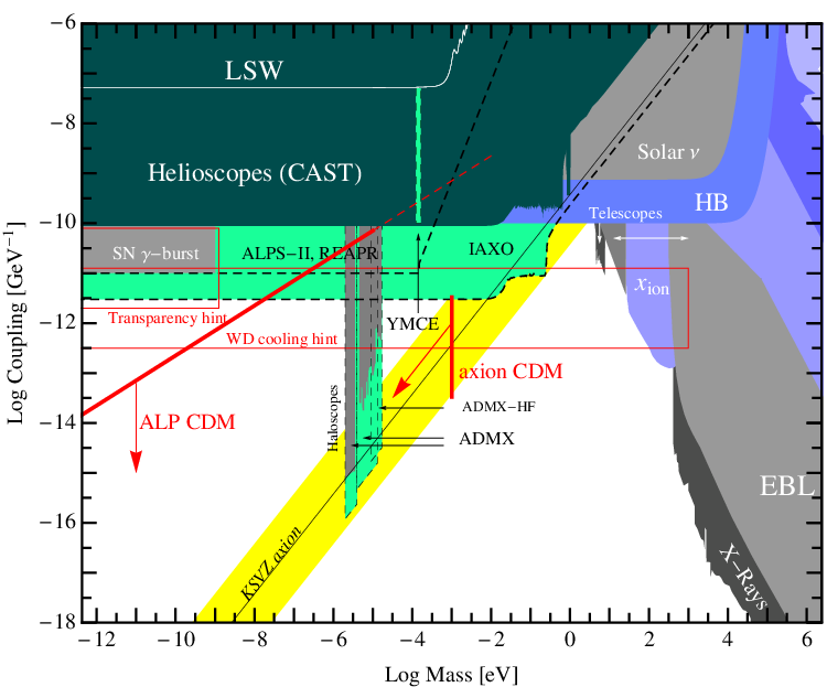
We have seen, that the LVS predicts – for the least fine-tuning of fluxes, such that $g_{s}\sim 0.1$ and $W_{0}\sim 1$, and a TeVish gravitino mass – an intermediate string scale and thus a QCD axion in the classic window, cf. Eq. (32). For decay constants in the upper part of this window, $f_{a}\gtrsim 10^{11\div 12}$ GeV, the QCD axion is expected to contribute substantially to the cold dark matter in the universe, see Eq. (6). Therefore, the intermediate string scale LVS can be probed by haloscope searches for axion cold dark matter [43] such as ADMX [44, 45, 46, 47]. These experiments exploit the coupling (4) by searching for the signal of dark matter axion to photon conversions in a narrow bandwidth microwave cavity sitting in a strong magnetic field. As can be seen from the light green area in Fig. 3 labelled as “Haloscopes”, a substantial range of the QCD axion dark matter parameter range will be probed by ADMX and other haloscopes [48] in the next decade.

A complementary search for the QCD axion in the lower part of the classic window, $f_{a}\gtrsim 10^{9\div 10}$ GeV, can be conducted with the next generation of axion helioscopes [43], in which one tries to detect solar axions by their conversion into photons inside of a strong magnet pointed towards the sun. Indeed, the projected sensitivity of the proposed International Axion Observatory IAXO [52] covers nicely a part of QCD axion parameter space which will not be covered by the haloscope searches, as can be seen in Fig. 3.

A very welcome feature of helioscopes is that they do not lose sensitivity towards low masses: their projected sensitivity are best and stay constant at small masses, see Fig. 3. That means, with IAXO one may also probe the LVS axiverse, in particular the possible existence of more ALPs with approximate the same coupling to photons as the QCD axion.

This is very important in view of recent tantalising astrophysical hints, such as the anomalous transparency of the Universe for TeV photons [53] and the anomalous cooling of white dwarfs [54, 55], which could be explained by the existence of an ALP with decay constants, couplings and mass [56, 57, 58, 59, 60, 61, 62]:

compatible with the prediction of an intermediate string scale LVS axiverse with $C_{i\,\gamma}/C_{i\,e}\sim 10$. The projected sensitivity of IAXO nicely overlaps with the ALP parameter region required to explain these hints, see Fig. 3.

Intriguingly, this parameter region for ALPs can also be partially probed by purely laboratory based light-shining-through-walls experiments [63], where laser photons are send along a strong magnetic field, allowing for their conversion into ALPs, which may then reconvert in the strong magnetic field behind a blocking wall into photons, apparently shining through the wall and susceptible to detection. The projected sensitivities of the proposed experiments ALPS-II at DESY and REAPR at Fermilab partially cover the expectations (34) from an intermediate string scale LVS axiverse and from the hints (38) from astrophysics, see Figs. 1 and 3.

References

- [1] Weinberg S 1978 Phys. Rev. Lett. 40 223
- [2] Wilczek F 1978 Phys. Rev. Lett. 40 279
- [3] Peccei R D and Quinn H R 1977 Phys. Rev. Lett. 38 1440
- [4] Georgi H, Kaplan D B and Randall L 1986 Phys. Lett. B 169 73
- [5] Kim J E 1979 Phys. Rev. Lett. 43 103
- [6] Dine M, Fischler W and Srednicki M 1981 Phys. Lett. B 104 199
- [7] Shifman M A , Vainshtein A I and Zakharov V I 1980 Nucl. Phys. B 166 493
- [8] Zhitnitsky A R 1980 Sov. J. Nucl. Phys. 31 260 [1980 Yad. Fiz. 31 497]
- [9] Bardeen W A and Tye S-H H 1978 Phys. Lett. B 74 229
- [10] Kaplan D B 1985 Nucl. Phys. B 260 215
- [11] Srednicki M 1985 Nucl. Phys. B 260 689
- [12] Preskill J, Wise M B and Wilczek F 1983 Phys. Lett. B 120 127
- [13] Abbott L F and Sikivie P 1983 Phys. Lett. B 120 133
- [14] Dine M and Fischler W 1983 Phys. Lett. B 120 137
- [15] Witten E 1984 Phys. Lett. B 149 351
- [16] Conlon J P 2006 JHEP 0605 078
- [17] Svrcek P and Witten E 2006 JHEP 0606 051
- [18] Conlon J P 2006 Phys. Rev. Lett. 97 261802
- [19] Choi K-S, Kim I-W and Kim J E 2007 JHEP 0703 116
- [20] Arvanitaki A et al, 2010 Phys. Rev. D 81 123530
- [21] Acharya B S, Bobkov K and Kumar P 2010 JHEP 1011 105
- [22] Cicoli M, Goodsell M and Ringwald A 2012 Preprint arXiv:1206.0819 [hep-th]
- [23] Grimm T W and Louis J 2004 Nucl. Phys. B 699 387
- [24] Jockers H and Louis J 2005 Nucl. Phys. B 705 167
- [25] Goodsell M, Jaeckel J, Redondo J and Ringwald A 2009 JHEP 0911 027
- [26] Cicoli M, Goodsell M, Jaeckel J and Ringwald A 2011 JHEP 1107 114
- [27] Banks T, Dine M and Gorbatov E 2004 JHEP 0408 058
- [28] Donoghue J F 2004 Phys. Rev. D 69 106012 [2004 Erratum-ibid. D 69 129901]
- [29] Gukov S, Vafa C and Witten E 2000 Nucl. Phys. B 584 69
- [30] Giddings S B, Kachru S and Polchinski J 2002 Phys. Rev. D 66 106006
- [31] Kachru S, Kallosh R, Linde A and Trivedi S P 2003 Phys. Rev. D 68 046005
- [32] Bobkov K, Braun V, Kumar P and Raby S 2010 JHEP 1012 056
- [33] Balasubramanian V, Berglund P, Conlon J P and Quevedo F 2005 JHEP 0503 007
- [34] Cicoli M, Mayrhofer C and Valandro R 2012 JHEP 1202 062
- [35] Cicoli M 2012 these proceedings
- [36] Conlon J P, Quevedo F and Suruliz K 2005 JHEP 0508 007
- [37] Becker K, Becker M, Haack M and Louis J 2002 JHEP 0206 060
- [38] Collinucci A et al 2009 JHEP 0907 074
- [39] Balasubramanian V and Berglund P 2004 JHEP 0411 085
- [40] Westphal A 2007 JHEP 0703 102
- [41] Rummel M and Westphal A 2012 JHEP 1201 020
- [42] Louis J, Rummel M, Valandro R and Westphal A Preprint arXiv:1208.3208 [hep-th]
- [43] Sikivie P 2983 Phys. Rev. Lett. 51 1415 [1984 Erratum-ibid. 52 695].
- [44] Asztalos S J et al 2001 Phys. Rev. D 64 092003
- [45] Asztalos S J et al [The ADMX Collaboration] 2010 Phys. Rev. Lett. 104 041301
- [46] Asztalos S J et al 2011 Nucl. Instrum. Meth. A 656 39
- [47] Heilman J et al [ADMX Collaboration] 2010 AIP Conf. Proc. 1274 115
- [48] Baker O K et al 2012 Phys. Rev. D 85 035018
- [49] Redondo J 2012 private communication
- [50] Arias P, Cadamuro D, Goodsell M, Jaeckel J, Redondo J and Ringwald A 2012 JCAP 1206 013
- [51] Hewett J L et al. 2012 Preprint arXiv:1205.2671 [hep-ex]
- [52] Irastorza I G et al 2011 JCAP 1106 013
- [53] Horns D and Meyer M 2012 JCAP 1202 033
- [54] Isern J, Garcia-Berro E, Torres S and Catalan S 2008 Astrophys. J. 682 L109
- [55] Isern J, Catalan S, Garcia-Berro E and Torres S 2009 J. Phys. Conf. Ser. 172 012005
- [56] De Angelis A, Mansutti O, Roncadelli M 2007 Phys. Rev. D76 121301
- [57] Simet M, Hooper D, Serpico P D 2008 Phys. Rev. D77 063001
- [58] Sanchez-Conde M A et al 2009 Phys. Rev. D79 123511
- [59] Dominguez A, Sanchez-Conde M A and Prada F 2011 JCAP 1111 020
- [60] Tavecchio F, Roncadelli M, Galanti G and Bonnoli G 2012 Preprint arXiv:1202.6529 [astro-ph.HE]
- [61] Isern J et al, 2012 Preprint arXiv:1204.3565 [astro-ph.SR]
- [62] Horns D et al 2012 Preprint arXiv:1207.0776 [astro-ph.HE]
- [63] Redondo J and Ringwald A 2011 Contemp. Phys. 52 211