Computational information geometry: theory and practice
Abstract
This paper lays the foundations for a unified framework for numerically and computationally applying methods drawn from a range of currently distinct geometrical approaches to statistical modelling. In so doing, it extends information geometry from a manifold based approach to one where the simplex is the fundamental geometrical object, thereby allowing applications to models which do not have a fixed dimension or support. Finally, it starts to build a computational framework which will act as a proxy for the Ôspace of all distributionsÕ that can be used, in particular, to investigate model selection and model uncertainty. A varied set of substantive running examples is used to illustrate theoretical and practical aspects of the discussion. Further developments are briefly indicated.
keywords
[class=AMS] Primary 62F99 ; secondary 62-04keywords
Information geometry , Multinomial distribution , Affine geometry , Exponential family , Extended exponential familyLondon School of Hygiene and Tropical Medicine, Keppel Street, London WC1E 7HT, UK ??
and
Department of Mathematics and Statistics, The Open University, Walton Hall, Milton Keynes, Buckinghamshire. MK7 6AA, UK
??
and
Department of Statistics and Actuarial Science, University of Waterloo, 200 University Avenue West, Waterloo, Ontario, Canada N2L 3G1
??
and
Department of Biostatistics, East Carolina University 2435C Health Sciences Building, Greenville, NC 27858-4353 USA
??
1 Introduction
The application of geometry to statistical theory and practice has produced a number of different approaches and this paper will involve three of these. The first is the application of differential geometry to statistics, which is often called information geometry. It largely focuses on typically multivariate, invariant and higher-order asymptotic results in full and curved exponential families through the use of differential geometry and tensor analysis; key references include [1], [6], [7], [30] and [21]. Also included in this approach are consideration of curvature, dimension reduction and information loss, see [13] and [27]. The second important, but completely separate, approach is in the inferentially demanding area of mixture modelling, a major highlight being found in [25] where convex geometry is shown to give great insight into the fundamental problems of inference in these models and to help in the design of corresponding algorithms. The third approach is the geometric study of graphical models, contingency tables, (hierarchical) log-linear models, and related topics involving the geometry of extended exponential families. Important results with close connections to the approach in this paper can be found in [34] and [14], while the wider field of algebraic statistics is well-reviewed in [32] and [16].
This paper has the following four objectives: (1) to use the tool of the extended multinomial distribution (see [8], [34], [14] and [11]) to construct a framework which unifies all of the above geometric approaches; in particular, to show explicitly the links between information geometry, extended exponential families and Lindsay’s mixture geometry, (2) to show how this unifying framework provides a natural home for numerically implementing algorithms based on the geometries described above, (3) to extend the results of information geometry from the traditional manifold based approach to models which do not have a fixed dimension or support, and (4) to start to build a computational framework which will act as a proxy for the ‘space of all distributions’ which can be used, in particular, to investigate model selection and model uncertainty. This paper lays the conceptual foundations for these goals, with more detailed developments to be found in later work. We call this numerical way of implementing geometric theory in statistics computational information geometry. No confusion should arise from the fact that the same name is given to a cognate, but distinct, topic in machine learning: see for example [31].
In practice, a single statistical problem can involve more than one of the above geometries – potentially all three – this plurality being handled naturally in our unifying framework. Indeed, we use a varied set of substantive running examples to illustrate theoretical and practical aspects of the development. Examples 1 and 4 (Section 1.1) are chosen to illustrate computational information geometric issues in mixture models. Example 2 shows issues in full and curved exponential families, while Example 3 looks at the geometry of logistic regression. To aid with visualisation additional low dimensional multinomial models are also introduced in the body of the paper.
The key idea of this paper is to represent statistical models – sample spaces, together with probability distributions on them – and associated inference problems, inside adequately large but finite dimensional spaces. In these embedding spaces the building blocks of the three geometries described above can be numerically computed explicitly and the results used for algorithm development. In §1.2 and §6 we reflect on the generality of working in this finite, discrete framework even with models for continuous random variables.
Accordingly, after a possible initial discretisation, the space of all distributions for the random variable of interest can be identified with the simplex,
| (1.1) |
together with a unique label for each vertex, representing the random variable. Modulo discretisation, this structure therefore acts as a universal model. Clearly, the multinomial family on categories can be identified with the relative interior of this space, , while the extended family allows the possibility of distributions with different support sets.
The starting point for much of statistical inference is a working model for observed data comprising a set of distributions on a sample space. A working model can be represented by a subset of and may be specified by an explicit parameterisation, such as Example 2, or as the solution of a set of equations, such as Example 4. Computational information geometry explicitly uses the information geometry of to numerically compute statistically important features of . These features include properties of the likelihood, which can be nontrivial in many of the examples considered here, the adequacy of first order asymptotic methods – notably, via higher order asymptotic expansions – curvature based dimension reduction and inference in mixture models.
1.1 Examples
For ease of reference the main examples considered in this paper are briefly described here, together with the main points which they illustrate.
Example 1.
Mixture of binomial distributions This example comes from [22] where the authors state that ‘simple one-parameter binomial and Poisson models generally provide poor fits to this type of binary data’, and therefore it is of interest to look in a ‘neighbourhood’ of these models. The extended multinomial space is a natural place to define such a ‘neighbourhood’ and a new computational algorithm defined in §5 is used for inference.
Example 2.
Censored exponential This example looks at a continuous response variable – a censored survival time. Section 1.2 considers applying the results of computational information geometry to models for continuous random variables while Theorems 4.1 and 4.2 show how this can be done with negligible loss for inference. In this case also results on curvature based dimension reduction are illustrated.
Example 3.
Logistic regression This is a full exponential family that lies in a very high dimensional simplex when considered as a model for the joint distribution of binary response variates. In this example, both the existence of the maximum likelihood estimate (see [34] and [14]) and higher order approximations to sampling distributions are considered.
Example 4.
Tripod model The tripod example is discussed in [35] and [36]. The directed graph is shown in Fig. 1, where there are binary variables , , on each of the terminal nodes these being assumed independent given the binary variable at the internal node . In the model, it is assumed is hidden (i.e. not observed) so the model is a mixture of members of an exponential family. Despite the model’s apparent simplicity, the mixture structure can generate multiple modes in the likelihood, illustrating difficult identification issues.

1.2 Discretisation
The approach taken in this paper is inherently discrete and finite. Sometimes, this is with no loss at all, the models used involve only such random variables. In general, suitable finite partitions of the sample space can be used, for which an appropriate theory is developed. While this is clearly not the most general case mathematically speaking (an equivalence relation being thereby induced), it does provide an excellent foundation on which to construct a computational theory. Furthermore, since real world measurements can only be made to a fixed precision all models can – arguably, should – be thought of as fundamentally categorical. The relevant question for a computational theory is then: what is the effect on the inferential objects of interest of a particular selection of such categories? This is looked at in Theorem 4.1 and 4.2.
Example 2 (continued).
Here the data taken from [17], while being treated as continuous, is only recorded at integer number of days. Thus as far as any statistical analysis that can be carried out is concerned there is literally zero loss in treating it as sparse categorical. For Figs. 9 and 10 a further level of coarseness was added by selecting bins of size days. As can be seen from the likelihood plot, Fig. 9, there is effectively no inferential loss in such a choice.
1.3 Structure of paper
The paper is structured as follows. Section 2 looks at the information geometry of . It shows the geometry to be both explicit and tractable. In particular, the way that global geometry determines the relationship between the natural and mean parameters of exponential families is discussed in §2.1. The Fisher information is also key and results on its spectrum are found in §2.2, while the shape of the likelihood function is discussed in §2.3. Section 3 looks at the importance of understanding the closure of , and of exponential families embedded in , where we consider the computation of limit points and the corresponding behaviour of maximum likelihood estimates. Direct applications of the numerical approach are discussed in Section 4. Issues considered include: using higher order asymptotic methods, such as Edgeworth and saddlepoint expansions and, also, dimension reduction and information loss. Section 5 looks at the way that the mixture geometry of [25] fits naturally into the computational information geometry framework. In this section, Examples 1 and 4 show the utility of the methods. Again the issue of dimension, this time in the -geometry, comes to the fore. Throughout, proofs and more technical discussions are found in the appendices.
2 Geometry of extended multinomial distribution
The key idea behind computational information geometry is that models can be embedded in a computationally tractable space with little loss to the inferential problem of interest. Information geometry is constructed from two different affine geometries related in a non-linear way via duality and the Fisher information, see [1] or [21]. In the full exponential family context, one affine structure (the so-called structure) is defined by the natural parameterization, the second (the structure) by the mean parameterization. The closure of exponential families has been studied by [4], [8], [23] and [33] in the finite dimensional case and by [11] in the infinite dimensional case. One important difference in the approach taken here is that limits of families of distributions, rather than pointwise limits, are central.
This paper constructs a theory of information geometry following that introduced by [1] via the affine space construction introduced by [30] and extended by [26]. Since this paper concentrates on categorical random variables, the following definitions are appropriate. Consider a finite set of disjoint categories or bins . Any distribution over this finite set of categories is defined by a set which defines the corresponding probabilities.
Definition 2.1.
The -affine space structure over distributions on is where
and the addition operator is the usual addition of sequences.
In Definition 2.1 the space of (discretised) distributions is a -convex subspace of the affine space . A similar affine structure for the -geometry, once the support has been fixed, can be derived from the definitions in [30].
The extended multinomial family, over -categories, characterized by the closed simplex of probabilities defined in (1.1) will be the computationally tractable space. For these families, the dual affine geometries are explicit, the only ‘hard’ computational tasks being the non-linear mapping between convex subsets of affine spaces and the computation of the mixed parameterization, as defined in [5]. Furthermore, the Fisher information and its inverse are explicit and, perhaps more relevantly due to its potentially high order (the dimension of the simplex) and non-constant rank, there are good ways of understanding and bounding its spectrum, as shown in §2.2.
It is important to clarify why the closed extended multinomial distribution is used. First, in many examples the data is sparse in the sense that the sample size is much smaller than , the number of categories, so that the likelihood, both in the multinomial and sometimes in the embedded models, is typically maximized on the boundary. Second, it will be shown that the global shape of the likelihood function is determined by boundary behaviour. Third, first order asymptotic approximations are rarely uniform across and the higher order asymptotic expansions of computational information geometry can indicate when the boundary is inferentially relevant. Finally, the link between information geometry and Lindsay’s mixture geometries is defined by using the boundary of .
The probability simplex, and sub-models embedded in it, have been extensively studied in the geometric approach to graphical models, see [34], [14]. In this literature, other sampling schemes than the multinomial are also studied, boundary issues again being shown to have great importance. One of the important new features here is the application of the full information geometry machinery to these models.
2.1 Geometry of extended trinomial distribution
To illustrate the information geometry of the extended multinomial distribution, the trinomial case is now described explicitly. The general case in fact will follow by obvious extensions, and shown later (Section 3.1), unless the dimension is so large that numerically evaluating sums becomes impractical, see [15].
Example 5.
An explicit example of the information geometry of the extended trinomial model is shown in Fig. 2. The closed simplex in panel (a) represents the set of multinomial distributions with bin probabilities where .
In this example, the vector was chosen, and the parallel lines in panel (a) are level sets of the mean of , where is the trinomial random variable. In the terminology of classical information geometry, these are -geodesics, and it is immediate that they extend to the boundary in a very natural way. These lines lie in the (tangent) direction which satisfies , and These lines are also shown in panel (b), but now in the (or natural) parameterization and so are non-linear. Note that the single line, labelled by the mean value equalling , corresponds to the geodesic passing through the vertex at in panel (a).
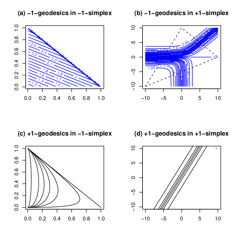
Panel (d) shows the relative interior of the extended trinomial in the natural affine parameterization. The straight lines represent one dimensional full exponential families with probabilities of the form
each . These are -geodesics in the direction through the base-point and, by the strict positivity of the exponential function, their image in panel (c) lie strictly in the interior of the simplex. It is a standard result that these parallel lines are everywhere orthogonal, with respect to the metric defined by the Fisher information matrix, to the -parallel lines shown in panels (a) and (b). Each of these parallel lines can be found by moving the base-point by
, where is restricted so that all components remain non-negative, [26].
The key step in understanding the simplicial nature of the -geometry is to see how the limits of the -parallel lines are connected to the boundary of the simplex. This is made clear in panel (c), where the -geodesics are plotted in the -affine parameters as curves. As changes the limits of the curves clearly exist and lie on the boundary of the simplex. The closure of the -representation multinomial is defined to make these continuous limits defined “at infinity” in the -parameters and is shown schematically as the dotted triangle in panel b.
2.2 Spectrum of Fisher Information
The material above looks explicitly at the -affine geometries of [1] while this section concentrates on the third part of Amari’s structure, i.e. the Fisher information or -geometry. In any multinomial model, the Fisher information matrix and its inverse are explicit. Indeed, the -geodesics and the corresponding geodesic distance are also explicit, see [1] or [21]. However, since the simplex glues together multinomial structures with different supports, and the computational theory is in high dimensions, it is a fact that the Fisher information matrix can be arbitrarily close to being singular. It is therefore of central interest that the spectral decomposition of the Fisher information itself has a very nice structure, as shown in this section.
Example 6.
Consider a multinomial distribution based on categories of equal width on , where the probability associated to a bin is proportional to that of the standard normal distribution for that bin. The Fisher information for this model is an matrix whose spectrum is shown in Fig. 3. By inspection it can be seen that there are exponentially small eigenvalues, so that while the matrix is positive definite it is also arbitrarily close to being singular. Furthermore, it can be seen that the spectrum has the shape of a half-normal density function and that the eigenvalues seem to come in pairs. These facts are direct consequences of the following results.

With denoting the vector of all bin probabilities except , the Fisher information matrix for the parameters, written as a function of the probabilities, is the sample size times
whose explicit spectral decomposition given, in all cases, in Appendix 1, is an example of interlacing eigenvalue results, (see for example [18], Chapter 4). In particular, suppose comprises distinct values , occuring times, so that . Then, the spectrum of comprises simple eigenvalues satisfying
| (2.1) |
together, if , with , each such having multiplicity . Further, while each is typically (much) closer to than to , making it a near replicate of .
In this way, the Fisher spectrum mimics key features of the bin probabilities. Of central importance, one or more eigenvalues are exponentially small if and only if the same is true of the bin probabilities, the Fisher information matrix being singular if and only if one or more of the vanishes. Again, typically, two or more eigenvalues will be close when two or more corresponding bin probabilities are. We see this in Example 6 where, by symmetry of the distribution, the bin probabilities are paired, so that . The (decreasingly) ordered plot of the eigenvalues, Figure 3, then resembles two copies of the half-density formed by folding at the mode. These dominant features are robust to which bin we omit in forming and to asymmetric placing of the bins.
2.3 Likelihood in the simplex
Potentially high dimensional simplicial structures being the natural spaces in which to base computational information geometry, a primary question is to look at the way that the likelihood, or log-likelihood, behaves in them. First note two important issues: in typical applications the sample size will be much smaller than the dimension of the simplex, while the simplex contains sub-simplexes with varying support. These two statements mean that our standard intuition about the shape of the log-likelihood function will not hold. In particular, the standard -approximation to the distribution of the deviance does not hold.
It will be convenient to call the face of the simplex spanned by the vertices (bins) having strictly positive counts the observed face, and the face spanned by the complement of this set the unobserved face. In the -representation, the log-likelihood is strictly concave on the observed face, strictly decreasing in the normal direction from it to the unobserved face and, otherwise, constant. This is illustrated – a schematic representation of the quadrinomial case when there are two zeros in the vector of counts – in Figure 4, the -flat subspaces being formalised in Theorem 2.1.

The following theorem characterises the shape of the log-likelihood function in the -representation on the simplex. This function is concave, but not strictly concave, so, the theorem characterises where the lack of strict concavity comes from. Being given by the function , with the constraints and it is immediate that the log-likelihood is constant on subsets defined by fixing and varying . The decomposition presented in part (b) of the theorem shows that these subsets are, in fact, contained in -1-affine subspaces.
Theorem 2.1.
Let the observed counts be and define two subsets of the index set by and . Let , and further define the set by .
(a) The set is a linear subspace of . The log-likelihood is constant on affine subspaces of the form
(b) Select and consider the vector subspace of defined by
Then can be decomposed as a direct sum of vector spaces .
Proof.
See Appendix. ∎
3 Closure of exponential families
This section shows how the closure of exponential families plays a role in the computational geometry. In §3.1 the discussion of §2.1 is formalised and connected to the information geometric concept of duality. Furthermore, in §3.2 Example 3 is used to illustrate the fact that the way that the boundaries of the high dimensional simplex are attached to the model is of great importance for the behaviour of the likelihood and the for distribution of important inferential statistics.
3.1 Duality
One of the key aspects of information geometry is the relationship between the , and Fisher metric or -geometric structures via the concept called duality. Following [1] when the underlying geometric object is a manifold the relationship between the and connections, denoted by and and the Fisher information is captured in the duality relationship which can be written in terms of the inner product at , , and any vector fields via the equation
| (3.1) |
One consequence of this relationship is the existence on exponential families of a so-called mixed parameterization of the form , where is -affine and is -affine, their level sets being Fisher orthogonal across the manifold: see [5].
The following definition gives a useful computational tool for understanding the limiting behaviour of exponential subfamilies in , and gives a generalisation of the trinomial model shown in Fig. 2.
Definition 3.1.
Let be a probability vector, be a set of vectors in , such that
are linearly independent, and be a set of linearly independent vectors in such that for and . Furthermore, define
in which , and
| (3.2) |
where
| (3.3) |
Note that for fixed the image of is a -dimensional exponential family. As changes these exponential families are -parallel. However for fixed , the image of is not in general -affine, but is for the special case when . Thus this construction, while having the advantage of being explicit, is not as strong as a true mixed parameterisation. However, the function defined in Definition 3.2 is a useful tool in understanding the limiting properties of exponential families within the extended multinomial model. Consider the set of possible values of . By condition (3.3) it follows that the domain of – for given – is a polytope. As converges to the boundary of this polytope the corresponding exponential family converges to an extended exponential family defined on the boundary of determined by the corresponding zeros in the probability vector. This construction generalises the plots in Fig. 2 (c) and (d). Notice also that it allows the definition of the limits of families which complements the pointwise limits defined in [8] and [11].
3.2 Computing limits in exponential families

Example 7.
In order to visualise the geometric s of the problem of computing limits in exponential families consider a low dimensional example. Define a two dimensional full exponential family by the vectors and the uniform distribution base point, embedded in the three dimensional simplex. The -dimensional family is defined by the -affine space through spanned by the space of vectors of the form
Consider directions from the origin found by writing giving, for each , a one dimensional full exponential family parameterized by in the direction . The aspect of this vector which determines the connection to the boundary is the rank structure of its elements. For example, suppose the first component was the maximum and the last the minimum, then as this one dimensional family will be connected to the first and fourth vertex of the embedding four simplex, respectively. Note that changing the value of changes the rank structure, as illustrated in Fig. 5. In this plot, the four linear functions of are plotted (dashed lines) and the the impact of rank structure is determined by the upper and lower envelopes (solid lines). From this analysis of the envelopes of a set of linear functions it can be seen that the function is redundant. The consequence of this is shown in Fig. 6 which shows the result of direct computation in the two dimensional family. It is clear that, indeed, only three of the four vertexes of the ambient 4-simplex have been connected by the model.
In general, the problem of finding the limit points in full exponential families inside simplex models is a problem of finding redundant linear constraints. As shown in [12], this can be converted, via duality, into the problem of finding extremal points in a finite dimensional affine space.

Example 3 (continued).
Consider an design matrix with samples and a binary response . Let so that , the logistic regression model being given by
where is the row of . This is a full exponential family that lies in the simplex when considered a model for the joint distribution of the binary response variates. A design matrix defines a -dimensional -affine subset and changing the explanatory variates changes the direction of this low dimensional space inside the space of joint distributions.
Consider response data (0, 1, 0, 1, 0, 1, 1), the explanatory variables being and . For convenience, in the space of all joint distributions, label the bin associated with the sequence with the binary number which that sequence represents
| (3.4) |
This logistic model is a two-dimensional exponential family which passes through the point corresponding to the uniform distribution of the simplex and lies in the directions defined by
where is the binary representation of vertex .

As in Example 7 consider the way that this two-dimensional exponential family is attached to the boundary using the envelope method. There are possible lines to consider and these are shown in Fig. 7. These lines whose duals are extremal points are plotted in red and it can clearly be seen that the upper and lower envelopes have been found. The corresponding vertices which the full exponential family reaches are given by vectors of the form with the structure either and for or and for .
We can see how this global geometry affects the inference. One immediate issue is that if the observed data is a sequence which is one of the vertices listed above then the corresponding MLE will also lie on the boundary. Thus, for example, if the observed data is there is a ‘regular’ turning point in -space. However if, instead, the data is the MLE does indeed go to infinity and has its maximum at the correct vertex. This result for in fact generalizes, when the explanatory variable is linear, to any . The corresponding vertices which the full exponential family reaches are again given by vectors of the form with one of the two structures identified above.
4 The tools of information geometry
In general, working in a simplex, boundary effects mean that standard first order asymptotic results can fail. Most standard methods are not uniform across the simplex. Therefore one way that the higher order asymptotic methods of information geometry have value is that they can be used to validate the region of parameter space where the first order method will be accurate. Example 2 has a continuous random variable with compact support and it is used to show how discretisation can be used to apply computational information geometry to such models.
4.1 Higher order asymptotics: Edgeworth expansions
One very powerful set of results from classical information geometry derives from the fact that geometrically based tensor analysis is well-suited for use in multi-dimensional higher order asymptotic analysis, see [6] or [29]. However, using this tensorial formulation is not without difficulty for the mainstream statistician. Its very efficient, tight notation may perhaps obscure rather than enlighten, while the resulting formulae can typically have a very large number of terms, making them rather cumbersome to work with explicitly. These obstacles to implementation are overcome by the computational approach described in this paper. The clarity of the tensorial approach is ideal for coding, while large numbers of additive terms, of course, are easy to deal with. Two more fundamental issues, which the global geometric approach of this paper highlight, concern numerical stability. The ability to invert the Fisher information matrix is vital in most tensorial formulae and so understanding its spectrum, as discussed in Section 2.2, is vital. Secondly numerical under and overflow near boundaries requires careful analysis and so understanding the way that models are attached to the boundaries of the extended multinomial models is equally important.
An important aspect of higher order methods is not just their accuracy in a given example, but the way that they can be used to validate first order methods. In cases like logistic regression first order methods are typically used for inference despite the fact that they are not uniformly accurate across the parameter space of interest. In the example below the fact that the Edgeworth expansion is far from normal acts as a diagnostic for the first order methods.
Example 3 (continued).
Consider Fig. 8 where the parameters of a two dimensional logistic family are such that the sampling distribution of the sufficient statistics is considerably far from normal. This is shown by the simulated sample of black points, the red contours, computed numerically from the Edgeworth expansion, showing a good fit with the simulation, but a distribution which is far from the first order approximation. As holds widely, in this example, the Edgeworth expansion is easy to compute numerically.

4.2 Continuity and compactness
In order to use the high dimensional simplex models with continuous random variables it is necessary to truncate and discretise the sample space into a finite number of bins. The following theorems show that the information loss in doing this is arbitrarily small for a fine enough discretisation and that the key to understanding the information in general is controlling the conditional moments in each bin of the random variables of interest, uniformly in the parameters of the model.
Theorem 4.1.
Let , , be a parametric family of density functions with common support each being continuously differentiable on the relative interior of , assumed non-empty. Further, let be compact,while
is uniformly bounded in by , say.
Then for any and for any sample size , there exists a finite, measurable partition of such that: for all , and for all
| (4.1) |
where and are the likelihood functions from the discretised and continuous distributions respectively.
Proof.
See Appendix. ∎
The following result looks at the case where the family that is discretised is itself an exponential family and so the tools of classical information geometry can be applied. In general, after discretisation a full exponential family does not remain full exponential and there is information loss. However, the following results show that this loss can be made small enough to be unimportant for inference and that all information geometric results on the two families can be made arbitrarily close.
Theorem 4.2.
Let , , be an exponential family which satisfies the regularity conditions of [1], p. 16. Further, assume that is uniformly continuous and is compact.
Then, for any , there exists a finite measurable partition of such that, for all choices of bin labels , all terms of Amari’s information geometry for can be approximated to by the corresponding terms for the family
In particular:
- (a)
For all , and any norm,
where and .
- (b)
The expected Fisher information for of , , and the expected Fisher information for , , satisfies
- (c)
The skewness tensors , see [1], p. 105, of and for satisfy
Proof.
See Appendix. ∎
The following Corollary states that the likelihood before and after discretisation can also be made arbitrarily close with a fine enough discretisation, as illustrated in Fig. 9 drawn from Example 2, as described below.
Corollary 4.1.
Under the conditions of Theorem 4.2, let denote the MLE based on a sample, , from and the MLE for based on the counts , for the partition of Theorem 4.2.
Then
| (4.2) |
and
| (4.3) |
Proof.
See Appendix.∎
The following example illustrates these results and also shows an application of dimension reduction based on information geometry. Dimension reduction is dependent on the choice of affine structure. The reduction here is done in the -affine geometry, unlike the mixture geometry examples, 1 and 4, where it is done in the -geometry.
Example 2 (continued).
This example shows how results from information geometry can be numerically implemented in the resultant curved exponential family. An example in [17] concerns survival times for leukaemia patients measured in days from the time of diagnosis. Originally from [9], there are 43 observations. For illustrative purposes the data is censored at a fixed value such that the censored exponential distribution gives a reasonable, but not perfect, fit. It is assumed the random variable has an exponential distribution but only is observed. As discussed in [28] this gives a one-dimensional curved exponential family inside a two dimensional regular exponential family of the form
| (4.4) |
where and and the embedding map is given by .


Figure 9 shows some of the details of the geometry of the curved exponential family which is created after censoring. The censoring value was chosen at 750. The parameter of interest is , the mean of the uncensored observations. In the left hand panel of Fig. 9, the solid line is the likelihood function based on binning the data to bins of width four days and using a multinomial approximation. The dots in this panel are the log-likelihood for the raw data based on the continuous censored exponential model. As can be clearly seen there is no real inferential loss in the binning and discretisation process. The likelihood plot also shows appreciable skewness, which suggests that standard first order asymptotics might be improved by the higher order asymptotic methods of classical information geometry.
The right hand panel shows the censored exponential (solid curve) embedded in the two-dimensional full exponential family in the -parameterization. The dashed contours are the log-likelihood contours in the full exponential family. It is clear, even visually, that there is not much curvature for this family on this inferential scale. So this is an example where the curved exponential family behaves inferentially like a one-dimensional full exponential family. In particular, the dimension reduction techniques found in [27], can be used. To see the effectiveness of this idea, Fig. 10 shows how well a saddlepoint based approximation does at approximating the distribution of the maximum likelihood estimator of the parameter of interest.
4.3 Higher order asymptotics: saddlepoint method
The saddlepoint approximation method is very important tool from classical information geometry, see Fig. 10 for an example. Using this method requires the solving of the so-called saddlepoint equation in an efficient and accurate manner and so for computational information geometry this only needs to be done numerically. The problem of solving this non-linear equation is tied to understanding the non-linear relationship between the and -parameters, and hence the rigorous implementation of numerical methods requires understanding the global geometry described above. For example, the issues surrounding such implementation being far from uniform across the simplex, it will help to be made aware if the method is being attempted in a region where first order asymptotics would work well or not.
Example 2 (continued).
Example 2 is a curved exponential family, [21]. Consider Fig. 11, this shows the level sets of the mean parameterization for the -dimensional family plotted in the natural parameters. Solving the saddlepoint equation requires mapping between these two coordinate systems. The figure illustrates the issues which need considering in implementing numerical methods to do this. At point ‘A’ in the figure we see that the level sets of the mean parameter are becoming close to parallel – this reflects the fact that the Fisher information can be very close to singular, as discussed in §2.2. At the point ‘B’ the bifurcation in the parameters, described in §2.1, is clear. Again, the point ‘C’ shows a region where there is close to linearity between the two coordinate systems which is typical of when first order asymptotic methods work well, see §4.1.

5 Inference on Mixtures
5.1 Lindsay’s geometry and the simplex
This section describes the way the mixture geometry of [25] is related to the information geometry of the simplex. In particular, it will lead to extending Lindsay’s structure in a way which will give considerable computational advantages in, for example, computing the non-parametric maximum likelihood estimate of a mixture model and understanding its variability.

Lindsay’s geometry lies in an affine space which is determined by the observed data. In particular, it is always finite dimensional, and the dimension is determined by the number of distinct observations. Following the notation of [24], which looks at mixtures of the model i.e. models of the form , let represent the distinct likelihood values of arising from the data . The likelihood on the space of mixtures is defined on the convex hull of the image of the map
Then the problem of finding the non-parametric likelihood estimate, determined by , is found by maximising a concave function over this convex set.
There are clear parallels between the convex geometry of Lindsay and the embedding in the -simplex. Lindsay’s geometry is designed for working with the likelihood so only concerns the observed data, rather than the full sample space. For simplicity consider discrete models where the distinct likelihood components are represented by probabilities where, by definition, lies in the observed face defined in Theorem 2.1 (Section 2.3). The affine structure of Lindsay is thus determined by the vertices of , see Fig. 12.
Definition 5.1.
Define to be the Euclidean orthogonal projection from a simplex to the smallest vector space containing the vertices indexed by .
The following result is strongly connected to Theorem 2.1. In it, the level sets of the likelihood are now characterised as the pre-images of the mapping . It also shows that searching for the maximum likelihood in the convex hull in the simplex is the same as in Lindsay’s geometry.
Theorem 5.1.
a) The likelihood on the simplex is completely determined by the likelihood on the image of . In particular, all elements of the pre-image of have the same likelihood value.
(b) maps convex hulls in the -simplex to the convex hull of Lindsay’s geometry.
Proof.
See Appendix. ∎
Given this result, it is natural to study the likelihood of a convex hull in the simplex rather than in Lindsay’s space. There are some definite advantages to this, some of which will be explored in this paper, while others will only be briefly mentioned. In Sections 5.2 and 5.3 a new search algorithm is proposed which exploits the information geometry of the simplex. In particular, it exploits dimension reduction directly in the simplex to give a direct way of computing the non-parametric maximum likelihood estimate.
A further advantage of working in the simplex is that while Theorem 5.1 shows that Lindsay’s geometry captures the and likelihood structure, it does not capture the full information geometry. For example, the expected Fisher information cannot be represented, since it is a defined using the full sample space, and hence analysis of the variability of the non-parametric maximum likelihood estimate is more natural in the full simplex, rather than in the data-dependent space proposed by Lindsay.
5.2 Total positivity and local mixing
In order to consider dimension reduction in the simplex, and the corresponding dimension of the convex hull, this paper concentrates on the case where the mixture is over an exponential family. At first sight, Theorem 5.2 and the following comments may appear contradictory. First Theorem 5.2 shows that -convex hulls of full exponential families have maximal dimension in the simplex, whereas the concept of local mixing, and its extension to polytope approximation in Theorem 5.3, shows that there exist very good low dimensional approximations to these convex hulls. It is the existence of these low dimensional approximations which is exploited by the proposed algorithm. Using results on total positivity, we have
Theorem 5.2.
The -convex hull of an open subset of a generic one dimensional exponential family is of full dimension.
Proof.
See Appendix. ∎
In this result “generic” means that the tangent vector which defines the exponential family has components which are all distinct.
Theorem 5.2 can be contrasted with the results of [26] or [2] which state, under regularity and for many applications, mixtures of exponential families have accurate low dimensional representations. The essential resolution of this apparent contradiction is that if the segment of the curve for lies ‘close’ to a low dimensional -affine subspace, then all mixtures over also lie ‘close’ to this space. The following discussion is then concerned with the appropriate definition of ‘close’ for modelling purposes.
Motivated by the idea of a local mixture, consider how well a full exponential family can be approximated by a polygonal path which vertices , . Any point on this polygonal path will have the form
| (5.1) |
with . Define the segment . So, on top of the usual label switching identification issue with mixtures, there is additionally the identification problem induced by
| (5.2) |
when . While lack of identification is usually considered a statistical problem, computationally it restricts the space the likelihood needs to be optimised over. It will be shown that restricting attention to this space has considerable computational advantages.
Consider, then, the following definition and lemma.
Definition 5.2.
Given a norm , the curve and the polygonal path define the distance function by
Lemma 5.1.
If for all then any point in the convex hull of lies within of the convex hull of the finite set .
Proof.
By the triangle inequality. ∎
Let be the non-parametric maximum likelihood estimate for mixtures of the curve . A consequence of Lemma 5.1 is that, under the uniform approximation assumption, lies within of the convex hull of the polygon. The question is then what norm is appropriate for measuring the quality of the polygonal approximation.
Definition 5.3.
Define the inner product
for and such that for all . This defines a preferred point metric as discussed in [10]. Further, let be the corresponding norm.
As motivation for using such a metric, consider the Taylor expansion for the likelihood around when the maximum is defined by turning point conditions, i.e. occurs at a point in the interior of the simplex. Under these conditions, to high order, it follows that
| (5.3) |
So small dispersions, as measured by , correspond to small changes in likelihood values. Note that this is clearly not true under the standard Euclidean norm, where unbounded changes in likelihood values are possible.
Following [25], the maximum of the likelihood in a convex hull is determined by the non-positivity of directional derivatives, rather than turning points. So the following likelihood approximation theorem is appropriate.
Theorem 5.3.
Let be an exponential family, and a finite and fixed set of support points such that for all . Further, denote by and the maximum likelihood estimates in the convex hulls of and respectively, and by the global maximiser in the simplex. Then,
| (5.4) |
Proof.
See Appendix. ∎
5.3 Implementation of Algorithm
Algorithms using the polygonal approximation technique will be evaluated in detail in future work. Here a general outline is given and a couple of examples examined (Examples 1 and 4). The fundamental idea is to compute the convex hull of a finite number of points on the curve as an approximation to the convex hull of the curve itself. The positioning of the points can be decided by using singular value decomposition methods to see if the line segment joining consecutive points has small enough curvature. From these it is necessary to compute which bounds the uniform approximation of the curve by the polygon and then apply Theorem 5.3.
The first example implements the theorem for a mixture of binomials.
Example 1 (continued).
Consider the data discussed in [22] shown in part in Table 1. Mixture models are of interest scientifically since the data concerns frequency of implanted foetuses in laboratory animals, and it could be expected that there is underlying clustering. Simple plots shows over-dispersion relative to the variance of a fitted binomial model, which implies that a mixture approach might be appropriate.
| Number of dead implants | 0 | 1 | 2 | 3 | 4 | 5 | 6 | 7 |
| Frequency | 214 | 154 | 83 | 34 | 25 | 9 | 5 | 0 |
Using the polygonal approximation approach allows us to compute easily a good approximation to the mixture. The result can be shown in Fig. 13. The crosses show the fitted model with circles the data, here with a mixture over . We also see the mixing proportions and the directional derivative.

Note in this example the near perfect fit of the data with the mixture model. In terms of the simplex this is easily explained since the maximum likelihood estimate in the simplex, in this case, lies inside the convex hull of the binomial model.
Example 4 (continued).
For this example, the distribution of the random variables at all the observed nodes lies in the dimensional simplex, parameterized by the joint probabilities for . If were observed each node would be independent, so that conditionally on this space is -dimensional, and can be parameterized by the marginal probabilities. It is easy to show that the conditional model includes all vertices of the simplex, intersects six pairs of opposite edges and three pairs of opposite 2-faces. The full tripod model is a two component mixture over the three-dimensional full exponential family. Unlike the full convex hull of Example 1, the two component mixture model need not be convex in the -affine space and so can have a complex multimodal likelihood structure. In order to aid visualisation, we also consider here the corresponding bipod model, see Fig. 14

In the tri- and bi-pod examples, the unmixed model can be approximated with unions of -affine polytopes. These can then be used to compute likelihood objects on the two hull and convex hull very efficiently just using convex programming. On each polytope the likelihood has a unique maximum which may, or may not, be on its boundary. To see the whole two-hull structure, you just need to glue together this finite number of polytopes and their maxima. Local maxima in the likelihood correspond to internal maxima in the polytopes.
To see how to construct these approximating polytopes, consider Figure 14. The curved surface shown is a, so-called, ruled-surface intersecting the boundary in two pairs of opposite edges. Choose a finite number of support points on each edge of the surface and the same number on the opposed edge. Joining corresponding pairs of points gives a set of convex sets, or slices, close to the surface. Any point in the two hull – that is a convex combination of two points – lies in the convex polytope which is the convex hull of two of these slices.
6 Discussion and further work
This paper focused on four main objectives: (1) it showed that extended multinomial distributions can be used to construct a computational framework demonstrating commonality between the distinct areas of information geometry, mixture geometry and the geometry of graphical models, (2) it showed how this structure allow numerically implementation of results from these areas, (3) it extended results of information geometry to a simplicial based geometry for models which do not have a fixed dimension or support, and finally (4) it began the process of building a computational framework which will act as a proxy for the ‘space of all distributions’.
In continuous examples, a compactness condition is used to keep the underlying geometry finite. A following paper will look at the case where the compactness condition is not needed. In this case, infinite dimensional simplexes, and their closures, are used as the ‘space of all distributions’, the extension of classical information geometry here requiring careful consideration of convergence, not required here due to finiteness.
Later work will discuss a variety of statistical inference problems – including model selection and model uncertainty – using both these finite and infinite frameworks.
Acknowledgement
The authors gratefully thank EPSRC for the support of Grant Number EP/E017878/.
Appendix 1: On the spectral decomposition of the Fisher information
For notational convenience denote so that (i.e. bin is omitted in the vector ) and . Without loss, after permutation, assume . Apart from the trivial case , when vanishes, its spectral decomposition (SpD) comes in the following cases.
- Case 1
for some . The SpD of
where and , follows from that of given below.
- Case 2
is trivial.
- Case 3
. The SpD of is
where and . Here has multiplicity and eigen-space , while has multiplicity and eigen-space. In particular, using ,
- Case 4
This is the generic case. Denoting by the zero matrix of order , and by the rank one orthogonal projector onto Span(), , if , and , then the SpD is
where , and the are the zeros of
In particular, are simple eigenvalues satisfying (2.1) while, whenever , is also an eigenvalue having multiplicity . Further, expanding , we again find:
so that , as claimed. Finally, we note that each is typically (much) closer to than to . For, considering the graph of , is well-approximated by
whose unique zero over is positive whenever, as will typically be the case, (both will usually be ) while . Indeed, a straightforward analysis shows that, for any and , as .
Appendix 2: Proofs
Proof of Theorem 2.1.
(a) Immediate.
(b) Let so that and write as where
and
Then, it is immediate that is in and is in , the decomposition being clearly unique. ∎
Proof of Theorem 4.1.
Let be any finite measurable partition of . Then defining gives for and
where is a convex combination of and , [3] p. 124, Thm 6–22, and . Thus,
| (.1) | |||||
where and .
It is clear that for compact there exists a sequence of finite measurable partitions such that as
| (.2) |
From (.1) it follows that
so that
Since is bounded away from zero for all , this gives
from which the result follows.
∎
Proof of Theorem 4.2 .
Proof of Corollary 4.1.
The score equations for are , while from (.7) those for are
Using (.5) and that has a continuous inverse gives (4.2), while (4.3) follows from (4.2) and (.8).
∎
Proof of Theorem 5.1.
(a) The log-likelihood can be written as which is clearly constant for all probability vectors with the same image under since they share the same elements . (b) Since is linear it preserves convexity. ∎
Proof of Theorem 5.2.
For any with each , and , let have general element
Further, let , whose general column is . Then, it suffices to show that has rank . But, using [19] p.33, , so that
where . It suffices, then, to recall [20] that is strictly total positivity (of order ), so that .
∎
Proof of Theorem 5.3.
We use a similar expansion to (5.3), adapted to take into account the fact that the NPMLE is defined by directional derivatives being non-negative, rather than zero [25].
If is a member of the convex hull of then the directional derivative from to is a finite convex combination of elements of the convex cone of directional derivatives from to points in the curve . For any point consider the perturbation from of the form
There are two cases to consider: (i) either is a support point of or (ii) it is not.
Case (i) In this case the directional derivative are zero. Accordingly we can apply (5.3) directly to have that the change in log-likelihood is .
Case (ii) In this case, for small enough positive , remains in the convex hull. Further, the difference in log-likelihood values is then
Since the directional derivatives are now non-zero, consider the first order term in the Taylor expansion of this difference:
Considering small enough that
we have that to first order the change in log-likelihood values for points within of is bounded by
So it has been shown that all points in the convex hull of which are within of satisfy (5.4). From Lemma 5.1 there is at least one point in the convex hull of the polygon which is within of the convex hull. Hence the maximum likelihood value at also satisfies (5.4). ∎
References
- [1] S.-I. Amari. Differential-geometrical methods in statistics. Springer-Verlag, 1990.
- [2] K. Anaya-Izquierdo and P. Marriott. Local mixtures models of exponential families. Bernoulli, 13(3):623–640, 2007.
- [3] T.M. Apostol. Mathematical Analysis. Addison-Wesley:Reading, MA, 1965.
- [4] O.E. Barndorff-Nielsen. Information and exponential families in statistical theory. John Wiley & Sons, 1978.
- [5] O.E. Barndorff-Nielsen and P. Blaesild. Exponential models with affine dual foliations. Annals of Statist., 11(3):753–769, 1983.
- [6] O.E. Barndorff-Nielsen and D.R. Cox. Asymptotic techniques for use in statistics. Chapman & Hall, 1989.
- [7] O.E. Barndorff-Nielsen and D.R. Cox. Inference and asymptotics. Chapman & Hall, 1994.
- [8] L.D. Brown. Fundamentals of statistical exponential families: with applications in statistical decision theory. Institute of Mathematical Statistics, 1986.
- [9] M.C. Bryson and M.M. Siddiqui. Survival times: some criteria for aging. JASA, 64:1472–1483, 1969.
- [10] F. Critchley, P. Marriott, and M. Salmon. Preferred point geometry and statistical manifolds. The Annals of Statistics, 21:1197–1224, 1993.
- [11] I. Csiszar and F. Matus. Closures of exponential families. The Annals of Probability, 33(2):582–600, 2005.
- [12] H. Edelsbrunner. Algorithms in combinatorial geometry. Springer-Verlag: NewYork, 1987.
- [13] B. Efron. Defining the curvature of a statistical problem (with applications to second order efficiency). The Annals of Statistics, 3(6):1189–1242, 1975.
- [14] S Feinberg and A. Rinaldo. Maximum likelihood estimation in log-linear models: Theory and algorithms. arxiv:1104.3618v1, 2011.
- [15] D. Geiger, D. Heckerman, H. King, and C. Meek. Stratified exponential families: Graphical models and model selection. Annals of Statistics, 29(2):505–529, 2001.
- [16] P. Gibilisco, E. Riccomagno, M.P. Rogantin, and H.P. Wynn. Algebraic and Geometric Methods in Statistics. New York, NY: Cambridge University Press, 2010.
- [17] D.J. Hand, F. Daly, A.D. Lunn, K.J. McConway, and E. Ostrowski. A handbook of small data sets. Chapman and Hall, London, 1994.
- [18] R.A. Horn and C.R. Johnson. Matrix Analysis. CUP, 1985.
- [19] A.S. Householder. The Theory of Matrices in Numerical Analysis. Dover Publications, 1975.
- [20] S. Karlin. Total Positivity, Vol. I. Stanford University Press, 1968.
- [21] R.E. Kass and P.W. Vos. Geometrical foundations of asymptotic inference. John Wiley & Sons, 1997.
- [22] L.L. Kupper and J.K. Haseman. The use of a correlated binomial model for the analysis of certain toxicological experiments. Biometrics, 34(1):69–76, 1978.
- [23] S.L. Lauritzen. Graphical models. Oxford University Press, 1996.
- [24] M.L. Lesperance and J.D. Kalbfleisch. An algorithm for computing the nonparametric MLE of a mixing distribution. Journal of the American Statistical Association, 87:120–126, 1992.
- [25] B.G. Lindsay. Mixture Models: Theory, Geometry, and Applications. Institute of Mathematical Statistics, 1995.
- [26] P. Marriott. On the local geometry of mixture models. Biometrika, 89(1):77–93, 2002.
- [27] P. Marriott and P.W. Vos. On the global geometry of parametric models and information recovery. Bernoulli, 10:639–649, 2004.
- [28] P. Marriott and S. West. On the geometry of censored models. Calcutta Statistical Association Bulletin, 52:235–249, 2002.
- [29] P. McCullagh. Tensor methods in statistics. Chapman & Hall, 1987.
- [30] M.K. Murray and J.W. Rice. Differential geometry and statistics. Chapman & Hall, 1993.
- [31] F. Nielsen. Computational information geometry: Pursuing the meaning of distances. In Open Systems Science. 2009. (in Japanese).
- [32] G. Pistone, E. Riccomagno, and H.P. Wynn. Algebraic Statistics: Computational Commutative Algebra in Statistics. Chapman and Hall, 2000.
- [33] A. Rinaldo. On maximum likelihood estimation in log-linear models. Tech. Rep. Dep. of Statistics, Carnegie Mellon University, 2006.
- [34] A. Rinaldo, Feinberg S., and Zhou Y. On the geometry of discrete exponential families with applications to exponential random graph models. Electron. J. Statist., 3:446–484, 2009.
- [35] P. Zwiernik and J.Q. Smith. Implicit inequality constraints in a binary tree model. Electron. J. Statist., 5:1276–1312, 2011.
- [36] P. Zwiernik and J.Q. Smith. Tree-cumulants and the geometry of binary tree models. Bernoulli, 18(1):290–321, 2012.