Density of states and extent of wave function:
two crucial factors for small polaron hopping conductivity in 1D

In the context of GMCM we consider a 1D deformable “wire” consisting of “molecular lattice sites” across which small polarons are transported in the presence of disorder. By $\epsilon_{i}(0)$, and $\epsilon_{j}(0)$ we denote the energies of an electron on site at vector positions $\mathbf{r}_{i}$ and $\mathbf{r}_{j}$, respectively, if the “molecular lattice sites” are constrained not to be displaced in response to the presence of the electron. Due to the disorder these local electronic energies, $\epsilon_{i}(0)$, and $\epsilon_{j}(0)$ are not equal. The energetic non-equivalence of the two sites will affect the small polaron’s binding energy, $E_{b}(i)$, in the sense that, the lower the local electronic energy is the more localized the electronic wave function will tend to be and consequently the larger its binding energy will be. Assuming that the stiffness of the “molecular lattice” is unaltered, the difference in binding energy means a difference in the electron-lattice interaction parameters $A_{i}$ and $A_{j}$ i.e. $E_{i}(\mathbf{x}_{i})=\epsilon_{i}(0)-A_{i}\mathbf{x}_{i}$ and $E_{j}(\mathbf{x}_{j})=\epsilon_{j}(0)-A_{j}\mathbf{x}_{j}$ with $A_{i}\neq A_{j}$. Here, $E_{i}(\mathbf{x}_{i})$ is the electronic energy of the system of the electron and the isolated molecule with configurational coordinate $\mathbf{x}_{i}$, which represents the deviation of the atoms of the molecule at position $\mathbf{r}_{i}$ from their equilibrium configuration i.e. the local vibrational displacement coordinate.

The GMCM  [14] is based on a generalized “hopping model” Hamiltonian of the form

the $<m|V|n>$ term  [14] is the overlap part of the Hamiltonian, $|n>=|i,\{n_{\mathbf{k}}\}>$ are the eigenstates of $H$, and $H_{0}$ is the zeroth-order (i.e. for electronic overlap integral of the tight-binding theory $J$=0) Hamiltonian with corresponding eigenvalues

Here, $\{n_{\mathbf{k}}\}$ represents the totality of the vibrational quantum numbers $(....,n_{\mathbf{k}},...)$ for the occupation of the site with position vector $\mathbf{r}_{i}$, and

is the small polaron binding energy. $N$ is the number of “molecular lattice sites” and $M$ is the appropriate reduced atomic mass. The relation between $\omega_{\mathbf{k}}$ and its associated wavevector k, i.e. the dispersion relation, is given by:

where $|\mathbf{k}|=2\pi p/N$, the integer $p$ lying in the range $-(N-1)/2\leq p\leq(N-1)/2$, and $\mathbf{h}^{\prime}$ indexes the nearest neighbors $(\mathbf{r}_{i}+\mathbf{h}^{\prime})$ of an arbitrary site $\mathbf{r}_{i}$. $\omega_{0}$ is the harmonic oscillator frequency associated with the configurational coordinate of the isolated molecule. The relation $\omega_{1}\ll\omega_{0}$ determines the weak dispersion limit.

Equations (2) and (3) show the essential features of the GMCM which are:
1. site-dependent local electronic energy $\epsilon_{i}(0)$.
2. site-dependent electron-lattice interaction parameter, $A_{i}$, and concomitant binding energy, $E_{b}(i)$.

The knowledge of $<m|V|n>$, permits the evaluation of the “microscopic” small polaron velocity operator [34, 35],

the charge current density operator,

where $n_{c}$ is the charge carrier concentration, and q is the carrier’s charge, and thus the “microscopic” electrical conductivity [36],

where $\beta=1/k_{B}T$. The mobility, $\mu_{ij}$, and consequently the diffusion constant, given by $D_{ij}=\mu_{ij}/e\beta$, are determined and lead to the “microscopic” jump rate which reads:

Assuming that the dependence on the spatial separation $R_{ij}$, of the two sites is [37] $\exp(-2\alpha R_{ij})$, the “microscopic” intrinsic transition rate, $\gamma_{ij}$, for a small polaron hopping from a site $i$ to an empty site $j$ is given by

The treatment refers to the non(anti)-adiabatic limit, i.e. in the physical situation where the electron is no longer able to follow rapid fluctuations of the lattice and, hence, it does not respond quickly enough to the occurrence of a coincident event in order to overcome the energy barrier. In this case, $J$ can be treated as a small perturbation in the lowest order [34, 38, 39].

The expansion of the model to include the influence of possible strong local interparticle correlations might be interesting as intercarrier interactions exist in real systems. However, this is beyond the aim of the present work.

When a carrier hops from site $i$ of energy $E_{i}$ to site $j$ of energy $E_{j}$, at a distance $R_{ij}$, the intrinsic transition rate between the two localized states at high (h) temperatures ($\hbar\omega_{0}\ll k_{B}T$  [14]) is

Here $\alpha^{-1}$ is the spatial extent of the electronic wave function, $\gamma_{0}^{h}=(J^{2}/\hbar)(\pi/4\varepsilon_{2}k_{B}T)^{1/2}$ and $\varepsilon_{2}=[E_{b}(i)+E_{b}(j)]/4$. $E_{b}(i)$ and $E_{b}(j)$ is the small polaron binding energy for sites $i$ and $j$, respectively. Hence, $\gamma_{ij}^{h}$ (as well as $\gamma_{ij}^{l}$) have both spatial and energy dependence [14, 33]. The spatial dimensions of the system and the number of energies involved in the expression of the intrinsic transition rate can be considered as the coordinates of a “hopping space” in which the small polaron transport occurs under the influence of $F$. In this “hopping space”, the most probable hop for a carrier on a site at energy $E_{i}$ is to the empty site at closest range, i.e. to its nearest neighbor site. The average nearest neighbor range in the “hopping space”, $\overline{R}_{nn}$, determines the conductivity of the system [40]. Thus, to evaluate the electrical conductivity we have to calculate this quantity first. Then, taking into account that in real space greater real forward distances will be hopped in the downfield direction rather than upfield, an average real forward distance hopped should be evaluated which, as will be presented in the following (cf. Eqs. 35-36), leads to the mobility of the carriers and finally the overall conductivity of the system.

From the expression of the intrinsic transition rate between two sites $i$ and $j$, we define the range $\Re_{ij}^{h}$ between the sites in the “hopping space”

Taking the energies of the carrier to be mainly polaronic [14], and using for convenience the terms $E_{i}$ and $E_{j}$ instead of $E_{b}(i)$ and $E_{b}(j)$ respectively, we obtain $\varepsilon_{2}=(E_{i}+E_{j})/4$. Therefore

where $E_{j}>E_{i}$ for absorption and $E_{i}/3<E_{j}<E_{i}$ for emission of phonons. Introducing the dimensionless coordinates $R^{\prime}_{ij}=2\alpha R_{ij}$, $E^{\prime}_{i}=E_{i}/2k_{B}T$ and $E^{\prime}_{j}=E_{j}/2k_{B}T$,

where $E^{\prime}_{j}>E^{\prime}_{i}$ for absorption and $E^{\prime}_{i}/3<E^{\prime}_{j}<E^{\prime}_{i}$ for emission.

Under the influence of an externally applied electric field the actual energy of the hop is modified [40]

where $\beta=eF/2\alpha k_{B}T$ and $\theta$ is the angle between the directions of $R^{\prime}_{ij}$ and $F$. Defining the reduced initial ($U^{\prime}$) and final ($E^{\prime}$) coordinates in the “hopping space”

the range between two sites in the “hopping space” becomes

where $E^{\prime}>3U^{\prime}$ for absorption and $U^{\prime}<E^{\prime}<3U^{\prime}$ for emission. The indices from $\Re_{ij}^{h}$ and $R^{\prime}_{ij}$ have been dropped.

For the evaluation of the average nearest neighbor range, $\overline{\Re}_{nn}^{h}$, firstly we have to evaluate the number of unoccupied sites within a range $\Re^{h}$ of a particular site of $U^{\prime}$ as a function of $T$ and $F$, $\mathcal{N}(\Re^{h})$. The three-dimensional “hopping space” can be represented, for a particular $\theta$ by a two-dimensional diagram (Fig. 1 (I)).

For hops of range less or equal to $\Re^{h}$ from an initial site of $U^{\prime}$, the final sites will lie on or within the contour $\Re^{h}$, for a particular $\theta$, i.e. in the space defined by $U^{\prime}<E^{\prime}<(\Re^{h}+U^{\prime})-R^{\prime}$ and $0<R^{\prime}<\Re^{h}$ (Fig. 1 (I)). Thus, using Eqs. 15, the number of empty sites enclosed by the contour $\Re^{h}$ is

$\mathcal{LL}=\frac{1}{3}(E^{\prime}_{i}-\beta R^{\prime}\cos\theta)$, $\mathcal{UL}=\frac{1}{3}[2\Re^{h}+E^{\prime}_{i}-2R^{\prime}(1+\frac{\beta}{2}\cos\theta)]$ and $\theta=0,\pi$ as we have chosen to put $F$ exactly along the 1D axis where transport takes place. $N(E^{\prime}_{j})$ is the density of states, and $f(E^{\prime}_{j})$ the Fermi-Dirac distribution. We take the Fermi energy $E_{F}=0$. Assuming a constant density of states, $N(E^{{}^{\prime}}_{j})=N(E^{{}^{\prime}}_{i})=N_{0}$,

where $\mathcal{C}=\frac{N_{0}k_{B}T}{2\alpha}$.

The intrinsic transition rate at low (l) temperatures ($\hbar\omega_{0}\gg k_{B}T$  [33]) is

$\gamma_{0}^{l}=\frac{\omega_{0}}{\pi}[\frac{\pi J\exp(\frac{-2\varepsilon_{2}}{\hbar\omega_{0}})}{\hbar\omega_{0}}]^{2}[(4\varepsilon_{2}/\hbar\omega_{0})^{\Delta_{ij}/\hbar\omega_{0}}/(\Delta_{ij}/\hbar\omega_{0})!]$. Following the same methodology as for the high temperatures, we assign every hop of the carrier to a hop in a three-dimensional “hopping space” defined by one spatial and two energy coordinates.

From the expression of the intrinsic transition rate between two sites $i$ and $j$, we define the range $\Re_{ij}^{l}$ between the sites in the “hopping space”

Introducing the dimensionless coordinates $R^{\prime}_{ij}=2\alpha R_{ij}$, $E^{*}_{i}=E_{i}/k_{B}T$ and $E^{*}_{j}=E_{j}/k_{B}T$,

Under the influence of an externally applied electric field the actual energy of the hop is modified [40]

where $\beta=eF/2\alpha k_{B}T$. Thus,

The indices from $\Re_{ij}^{l}$ and $R^{\prime}_{ij}$ have been dropped. Defining the reduced initial ($U^{\prime}$) and final ($E^{\prime}$) coordinates in the “hopping space”

the range between two sites in the “hopping space” becomes

For the evaluation of the average nearest neighbor range in the “hopping space”, $\overline{\Re}_{nn}^{l}$, firstly we have to evaluate the number of unoccupied sites within a range $\Re^{l}$ of a particular site of $U^{*}$ as a function of $T$ and $F$, $\mathcal{N}(\Re^{l})$. The “hopping space” can be represented, for a particular $\theta$ by a two-dimensional diagram (Fig. 2(I)).

For hops of range less or equal to $\Re^{l}$ from an initial site of $U^{*}$, the final sites will lie on or within the contour $\Re^{l}$, for a particular $\theta$, i.e. in the space defined by $-\infty<E^{*}<(\Re^{l}+U^{*})-R^{\prime}$ and $0<R^{\prime}<\Re^{l}$ (Fig. 2 (I)). Thus, using Eqs. 26, the number of empty sites enclosed by the contour $\Re^{l}$ is

$\mathcal{LL}=-\infty$, $\mathcal{UL}=\Re^{l}+E^{*}_{i}-R^{\prime}(1+\beta\cos\theta)$. Assuming a constant density of states, $N(E^{*}_{j})=N(E^{*}_{i})=N_{0}$,

where again $\mathcal{C}=\frac{N_{0}k_{B}T}{2\alpha}$.

We define $E^{\prime\prime}_{i}=E^{\prime}_{i}$ for high temperatures or $E^{\prime\prime}_{i}=E^{*}_{i}$ for low temperatures. The knowledge of the number of unoccupied sites within a range $\Re^{h/l}$ for either high or low ($h/l$) temperatures, $\mathcal{N}(\Re^{h/l})$, permits the evaluation of the average nearest neighbor range, $\overline{\Re}_{nn}^{h/l}$, when the carrier resides on a particular site of $E^{\prime\prime}_{i}$, as a function of $T$ and $F$ [40]

or equivalently

The evaluation of $\overline{\Re}_{nn}^{h/l}$, gives the range in the three-dimensional “hopping space” where a nearest neighbor exists that can host the carrier when the carrier hops from an initial site of $E^{\prime\prime}_{i}$. However, it gives no information on the direction of the hop of the carrier.

Considering, all sites of initial $E^{\prime\prime}_{i}$ and assuming that all hops from these sites are all hops of range $\overline{\Re}_{nn}^{h/l}$, then in real space, these hops will be in random directions, but for a hop to final sites of the same energy, greater real forward distance will be hopped in the downfield direction rather than upfield. Thus, summing over all final sites, for initial sites of $E^{\prime\prime}_{i}$, there will be associated an average real forward distance hopped [40]

For high temperatures, the distance $\overline{R}_{F}^{h}$ is evaluated by averaging $R^{\prime}\cos\theta$ over the contour $\overline{\Re}_{nn}^{h}=const.$ (Fig. 1 (II)), and hence

The integrals $I_{1}$ and $I_{2}$ are given in the Appendix.

For low temperatures, the distance $\overline{R}_{F}^{l}$ is evaluated by averaging $R^{\prime}\cos\theta$ over the contour $\overline{\Re}_{nn}^{l}=const.$ (Fig. 2 (II)), and hence

The integrals $I_{1}$, $I_{2}$, $I_{3}$, $I_{4}$ are given in the Appendix.

Either for high or for low temperatures, having calculated the distance $\overline{R^{\prime}}_{F}^{h/l}$ and considering that the probability of all hops is $\exp(-\overline{\Re}_{nn}^{h/l})$, the average rate of transport of carriers is $\nu_{ph}\overline{R^{\prime}}_{F}^{h/l}\exp(-\overline{\Re}_{nn}^{h/l})$. Here, $\nu_{ph}$ is a hopping attack frequency of the order of a phonon frequency, assumed the same for all hops.

The mobility for small polarons of $E^{\prime\prime}_{i}=E^{\prime}_{i}$ for high temperatures or of $E^{\prime\prime}_{i}=E^{*}_{i}$ for low temperatures reads

and the conductivity of the system is

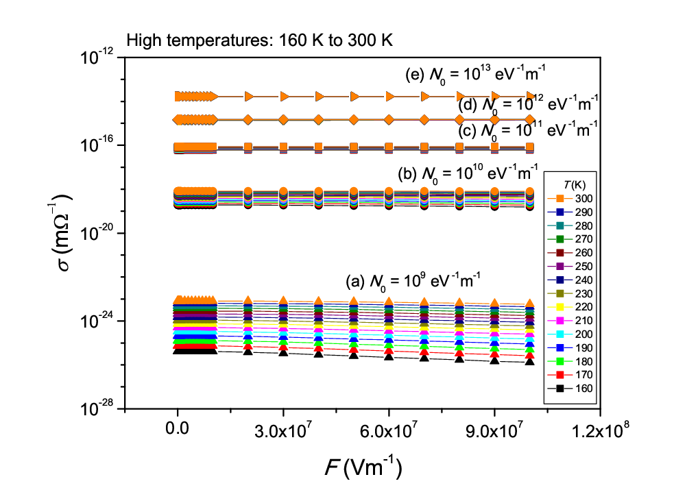
For the temperature range $T=(160$ - $300)$ K, Fig. 3 presents $\sigma$ as a function of $T^{-1/2}$ for different magnitudes of the DOS, i.e. for $N_{0}=(10^{9}$ - $10^{13})$ eV^-1m^-1 [cases (a) to (e), respectively]. $\alpha^{-1}=2$ $\AA$. $F=(5\times 10^{3}$ - $1\times 10^{8})$ Vm^-1. We depict our results as a function of $T^{-1/2}$ to compare them with the analytically obtained formula $\ln\sigma\propto T^{-1/2}$ which holds for low up to moderate electric fields and was previously obtained by two of us [26] following a different theoretical treatment and taking into account the effect of correlations, namely

Here $g(T)=\left(2\alpha k_{B}T/e\right)^{2}$ and $T_{0}^{h,cr}=1.18\alpha/k_{B}N_{0}$. We observe that higher density of states leads to higher conductivity in such a way that $\frac{d\sigma}{dN_{0}}$ is smaller for higher densities of states. As shown in Fig. 3, in this specific example, augmenting DOS by four orders of magnitude, the conductivity rises by approximately eleven orders of magnitude.

From these results we realize that the $T^{-1/2}$-behaviour of $\sigma$ [26] holds for low up to moderate electric fields. For the smaller densities of states, i.e. for $N_{0}=10^{9}$ and $10^{10}$ eV^-1m^-1, $\frac{d\sigma}{dF}<0$ i.e. the conductivity is larger for lower electric field strengths. This is due to the competitive role of the directionality imposed by the electric field and the temperature. This directionality affects destructively $\sigma$ when not many sites are available for the carrier i.e. for small densities of states. Here we notice that according to Eq. 16 and Fig. 1(I), the electric field affects the range between two sites in the “hopping space” both for the absorption and the emission branch. On the contrary, this effect does not appear at low temperatures ($T=(10$ - $150)$ K), discussed later on Subsection 3.2 (Fig. 8) because in the corresponding expression for the range between two sites in the “hopping space” at low temperatures (Eq. 27 and Fig. 2(I)), the electric field affects only the finite area of the absorption branch. We mention that the electric field plays a constructive role, too, due to its energy offer to the carriers. At $N_{0}=10^{11}$ eV^-1m^-1 it seems that the available sites are numerous enough so that the directionality of the electric field hardly affects the conductivity. For higher densities of states, i.e. for $N_{0}=10^{12}$ and $10^{13}$ eV^-1m^-1, only the constructive energetic influence of the electric field appears. Now $\frac{d\sigma}{dF}>0$ i.e. the conductivity is larger for higher electric field strengths. Finally, we observe that the temperature has a greater effect on the conductivity, the smaller the density of states is. Another aspect of the behaviour of the conductivity for different DOS is shown in Figure 4. $N_{0}=10^{9}$ - $10^{13}$ eV^-1m^-1, $T=(160$ - $300)$ K and $F=(5\times 10^{3}$ - $1\times 10^{8})$ Vm^-1.

Let us denote by $\sigma_{0}$ the ohmic value of the conductivity, i.e. $\sigma_{0}=\lim_{F\to 0}(\sigma)$. In order to show the deviation of $\sigma$ from $\sigma_{0}$ under the influence of both $F$ and $T$ we present Fig. 5 which shows $\sigma/\sigma_{0}$ versus $\beta=eF/2\alpha k_{B}T$ for (a) $N_{0}=10^{9}$ eV^-1m^-1 and (c) $N_{0}=10^{11}$ eV^-1m^-1, respectively. $F=(5\times 10^{3}$ - $1\times 10^{8})$ Vm^-1 and $T=(160$ - $300)$ K. We observe that the effect of the external stimuli $F$ and $T$ on $\sigma$ depends strongly on the value of the density of states that characterizes the system. For (a) $N_{0}=10^{9}$ eV^-1m^-1 the conductivity decreases from its ohmic value in the specific range of $F$ and $T$, while for (c) $N_{0}=10^{11}$ eV^-1m^-1 the conductivity generally increases and it is higher for higher temperatures. We notice that the variation of $\sigma/\sigma_{0}$ versus $\beta=eF/2\alpha k_{B}T$ is generally small especially in contrast to the corresponding variation at low temperatures studied later on Subsection 3.2.

Figure 6 shows the conductivity for different values of the spatial extent of the localized electronic wave function, i.e. for $\alpha^{-1}=(1$ - $5)$ $\AA$. Here we have chosen case (c) $N_{0}=10^{11}$ eV^-1m^-1 for the density of states. $T=(160$ - $300)$ K and $F=(5\times 10^{3}$ - $1\times 10^{8})$ Vm^-1. We observe that smaller $\alpha^{-1}$ (more localized carriers) leads to smaller $\sigma$. Particularly, five times increase of $\alpha^{-1}$ leads to two orders of magnitude greater conductivity. In addition, in Fig. 7 we observe that $\frac{d\sigma}{d\beta}>0$ for any temperature when $\alpha^{-1}=$ 3, 4 and 5 $\AA$, while $\frac{d\sigma}{d\beta}<0$ when $\alpha^{-1}=$ 1 $\AA$. For the case $\alpha^{-1}=$ 2 $\AA$ cf. Fig. 5(II). In other words, the strength of the localization which determines the size of the formed polaron, along with the density of states which characterizes the system, are both two key factors for the conductivity and its dependance on $F$ and $T$.

For the temperature range $T=(10$ - $150)$ K, Fig. 8 presents $\sigma$ as a function of $T^{-1/2}$ for different magnitudes of the DOS, i.e. $N_{0}=(10^{9}$ - $10^{11})$ eV^-1m^-1 [cases (a) to (c), respectively]. $\alpha^{-1}=2$ $\AA$. $F=(5\times 10^{3}$ - $1\times 10^{8})$ Vm^-1. Again, we depict our results as a function of $T^{-1/2}$ in order to compare them with the analytically obtained formula $\ln\sigma\propto T^{-1/2}$ which holds for low up to moderate electric fields and was previously obtained by two of us [26] following a different theoretical treatment and taking into account the effect of correlations, namely

Here $T_{0}^{l,cr}=1.96\alpha/k_{B}N_{0}$. We observe that higher density of states leads to higher conductivity in such a way that $\frac{d\sigma}{dN_{0}}$ is smaller for higher densities of states. In total, in this specific example, augmenting DOS by two orders of magnitude increases the conductivity by approximately tens of orders of magnitude. From these results we realize that the $T^{-1/2}$-behaviour of $\sigma$ [26] holds for low up to moderate electric fields. For higher values of $F$ the conductivity deviates from the $T^{-1/2}$-behaviour as $T$ decreases and this deviation appears to be larger the stronger the electric field is. This deviation is due to the constructive energetic contribution of the electric field which leads to the increase of the number of available sites that can host the carrier, i.e. the range $\overline{\Re}_{nn}^{l}$ does not depend solely on $T$. As the temperature further decreases, for strong enough electric fields, the range $\overline{\Re}_{nn}^{l}$ depends exclusively on the applied electric field, as essentially all hops are downward in energy. As a result, the conductivity does not depend on the temperature. In other words, there is a transition from thermally-assisted to field-assisted hopping.

We remind the reader that in the high temperature range $T=(160$ - $300)$ K discussed in subsection  3.1, the electric field affects the range between two sites in the “hopping space” both for the absorption and the emission branch, leading also to the appearance of the destructive role of the electric field. In contrast, this effect does not appear here in the low temperature range $T=(10$ - $150)$ K, because in the corresponding expression for the range between two sites in the “hopping space” the electric field affects only the finite area of the absorption branch.

Figure 9(I) presents the conductivity for different densities of states $N_{0}=10^{9}$ - $10^{11}$ eV^-1m^-1 as a function of the applied electric field. For low up to moderate electric fields the conductivity follows nicely the $F^{2}$-behaviour, as we expected from the analytical expression previously reported [24, 26]. Specifically, when the condition $F^{2}/g(T)\ll 1$ is satisfied, i.e. $e\alpha^{-1}F\ll 2k_{B}T$, two of us have showed [26]

where $\ln\sigma^{l,cr}(0,T)=-(T_{0}^{l,cr}/T)^{1/2}$, $h(F)=F^{2}$ and $f^{l,cr}(T)=[(T_{0}^{l,cr}/T)^{1/2}/2g(T)]^{-1}$. Increasing the electric field the conductivity becomes independent of the temperature and follows a $1/F^{1/2}$-behaviour (Fig. 9(II)). The linear fit is of the form $y=A+Bx$ with $A=-15.664\pm 0.018$, $B=-11159.837\pm 142.759$ and $R=-0.99959$. In the region between the $F^{2}$ and $1/F^{1/2}$-behaviour, $\ln\sigma$ increases almost linearly with $F$.

The influence of both $F$ and $T$ on $\sigma$ is shown in Fig. 10, where we depict $\sigma/\sigma_{0}$ versus $\beta=eF/2\alpha k_{B}T$, for (a) $N_{0}=10^{9}$ eV^-1m^-1 and (c) $N_{0}=10^{11}$ eV^-1m^-1. $F=(5\times 10^{3}$ - $1\times 10^{8})$ Vm^-1 and $T=(10$ - $150)$ K. The influence of $F$ on $\sigma$ depends on $T$, and it is greater at lower temperatures, while at higher temperatures the influence of $F$ decreases significantly. Comparing Fig. 10 with the corresponding one for high temperatures (cf. Fig. 5) we observe that the dependence of $\sigma/\sigma_{0}$ on $\beta=eF/2\alpha k_{B}T$ for low temperatures is very strong especially in contrast to the corresponding variation at high temperatures studied earlier on Subsection 3.1.

Fogler and Kelley [22], Raikh and Ruzin [25], and Ma et al. [23] refer also to the transition of a 1D disordered electron system from the ohmic to the non-ohmic behaviour, and in this respect their results are consistent with our results, for both low and high temperatures. For strong enough electric fields, Fogler and Kelley [22], Pollak and Riess [46], and Shklovskii [47], claim that in strong electric fields only the forward hops need to be considered, in contrast to Apsley and Hughes [40] who integrate over the entire space. Our methodology follows in that sense Apsley and Hughes [40] summing over forward as well as backward hops in our 1D polaron system. Bourbie et al. [48] study the $F$-dependence of the hopping conductivity in disordered 3D electron systems. They propose –among other mechanisms– that $\sigma$ decreases with increasing $F$, when $F$ is strong enough to affect the tunneling probability. This is due to the influence of $F$ on the number of percolation paths, in the sense that increasing $F$ certain paths become disallowed. This is in analogy with our discussion about the destructive role of $F$ at high $F$ and low DOS. Bourbie et al. [29], taking into account that “$F$ affects the effective dimension of the transport path, reducing it in the high-$F$ regime to 1D”, showed that when $F=10^{8}$ Vm^-1, $T\approx$ (200 - 330) K, $\alpha^{-1}=$ 2 $\AA$ and $N_{0}=10^{12}$ eV^-1m^-1, the conductivity decreases with increasing temperature. This has been attributed to the competition between thermal-assisted and field-assisted hopping. We have obtained a similar behaviour for $\sigma$ when $F=10^{8}$ Vm^-1, at high temperatures $T=$ (160-300) K, $\alpha^{-1}=$ 2$\AA$ and $N_{0}=10^{13}$ eV^-1m^-1 (cf. Fig. 3). Bourbie et al. have also included different forms of the DOS and mention that these different DOS lead to very similar $F$-dependence of $\sigma$. D. Bourbie [30] also used some different values for the extent of the 3D electronic wave function arriving at the result that greater extent of the carrier leads to higher conductivity in analogy with our results for 1D polarons. However, we underline that all the above works [22, 40, 46, 47, 48, 29, 30] refer to electrons while we study polarons. Moreover, in our work we have scrutinized the importance of the magnitude of the density of states and the spatial extent of the localized electronic wave function (for arbitrary electric fields up to the polaron dissociation limit and for any “reasonable” temperature). Finally, in 1D systems the ionic or protonic transport might play a role in some cases [49, 50, 51, 52]. However, in the present manuscript we do not investigate such possibilities.

References

- [1] Gleve B, Hartenstein B, Baranovskii S D, Scheidler M, Thomas P and Bössler H 1995 Phys. Rev. B 51 16705
- [2] Nebel C E, Street R A, Johnson N M and Kocka J 1992 Phys. Rev. B 46 6789
- [3] Godet C and Kumar S 2003 Phil. Mag. 83 3351
- [4] Cumings J and Zettl A 2004 Phys. Rev. Lett. 93 086801
- [5] Tang Z K, Sun H D and Wang J 2000 Physica B 279 200
- [6] Campbell I H, Smith D L, Neef C J and Ferraris J P 1999 Appl. Phys. Lett. 74 2809
- [7] Mozer A Z, Sariciftci N S, Pivrikas A, Österbacka R, Juska G, Brassat L and Bässler” H 2005 Phys. Rev. B 71 035214
- [8] Novikov S V, Dunlap D H, Kenkre V M, Parris P E and Vannikov A V 1998 Phys. Rev. Lett. 81 4472
- [9] Aleshin A N, Lee J Y, Chu S W, Lee S W, Kim B, Ahn S J and Park Y W 2004 Phys. Rev. B 69 214203
- [10] Yu Z G, Smith D L, Saxena A, Martin R L and Bishop A R 2000 Phys. Rev. Lett. 84 721
- [11] Yu Z G, Smith D L, Saxena A, Martin R L and Bishop A R 2001 Phys. Rev. B 63 085202
- [12] Triberis G. P. and Dimakogianni M 2009 Rec. Pat. Nanotechnol. 3 135
- [13] Triberis G P, Simserides C and Karavolas V C 2005 J. Phys.: Condens. Matter 17 2681
- [14] Triberis G P and Friedman L R 1981 J. Phys. C.: Solid State Phys. 14 4631
- [15] Tran P, Alavi B and Gruner G 2000 Phys. Rev. Lett. 85 1564
- [16] Yoo K-H, Ha D H, Lee J-O, Park J W, Kim J, Kim J J, Lee H-Y, Kawai T and Choi H-Y 2001 Phys. Rev. Lett. 87 198102
- [17] Triberis G P and Dimakogianni M 2009 J. Phys.: Condens. Matter 21 035114
- [18] Inomata A, Shimomura T, Heike S, Fujimori M, Hashizume T and Ito K 2006 J. Phys. Soc. Japan 75 074803
- [19] Schuster G B 2000 Acc. Chem. Res. 33 253
- [20] Carell T, Behrens C and Gierlich J 2003 J. Org. Biomol. Chem. 1 2221
- [21] Takada T, Kawai K, Fujitsuka M and Majima T 2004 Natl. Acad. Sci. (USA) 101 14002
- [22] Fogler M M and Kelley R S 2005 Phys. Rev. Lett. 95 166604
- [23] Ma S, Xu H, Li Y and Song Z 2007 Physica B 398 55
- [24] Triberis G P and Dimakogianni M 2009 J. Phys.: Condens. Matter 21 385406
- [25] Raikh M E and Ruzin I M 1989 Sov. Phys. JETP 68 642
- [26] Dimakogianni M and Triberis G P 2010 J. Phys.: Condens. Matter 22 355305
- [27] Hawke L G D, Kalosakas G and Simserides C 2010 Eur. Phys. J. E 32 291
- [28] Hawke L G D, Kalosakas G and Simserides C 2011 Eur. Phys. J. E 34 118
- [29] Bourbie D, Ikrelef N, Driss-Khodja K and Nedellec P 2007 Phys. Rev. B 75 184204
- [30] Bourbie D 2011 Appl. Phys. Lett. 98 012104
- [31] Hawke L G D, Kalosakas G and Simserides C 2009 Mol. Phys. 107 1755
- [32] Hawke L G D, Simserides C and Kalosakas G 2009 Mater. Sci. Eng. B 165 266
- [33] Triberis G P and Friedman L R 1986 J. Non-Crystalline Solids 79 29
- [34] Emin D 1975 Adv. Phys. 24 305
- [35] Triberis G P 1985 Phys. Stat. Sol. (b) 132 641
- [36] Kubo R 1957 J. Phys. Soc. Japan 12 1203
- [37] Ambegaokar V, Halperin B I and Langer J S 1971 Phys. Rev. B 4 2612
- [38] Emin D 1975 Phys. Rev. Lett. 35 882
- [39] Fehske H and Trugman S A 2007 Numerical Solution of the Holstein Polaron Problem p 396 in Polarons in Advanced Materials (ed Alexandrov A S) (Springer)
- [40] Apsley N and Hughes H P 1975 Phil. Mag. 31 1327
- [41] Triberis G P, Zianni X, Yannacopoulos A N and Karavolas V C 1991 J. Phys. Condens. Matter 3 337
- [42] Triberis G P 1992 Phil. Mag. 65 631
- [43] Rakhmanova S V and Conwell E M 1999 Appl. Phys. Lett. 75 1518
- [44] Liu X, Gao K, Fu J, Li Y, Wei J and Xie S 2006 Phys. Rev. B 74 172301
- [45] Qiu Y and Zhu L-P 2009 J. Chem. Phys. 131 134903
- [46] Pollak M and Riess I 1976 J. Phys. C.: Solid State Phys. 9 2339
- [47] Shklovskii B I 1973 Sov. Phys. Semicond. 6 1964
- [48] Bourbie D, Ikrelef N and Nedellec P 2004 Phys. Stat. Sol. (c) 1 79
- [49] Wang J 2008 Phys. Rev. B 78 245304
- [50] Pavlenko N 2000 J. Chem. Phys. 112 8637
- [51] Pavlenko N 2003 J. Phys.: Condens. Matter 15 291
- [52] Rak J, Makowska J, Voityuk A A 2006 Chemical Physics 325 567