跳到论文正文
W Papers独立论文阅读器 arXiv:1209.1569 论文正文 计算阅读时间 · 0%
引用这篇论文根据当前论文元数据生成,正式投稿前建议核对。


License: arXiv.org perpetual non-exclusive license
arXiv:1209.1569v3 [hep-ph] 28 May 2013

Nagy-Soper subtraction scheme
for multiparton final states

Cheng-Han Chung
Supercomputing Research Center, National Cheng Kung University,
Tainan 701, Taiwan

Tania Robens
IKTP, TU Dresden, Zellescher Weg 19, 01069 Dresden, Germany

Abstract:
In this work, we present the extension of an alternative subtraction scheme for next-to-leading order QCD calculations to the case of an arbitrary number of massless final-state partons. The scheme is based on the splitting kernels of an improved parton shower and comes with a reduced number of final state momentum mappings. While a previous publication including the setup of the scheme has been restricted to cases with maximally two massless partons in the final state, we here provide the final state real emission and integrated subtraction terms for processes with any number of massless partons. We apply our scheme to three jet production at lepton colliders at next-to-leading order and present results for the differential C parameter distribution.

1 Introduction

With the start of data taking at the LHC in 2009 and its more than successful physics program since then, particle physics has entered an exciting era. Major tasks of the LHC experiments are the accurate measurement of the parameters of the Standard Model (SM) of particle physics, as well as the search for physics beyond the SM. For both, a precise understanding of the SM signals and background processes in an hadronic environment are crucial. These processes are mainly governed by strong interactions, where leading order (LO) calculations can exhibit uncertainties up to 100%100\,\% (c.f. [1] for a recent review); therefore, for a correct theoretical prediction of these processes at least next-to-leading order (NLO) corrections need to be taken into account. Furthermore, it is generally not sufficient to apply an overall NLO rescaling K-factor to the leading order predictions, as NLO corrections can vary widely for different regions of phase space. More accurate predictions therefore call for the inclusion of these NLO calculations in Monte Carlo event generators, which provide predictions for fully differential corrections to the LO process. Many such generators exist at parton level [2, 3, 4, 5, 6, 7, 8, 9, 10, 11, 12, 13, 14, 15, 16, 17, 18], and in recent years a lot of progress has equally been made to automatize the matching of these processes with parton showers in the Powheg[19, 20, 21, 22, 23, 24, 25, 26, 27, 28, 29, 30, 31, 32, 33, 34, 35, 36, 37, 38, 39, 40] and (a)MC@NLO [41, 22, 42, 43, 44, 45, 46, 47, 48, 49] frameworks11 1 Recent reviews on this can be found in [50, 51]..

In this paper, we present the generic extension of an improved subtraction scheme[52, 53, 54], which facilitates the inclusion of infrared (IR) NLO divergences originating from different phase space contributions in Monte Carlo event generators. These divergences arise whenever internal loop momenta approach zero or particles become collinear, and are known to cancel in any fixed order in perturbation theory [55, 56]. However, these cancellations occur in the combined sum of virtual and real emission contributions, and therefore originate from phase spaces with a different number of particles in the final state. In analytic or semi-numerical calculations, the singularities can be parametrized by an infinitesimal regulator; in the sum of real and virtual contributions, these regulators can then be set to zero to obtain a completely finite prediction. In numerical implementations, however, the inclusion of infinitesimal regulators can easily lead to numerical instabilities. Subtraction methods[57, 58, 59, 60, 61, 62, 63, 64, 65, 66] circumvent this problem by introducing local counterterms that mimic the behaviour of the real emission matrix elements in the singular limits. The integrated counterparts of these terms are then added to the virtual contributions, where again an infinitesimal regulator is used to parametrize the singularities. Then, the higher order contributions in both phase space integrations are finite, and the regulator can be set to zero. In recent years, many of these schemes have been made available on a (semi)automated level [67, 65, 68, 69, 70, 26].

While the behaviour of the subtraction terms in the singular limit is determined by factorization [71, 72, 73], the finite parts of the local counterterms as well as the mapping prescription between real emission and leading order phase space kinematics in the subtraction terms can differ. Unfortunately, standard schemes [59, 64] suffer from a rapidly rising number of momentum mappings, which scales like N3N^{3} for a leading order 2→N2\,\rightarrow\,N process. Therefore, increasing the number of final state particles leads to a rapidly rising number of reevaluations of the Born matrix element. In [52, 53, 54], we therefore proposed a new subtraction scheme with a modified momentum mapping [74, 75, 76], where the number of momentum mappings scales as ∼N2\sim\,N^{2}. The momentum mappings are constructed such that they take the whole remaining event as a spectator, and the subtraction terms are derived from the splitting functions in an improved parton shower[74, 75, 76]. In [52, 53, 54], we presented the scheme for the simplest cases with maximally two partons in the final state22 2 Some results for the generic scheme were already presented in [52].. In the present work, we extend the scheme to cases with an arbitrary number of massless particles in the final state. We also provide the helicity dependent squared splitting functions for splittings where the mother parton is a gluon. We validate our scheme by applying it to three-jet production at NLO at lepton colliders, obtaining complete agreement with the Catani Seymour scheme.

This paper is organized as follows. In Section 2, we briefly review the generic setup for subtraction schemes. In Section 3, we review the ingredients of the new scheme and present the generalized results for the integrated subtraction terms for an arbitrary number of final state massless partons. We discuss the application of our scheme to three-jet production at lepton colliders in Section 4. Conclusion and outlook are presented in Section 5. The Appendix contains a summary of the final state splitting functions [74] used as subtraction terms, a generic parametrization of four-parton phase space, and the collinear subtraction terms for processes with incoming hadrons.

2 General structure of NLO cross sections and subtraction schemes

In this section, we briefly review the general subtraction procedure for calculating NLO cross sections at lepton and hadron colliders. We start with a generic cross section at NLO

σ\displaystyle\sigma =\displaystyle= ∫md​σB⏟σLO+∫m+1d​σR+∫md​σV⏟σNLO\displaystyle\underbrace{\int_{m}d\sigma^{B}}_{\sigma^{\text{LO}}}\,+\,\underbrace{\int_{m+1}d\sigma^{R}\,+\,\int_{m}d\sigma^{V}}_{\sigma^{\text{NLO}}} (1)

where σ\sigma should be specified by the respective jet function as discussed below, and d​σB,d​σR,d\sigma^{B},\,d\sigma^{R}, and d​σVd\sigma^{V} are the Born, real emission, and virtual contribution respectively. We here consider processes with mm particles in the Born-contribution and m+1m+1 partons in the real emission terms. After UV-renormalisation, the virtual and real-emission cross sections each contain infrared and collinear singularities. These cancel in the sum of virtual and real contributions[55, 56], but the individual pieces are divergent and can therefore not be integrated numerically in four dimensions.

Subtraction schemes consist of local counterterms that match the behaviour of the real-emission matrix element in the soft and collinear regions, and their integrated counterparts. Subtracting these counterterms from the real-emission matrix elements and adding back the integrated counterparts to the virtual contribution results in finite integrands for both the virtual correction (mm-particle phase space) and the real contribution ((m+1CLOSE(m+1)-particle phase space):

d​σNLO=[d​σR−d​σA]+[d​σA+d​σV].d\sigma^{\text{NLO}}\,=\,\left[d\sigma^{R}-d\sigma^{A}\right]\,+\,\left[d\sigma^{A}\,+\,d\sigma^{V}\right]. (2)

The construction of the local counterterms, collectively denoted by d​σAd\sigma^{A}, relies on the factorisation of the real-emission matrix element in the singular (i.e. soft and collinear) limits (Fig. 1) [71, 72, 73], and we symbolically write

 Refer to caption
Figure 1: Soft/collinear factorisation: when the partons ℓ\ell and jj become collinear and/or parton jj becomes soft, the (m+1m+1)-parton matrix element factorises into a sum over mm-parton matrix elements times a singular factor vℓ{v}_{\ell}.
 
|ℳm+1​(p^)|2⟶𝒟ℓ⊗|ℳm​(p)|2,\left|{\cal M}_{m+1}(\hat{p})\right|^{2}\quad\longrightarrow\quad\mathcal{D}_{\ell}\,\otimes\,\left|{\cal M}_{m}(p)\right|^{2}, (3)

where 𝒟ℓ\mathcal{D}_{\ell} are the dipoles containing the respective singularity structure, and the symbol ⊗\otimes denotes a correct convolution in color, spin, and flavour space. p^/p\hat{p}/\,p represent momenta in (m+1)/m(m+1)/\,m-parton phase space, respectively. As |ℳm+1|2\left|{\cal M}_{m+1}\right|^{2} and |ℳm|2\left|{\cal M}_{m}\right|^{2} live in different phase spaces, a mapping of their momenta needs to be introduced, which is defined by a mapping function FmapF_{\textrm{map}} according to

p=Fmap​(p^).{p}\,=\,F_{\textrm{map}}\,(\hat{p}). (4)

𝒟ℓ\mathcal{D}_{\ell} and its one-parton integrated counterpart 𝒱ℓ\mathcal{V}_{\ell} are related by

𝒱ℓ=∫d​ξp​𝒟ℓ,\mathcal{V}_{\ell}\,=\,\int\,d\xi_{p}\,\mathcal{D}_{\ell}, (5)

where d​ξpd\xi_{p} is an unresolved one parton integration measure.

In summary, any subtraction scheme needs to fulfill the following requirements:

  • •

    The dipole subtraction terms 𝒟ℓ\mathcal{D}_{\ell} must match the behaviour of the real emission matrix element in each soft and collinear region, and lead to correct IR poles when carrying out the analytical integration over the one parton phase space in a suitable regularization scheme that are necessary to cancel the soft singularities in the virtual (one-loop) matrix element,

  • •

    The mapping function FmapF_{\textrm{map}} guarantees total energy momentum conservation as well as the on-shell condition for all external particles before and after the mapping.

Integrating Eqn. (2) over phase space using dimensional regularization[77, 78], where D= 4−2​εD\,=\,4-2\,\varepsilon, then yields

σNLO\displaystyle\sigma^{\text{NLO}} =\displaystyle= ∫m+1[d​σR−d​σA]⏟finite+∫m+1d​σA+∫md​σV⏟finite\displaystyle\underset{\textrm{finite}}{\underbrace{\int_{m+1}\left[d\sigma^{R}-d\sigma^{A}\right]}}+\underset{\textrm{finite}}{\underbrace{\int_{m+1}\,d\sigma^{A}+\int_{m}\,d\sigma^{V}}} (6)
=\displaystyle= ∫m+1[d​σε=0R−d​σε=0A]+∫m[∫1d​σA+d​σV]ε=0.\displaystyle\int_{m+1}\left[d\sigma^{R}_{\varepsilon=0}-d\sigma^{A}_{\varepsilon=0}\right]+\int_{m}\left[\int_{1}\,d\sigma^{A}+d\sigma^{V}\right]_{\varepsilon=0}.

Both integrands are now finite: the integration in (m+1CLOSE(m+1) particle phase space can safely be performed in D= 4D\,=\,4 dimensions, as the singular regions are regularized by the respective counterterms. In the mm parton phase space, the sum of the integrated dipole contribution and the virtual correction does not contain any further poles, so that we can set ε=0\varepsilon=0. Then, all integrations can be performed numerically. The explicit expressions of the cross section σ\sigma for mm and (m+1CLOSE(m+1) particle phase space contributions at NLO are

∫m[d​σB+d​σV+∫1d​σA]\displaystyle\int_{m}\,\left[d\sigma^{B}\,+\,d\sigma^{V}\,+\,\int_{1}\,d\sigma^{A}\right] =∫d​P​Sm​[|ℳm|2+|ℳm|one-loop2+∑ℓ𝒱ℓ⊗|ℳm|2],\displaystyle=\int dPS_{m}\left[\left|{\cal M}_{m}\right|^{2}\,+\,\left|{\cal M}_{m}\right|^{2}_{\textrm{one-loop}}\,+\,\sum_{\ell}\,\mathcal{V}_{\ell}\,\otimes\,\left|{\cal M}_{m}\right|^{2}\right],
∫m+1[d​σR−d​σA]\displaystyle\int_{m+1}\,\left[d\sigma^{R}-d\sigma^{A}\right] =∫d​P​Sm+1​[|ℳm+1|2−∑ℓDℓ⊗|ℳm|2],\displaystyle=\int dPS_{m+1}\left[\left|{\cal M}_{m+1}\right|^{2}\,-\,\sum_{\ell}\,D_{\ell}\,\otimes\,\left|{\cal M}_{m}\right|^{2}\right], (7)

where in this symbolic notation ∫d​P​S\int dPS includes all flux and symmetry factors, and with |ℳm|2\left|{\cal M}_{m}\right|^{2}, |ℳm+1|2\left|{\cal M}_{m+1}\right|^{2} and |ℳm|one-loop2\left|{\cal M}_{m}\right|^{2}_{\textrm{one-loop}} being the squared LO matrix element, the squared real emission matrix element and the interference term, respectively. In Eqn. (7), the sum runs over all local counterterms needed to match the complete singularity structure of the real emission contribution, and convolution with jet functions then ensures the collinear and infrared safety of the Born-level contribution. The insertion operator I⁡(ε)I(\varepsilon) is then defined on a cross section level according to

∫m∫1d​σA=∫md​σB⊗I⁡(ε),\int_{m}\int_{1}d\sigma^{A}=\int_{m}d\sigma^{B}\otimes{I}(\varepsilon),

where the symbol ⊗\otimes again denotes a proper convolution in spin, color, and phase space. The generalization of this for processes with initial state hadrons has already been presented in [53]; for completeness, we repeat the argument in Appendix B.

Observable-dependent formulation of the subtraction method

The jet observables should be well defined such that the leading order cross sections are infrared and collinear safe. The jet cross sections are defined as

σJL​O\displaystyle\sigma^{LO}_{J} =∫d​P​Sm​(p1,⋯,pm)​|ℳm​(p1,⋯,pm)|2​FJ(m)​(p1,⋯,pm),\displaystyle=\int dPS_{m}(p_{1},\cdots,p_{m})\,\left|{\cal M}_{m}(p_{1},\cdots,p_{m})\right|^{2}\,F_{J}^{(m)}(p_{1},\cdots,p_{m}),
σJN​L​O\displaystyle\sigma^{NLO}_{J} =∫d​P​Sm+1​(p1,⋯,pm+1)​|ℳm+1​(p1,⋯,pm+1)|2​FJ(m+1)​(p1,⋯,pm+1)\displaystyle=\int dPS_{m+1}(p_{1},\cdots,p_{m+1})\,\left|{\cal M}_{m+1}(p_{1},\cdots,p_{m+1})\right|^{2}\,F_{J}^{(m+1)}(p_{1},\cdots,p_{m+1})
+∫dPSm(p1,⋯,pm)|ℳm(p1,⋯,pm)|one-loop2FJ(m)(p1,⋯,pm).\displaystyle+\int dPS_{m}(p_{1},\cdots,p_{m})\,\left|{\cal M}_{m}(p_{1},\cdots,p_{m})\right|^{2}_{\textrm{one-loop}}\,F_{J}^{(m)}(p_{1},\cdots,p_{m}). (8)

In general, the jet function may contain θ\theta functions (which define cuts and corresponding cross sections) and δ\delta functions (which define differential cross sections). For an infrared finite jet function, we require that

FJ(m+1)​(p1,⋯,pj=λ​q,⋯,pm+1)\displaystyle F_{J}^{(m+1)}(p_{1},\cdots,p_{j}=\lambda\,q,\cdots,p_{m+1}) →\displaystyle\to FJ(m)​(p1,⋯,pm+1),ifλ→0\displaystyle F_{J}^{(m)}(p_{1},\cdots,p_{m+1}),\quad{\textrm{if}}\quad\lambda\to 0
FJ(m+1)(p1,..,pi,..,pj,..,pm+1)\displaystyle F_{J}^{(m+1)}(p_{1},..,p_{i},..,p_{j},..,p_{m+1}) →\displaystyle\to FJ(m)(p1,..,p,..,pm+1)\displaystyle F_{J}^{(m)}(p_{1},..,p,..,p_{m+1})
ifpi→z​p,pj→(1−z)​p,\displaystyle\quad\quad\quad\quad{\textrm{if}}\quad p_{i}\to z\,p,\,p_{j}\to(1-z)\,p,
FJ(m)​(p1,⋯,pm)\displaystyle F_{J}^{(m)}(p_{1},\cdots,p_{m}) →\displaystyle\to 0,ifpi⋅pj→0.\displaystyle 0,\quad{\textrm{if}}\quad p_{i}\cdot p_{j}\to 0. (9)

The last condition of Eqn. (9) corresponds to an infrared safe definition of the Born-level observable, while the first two conditions guarantee infrared and collinear safety of the observables and can be summarized to

FJ(m+1)→FJ(m)F_{J}^{(m+1)}\,\to\,F_{J}^{(m)} (10)

in the singular limits.

We then have

∫m[d​σB+d​σV+∫1d​σA]\displaystyle\int_{m}\,\left[d\sigma^{B}\,+\,d\sigma^{V}\,+\,\int_{1}\,d\sigma^{A}\right]
=\displaystyle= ∫d​P​Sm​[|ℳm|2+|ℳm|one-loop2+∑ℓ𝒱ℓ⊗|ℳm|2]​FJ(m)​(p),\displaystyle\int dPS_{m}\left[\left|{\cal M}_{m}\right|^{2}\,+\,\left|{\cal M}_{m}\right|^{2}_{\textrm{one-loop}}\,+\,\sum_{\ell}\,\mathcal{V}_{\ell}\,\otimes\,\left|{\cal M}_{m}\right|^{2}\right]\,F_{J}^{(m)}(p),
∫m+1[d​σR−d​σA]\displaystyle\int_{m+1}\,\left[d\sigma^{R}-d\sigma^{A}\right]
=\displaystyle= ∫d​P​Sm+1​[|ℳm+1|2​FJ(m+1)​(p^)−∑ℓ𝒟ℓ⊗|ℳm|2​FJ(m)​(p)],\displaystyle\int dPS_{m+1}\,\left[\left|{\cal M}_{m+1}\right|^{2}\,F_{J}^{(m+1)}(\hat{p})\,-\,\sum_{\ell}\,\mathcal{D}_{\ell}\,\otimes\,\left|{\cal M}_{m}\right|^{2}F_{J}^{(m)}(p)\right],

where in the integrated subtraction term the momenta pp are derived from p^\hat{p} using the respective momentum mapping.

3 Alternative subtraction scheme: setup

In this section, we will first review the setup of our scheme as well as the mapping and respective integration measures which have already been presented in [74, 53]. In our scheme, the NLO subtraction terms are derived from the splitting functions introduced in a parton shower context [74, 75, 76], and the m+1m+1 to mm phase space mappings needed correspond to the inverse of the respective shower mm to m+1m+1 mappings. In the following, we will denote the m+1m+1 phase space four-vectors by p^1,p^2,…\hat{p}_{1},\hat{p}_{2},... and mm phase space four-vectors by p1,p2,…p_{1},\,p_{2},\,.... In m+1m+1 phase space, the four-momenta of the emitter, emitted particle, and spectator are denoted p^ℓ,p^j,\hat{p}_{\ell},\,\hat{p}_{j}, and p^k\hat{p}_{k} respectively. Note that here the spectator needs to be specified only if p^j\hat{p}_{j} denotes a gluon, as we use the whole remaining event as a spectator in the sense of momentum redistribution for both initial and final state mappings. We here restrict our expressions to subtractions on the parton level and to massless partons.

3.1 Splitting functions

We start with a description of the matrix element factorization in the soft and collinear limits, following the notation in [74], where the QCD scattering amplitude for m+1m+1 partons is given as a vector in (colour ⊗\otimes spin) space,

∣ℳ⁡({p^,f^}m+1)⟩.\mid{\cal M}(\{\hat{p},\hat{f}\}_{m+1})\rangle. (12)

In the singular limits, the amplitude ∣ℳℓ​({p^,f^}m+1)⟩\mid{\cal M}_{\ell}(\{\hat{p},\hat{f}\}_{m+1})\rangle can be factorized into a splitting operator times the mm-parton matrix element

∣ℳℓ​({p^,f^}m+1)⟩=tℓ†​(fℓ→f^ℓ+f^j)​Vℓ†​({p^,f^}m+1)​∣ℳ⁡({p,f}m)⟩,\mid{\cal M}_{\ell}(\{\hat{p},\hat{f}\}_{m+1})\rangle\,=\,t^{\dagger}_{\ell}(f_{\ell}\to\hat{f}_{\ell}+\hat{f}_{j})\,V^{\dagger}_{\ell}(\{\hat{p},\hat{f}\}_{m+1})\,\mid{\cal M}(\{p,f\}_{m})\rangle, (13)

where the index ℓ\ell labels the emitter/ mother parton in the (m+1CLOSE(m+1)/ mm particle phase space. Vℓ†​({p^,f^}m+1)V^{\dagger}_{\ell}(\{\hat{p},\hat{f}\}_{m+1}) is an operator acting on the spin part of the (colour ⊗\otimes spin) space, while tℓ†​(fℓ→f^ℓ+f^j)t^{\dagger}_{\ell}(f_{\ell}\to\hat{f}_{\ell}+\hat{f}_{j}) is an operator acting on the colour part of the (colour ⊗\otimes spin) space. The Born amplitude for producing mm partons is evaluated at momenta and flavours {p,f}m\{p,f\}_{m} determined from {p^,f^}m+1\{\hat{p},\hat{f}\}_{m+1} according to the respective momentum mappings. The spin-dependent splitting operator can be described in the spin space ∣{s}m⟩\mid\{s\}_{m}\rangle:

⟨{s^}m+1∣Vℓ†​({p^,f^}m+1)∣{s}m⟩.\langle\{\hat{s}\}_{m+1}\mid V^{\dagger}_{\ell}(\{\hat{p},\hat{f}\}_{m+1})\mid\{s\}_{m}\rangle. (14)

If we take Eqn. (14) to be diagonal, we can define the splitting functions vℓv_{\ell} according to

⟨{s^}m+1∣Vℓ†​({p^,f^}m+1)∣{s}m⟩=(∏n∉{ℓ,j=m+1}δs^n,sn)​vℓ​({p^,f^}m+1,s^j,s^ℓ,sℓ).\displaystyle\langle\{\hat{s}\}_{m+1}\mid V^{\dagger}_{\ell}(\{\hat{p},\hat{f}\}_{m+1})\mid\{s\}_{m}\rangle\,=\,\left(\prod_{n\notin\{\ell,j=m+1\}}\delta_{\hat{s}_{n},s_{n}}\right)\,v_{\ell}(\{\hat{p},\hat{f}\}_{m+1},\hat{s}_{j},\hat{s}_{\ell},s_{\ell}). (15)

Explicit forms for the splitting functions vℓv_{\ell} have been presented in [74]. For the construction of the subtraction terms, we consider the approximation for the squared matrix element in the singular limits

∑ℓ,ℓ′⟨ℳℓ({p^,f^}m+1|ℳℓ′({p^,f^}m+1⟩∼∑ℓ,ℓ′vℓ∗vℓ′⟨ℳ({pℓ,f}m)|ℳ({pℓ′,f}m)⟩.\sum_{\ell,\ell^{\prime}}\,\langle{\cal M}_{\ell}(\{\hat{p},\hat{f}\}_{m+1}|{\cal M}_{\ell^{\prime}}(\{\hat{p},\hat{f}\}_{m+1}\rangle\,\sim\,\sum_{\ell,\ell^{\prime}}\,\,v^{*}_{\ell}v_{\ell^{\prime}}\langle{\cal M}(\{p_{\ell},f\}_{m})|{\cal M}(\{p_{\ell^{\prime}},f\}_{m})\rangle.

For the direct splitting function, where ℓ=ℓ′\ell\,=\,\ell^{\prime}, we obtain

Wℓ​ℓ≡vℓ2=vℓ​({p^,f^}m+1,s^j,s^ℓ,sℓ)​vℓ∗​({p^,f^}m+1,s^j,s^ℓ,sℓ),W_{\ell\ell}\,\equiv\,v^{2}_{\ell}\,=\,v_{\ell}(\{\hat{p},\hat{f}\}_{m+1},\hat{s}_{j},\hat{s}_{\ell},s_{\ell})\,v^{*}_{\ell}(\{\hat{p},\hat{f}\}_{m+1},\hat{s}_{j},\hat{s}_{\ell},s_{\ell}), (16)

which, after summing over the daughter parton spins and averaging over the mother parton spins, leads to the spin-averaged splitting functions W¯ℓ​ℓ\overline{W}_{\ell\ell} as subtraction terms. If the mother parton is a gluon, the Born-type matrix element might have an explicit dependence on the gluons polarization; in this case, we need to use

⟨ν|Wℓ​ℓ|ν′⟩\langle\nu|W_{\ell\ell}|\nu^{\prime}\rangle (17)

in the real-emission subtraction terms, where ν,ν′\nu,\,\nu^{\prime} are the polarisation indices of the mm-parton phase space gluon. If the spin correlation tensor defined by Eqn. (17) is perpendicular to pℓp_{\ell}, the angular correlations vanish after the integration over the unresolved particles phase space and the integral over W¯ℓ​ℓ\overline{W}_{\ell\ell} still provides the correct integrated counterterm [59]. For the collinear terms, the colour factors can easily be obtained [74]:

C⁡(f^ℓ,f^j)={CF(f^ℓ,f^j)=(q,g),(g,q),CA(f^ℓ,f^j)=(g,g),TR(f^ℓ,f^j)=(q,q¯).\displaystyle C(\hat{f}_{\ell},\hat{f}_{j})\,=\,\begin{cases}C_{F}&(\hat{f}_{\ell},\hat{f}_{j})\,=\,(q,g),(g,q),\\ C_{A}&(\hat{f}_{\ell},\hat{f}_{j})\,=\,(g,g),\\ T_{R}&(\hat{f}_{\ell},\hat{f}_{j})\,=\,(q,\bar{q}).\\ \end{cases}

For soft gluon emissions, we also have to consider terms for which ℓ≠ℓ′\ell\,\neq\,\ell^{\prime}, which we will describe below.

3.1.1 Eikonal factor

When a gluon with four-vector p^j\hat{p}_{j} becomes soft, or soft and collinear with p^ℓ\hat{p}_{\ell}, the splitting amplitude vℓv_{\ell} defined in Eqn. (15) can be replaced by the eikonal approximation for p^j→ 0\hat{p}_{j}\,\rightarrow\,0

vℓeik​({p^,f^}m+1,s^j,s^ℓ,sℓ)=4​π​αs​δs^ℓ,sℓ​ε​(p^j,s^j,Q^)∗⋅p^ℓp^j⋅p^ℓ,v_{\ell}^{\textrm{eik}}(\{\hat{p},\hat{f}\}_{m+1},\hat{s}_{j},\hat{s}_{\ell},s_{\ell})\,=\,\sqrt{4\pi\alpha_{s}}\,\delta_{\hat{s}_{\ell},s_{\ell}}\,\frac{\varepsilon(\hat{p}_{j},\hat{s}_{j},\hat{Q})^{*}\cdot\hat{p}_{\ell}}{\hat{p}_{j}\cdot\hat{p}_{\ell}}, (18)

where ε⁡(p^j,s^j,Q^)\varepsilon(\hat{p}_{j},\hat{s}_{j},\hat{Q}) denotes the polarization vector of the emitted gluon with spin sjs_{j}. Q^\hat{Q} denotes the total momentum of the (m+1)(m+1) phase space event and is used as a gauge vector. The eikonal approximation of the spin-averaged splitting functions W¯ℓ​ℓ\overline{W}_{\ell\ell} is then

W¯ℓ​ℓeik= 4​π​αs​p^ℓ⋅D⁡(p^j,Q^)⋅p^ℓ(p^j⋅p^ℓ)2,\overline{W}_{\ell\ell}^{\textrm{eik}}\,=\,4\,\pi\,\alpha_{s}\,\frac{\hat{p}_{\ell}\cdot D(\hat{p}_{j},\hat{Q})\cdot\hat{p}_{\ell}}{(\hat{p}_{j}\cdot\hat{p}_{\ell})^{2}}, (19)

where flavour-dependent averaging factors are already taken into account. The transverse projection tensor Dμ​νD^{\mu\nu} is given by

Dμ​ν​(p^j,Q^)=−gμ​ν+p^jμ​Q^ν+Q^μ​p^jνp^j⋅Q^−Q^2​p^jμ​p^jν(p^j⋅Q^)2.D^{\mu\nu}(\hat{p}_{j},\hat{Q})\,=\,-g^{\mu\nu}+\frac{\hat{p}_{j}^{\mu}\,\hat{Q}^{\nu}+\hat{Q}^{\mu}\,\hat{p}_{j}^{\nu}}{\hat{p}_{j}\cdot\hat{Q}}-\frac{\hat{Q}^{2}\,\hat{p}_{j}^{\mu}\,\hat{p}_{j}^{\nu}}{(\hat{p}_{j}\cdot\hat{Q})^{2}}.

It will be convenient to define a dimensionless function FF:

F=p^ℓ⋅p^j4​π​αs​W¯ℓ​ℓ.F\,=\,\frac{\hat{p}_{\ell}\cdot\hat{p}_{j}}{4\,\pi\,\alpha_{s}}\,\overline{W}_{\ell\ell}.

We then have

Feik≡p^ℓ⋅p^j4​π​αs​W¯ℓ​ℓeik=p^ℓ⋅D⁡(p^j,Q^)⋅p^ℓp^ℓ⋅p^j=2​p^ℓ⋅Qp^j⋅Q−Q2​p^ℓ⋅p^j(p^j⋅Q)2.F_{\textrm{eik}}\,\equiv\,\frac{\hat{p}_{\ell}\cdot\hat{p}_{j}}{4\,\pi\,\alpha_{s}}\,\overline{W}_{\ell\ell}^{\textrm{eik}}\,=\,\frac{\hat{p}_{\ell}\cdot D(\hat{p}_{j},\hat{Q})\cdot\hat{p}_{\ell}}{\hat{p}_{\ell}\cdot\hat{p}_{j}}\,=\,\frac{2\,\hat{p}_{\ell}\cdot Q}{\hat{p}_{j}\cdot Q}-\frac{Q^{2}\,\hat{p}_{\ell}\cdot\hat{p}_{j}}{(\hat{p}_{j}\cdot Q)^{2}}.

The eikonal factor, in combination with the interference terms, is then used to construct dipole partitioning functions.

3.1.2 Soft splitting functions

 Refer to caption
Figure 2: Soft diagram: parton jj is emitted from parton ℓ\ell in the scattering amplitude and parton jj is emitted from parton kk in the complex-conjugate scattering amplitude.
 

For soft gluon emission, we also need to take interference diagrams between different emitters into account. This means the emitted parton jj can be emitted from emitter ℓ\ell in the amplitude and parton jj can also be emitted from a different emitter kk in the complex-conjugate amplitude (Fig. 2). The interference splitting function is then given by

W¯ℓ​k∼vℓ​({p^,f^}m+1,s^j,s^ℓ,sℓ)​vk​({p^,f^}m+1,s^j,s^k,sk)∗​δs^ℓ,sℓ​δs^k,sk.\overline{W}_{\ell k}\,\sim\,v_{\ell}(\{\hat{p},\hat{f}\}_{m+1},\hat{s}_{j},\hat{s}_{\ell},s_{\ell})\,v_{k}(\{\hat{p},\hat{f}\}_{m+1},\hat{s}_{j},\hat{s}_{k},s_{k})^{*}\,\delta_{\hat{s}_{\ell},s_{\ell}}\,\delta_{\hat{s}_{k},s_{k}}. (20)

The splitting function Eqn. (20) contains a singularity when the emitted gluon jj is soft; however when gluon jj is collinear with parton ℓ\ell or kk, it does not contribute to a leading singularity. In the special case that p^j\hat{p}_{j} is soft, or possibly soft and collinear with p^ℓ\hat{p}_{\ell}, we can use:

W¯ℓ​k∼vℓeik​({p^,f^}m+1,s^j,s^ℓ,sℓ)​vkeik​({p^,f^}m+1,s^j,s^k,sk)∗​δs^ℓ,sℓ​δs^k,sk.\overline{W}_{\ell k}\,\sim\,v_{\ell}^{\textrm{eik}}(\{\hat{p},\hat{f}\}_{m+1},\hat{s}_{j},\hat{s}_{\ell},s_{\ell})\,v_{k}^{\textrm{eik}}(\{\hat{p},\hat{f}\}_{m+1},\hat{s}_{j},\hat{s}_{k},s_{k})^{*}\,\delta_{\hat{s}_{\ell},s_{\ell}}\,\delta_{\hat{s}_{k},s_{k}}.

Note that this term contributes only if particle jj is a gluon. In this prescription, there is an ambiguity in the allocation of the singularities, which can be distributed with the help of dipole partitioning functions; for completeness, we here repeat the argument in [74, 75]. The complete sum over all singular terms will contain a term

Wℓ​k,k​ℓ=Wℓ​k​tℓ†⊗tk+Wk​ℓ​tk†⊗tℓ.W_{\ell k,k\ell}\,=\,W_{\ell k}\,t^{\dagger}_{\ell}\,\otimes t_{k}\,+\,W_{k\ell}\,t^{\dagger}_{k}\,\otimes t_{\ell}.

For each of the two contributions, we can now introduce weight factors which redistribute the splitting functions to the corresponding mappings

Wℓ​k⟶Aℓ​k​Wℓ​k(ℓ)+Ak​ℓ​Wℓ​k(k),W_{\ell k}\,\longrightarrow\,A_{\ell k}\,W^{(\ell)}_{\ell k}+A_{k\ell}W_{\ell k}^{(k)}, (21)

where

Aℓ​k+Ak​ℓ= 1A_{\ell k}\,+\,A_{k\ell}\,=\,1

for any fixed momenta. W(ℓ)W^{(\ell)} denotes that for the mapping of this part of the interference term, p^ℓ\hat{p}_{\ell} is considered to be the emitter; for W(k)W^{(k)}, particle p^k\hat{p}_{k} acts as the emitter, such that the roles of ℓ\ell and kk are interchanged. We then have for the total sum of the two distributions

Wℓ​k,k​ℓ=Aℓ​k​[Wℓ​k(ℓ)​tℓ†⊗tk+Wk​ℓ(ℓ)​tk†⊗tℓ]+Ak​ℓ​[Wℓ​k(k)​tℓ†⊗tk+Wk​ℓ(k)​tk†⊗tℓ].W_{\ell k,k\ell}\,=\,A_{\ell k}\,\left[W^{(\ell)}_{\ell k}\,t^{\dagger}_{\ell}\otimes\,t_{k}\,+\,W^{(\ell)}_{k\ell}\,t^{\dagger}_{k}\otimes\,t_{\ell}\right]\,+\,A_{k\ell}\,\left[W^{(k)}_{\ell k}\,t^{\dagger}_{\ell}\otimes\,t_{k}\,+\,W^{(k)}_{k\ell}\,t^{\dagger}_{k}\otimes\,t_{\ell}\right].

We now combine this with the pure squared splitting function W¯ℓ​ℓ\overline{W}_{\ell\ell} with the colour factor tℓ†⊗tℓt^{\dagger}_{\ell}\,\otimes\,t_{\ell}. Invariance of the matrix element under colour rotations implies [75]:

tℓ†⊗tℓ=−∑k≠ℓ12[tk†⊗tℓ+tℓ†⊗tk],t^{\dagger}_{\ell}\,\otimes\,t_{\ell}\,=\,-\sum_{k\,\neq\,\ell}\,\frac{1}{2}\,\left[t^{\dagger}_{k}\,\otimes\,t_{\ell}+t^{\dagger}_{\ell}\,\otimes\,t_{k}\right],

and the complete contribution obeying one mapping is then given by

−12​[tk†⊗tℓ+tℓ†⊗tk]​[W¯ℓ​ℓ−W¯ℓ​k]-\frac{1}{2}\,\left[t^{\dagger}_{k}\,\otimes\,t_{\ell}+t^{\dagger}_{\ell}\,\otimes\,t_{k}\right]\,\left[\overline{W}_{\ell\ell}-\overline{W}_{\ell k}\right] (22)

with the spin-averaged interference contribution

W¯ℓ​k= 4​π​αs​ 2​Aℓ​k​p^ℓ⋅D⁡(p^j,Q^)⋅p^kp^j⋅p^ℓ​p^j⋅p^k.\overline{W}_{\ell k}\,=\,4\,\pi\,\alpha_{s}\,2\,A_{\ell k}\frac{\hat{p}_{\ell}\cdot D(\hat{p}_{j},\hat{Q})\cdot\hat{p}_{k}}{\hat{p}_{j}\cdot\hat{p}_{\ell}\,\hat{p}_{j}\cdot\hat{p}_{k}}. (23)

We now split the collinear and soft parts of the respective spin-averaged splitting functions according to

W¯ℓ​ℓ−W¯ℓ​k=(W¯ℓ​ℓ−W¯ℓ​ℓeik)+(W¯ℓ​ℓeik−W¯ℓ​k).\overline{W}_{\ell\ell}-\overline{W}_{\ell k}\,=\,\left(\overline{W}_{\ell\ell}-\overline{W}_{\ell\ell}^{\textrm{eik}}\right)+\left(\overline{W}_{\ell\ell}^{\textrm{eik}}-\overline{W}_{\ell k}\right). (24)

The second part of Eqn. (24) can be expressed in terms of dipole partitioning functions Aℓ​k′A_{\ell k}^{\prime} [76]:

W¯ℓ​ℓeik−W¯ℓ​k= 4​π​αs​Aℓ​k′​−P^ℓ​k2(p^j⋅p^ℓ​p^j⋅p^k)2,\overline{W}_{\ell\ell}^{\textrm{eik}}-\overline{W}_{\ell k}\,=\,4\,\pi\,\alpha_{s}\,A_{\ell k}^{\prime}\,\frac{-\hat{P}_{\ell k}^{2}}{(\hat{p}_{j}\cdot\hat{p}_{\ell}\,\hat{p}_{j}\cdot\hat{p}_{k})^{2}},

where P^ℓ​k=(p^j⋅p^ℓ)​p^k−(p^j⋅p^k)​p^ℓ\hat{P}_{\ell k}\,=\,(\hat{p}_{j}\cdot\hat{p}_{\ell})\,\hat{p}_{k}-(\hat{p}_{j}\cdot\hat{p}_{k})\,\hat{p}_{\ell}. Several choices for Aℓ​k′A_{\ell k}^{\prime} have been proposed in [76]; all results given here have been obtained using Eqn. (7.12) therein:

Aℓ​k′​({p^}m+1)=p^j⋅p^k​p^ℓ⋅Q^p^j⋅p^k​p^ℓ⋅Q^+p^j⋅p^ℓ​p^k⋅Q^.A_{\ell k}^{\prime}(\{\hat{p}\}_{m+1})\,=\,\frac{\hat{p}_{j}\cdot\hat{p}_{k}\;\hat{p}_{\ell}\cdot\hat{Q}}{\hat{p}_{j}\cdot\hat{p}_{k}\;\hat{p}_{\ell}\cdot\hat{Q}+\hat{p}_{j}\cdot\hat{p}_{\ell}\;\hat{p}_{k}\cdot\hat{Q}}.

The partitioning weight function Aℓ​k′A_{\ell k}^{\prime} also obeys the relation Aℓ​k′​({p^}m+1)+Ak​ℓ′​({p^}m+1)=1A_{\ell k}^{\prime}(\{\hat{p}\}_{m+1})+A_{k\ell}^{\prime}(\{\hat{p}\}_{m+1})=1. The general form of the interference spin-averaged splitting function is then given by

Δ​Wℓ​k=W¯ℓ​ℓeik−W¯ℓ​k= 4​π​αs​2​p^ℓ⋅p^k​p^ℓ⋅Q^p^ℓ⋅p^j​(p^j⋅p^k​p^ℓ⋅Q^+p^ℓ⋅p^j​p^k⋅Q^)\Delta W_{\ell k}\,=\,\overline{W}_{\ell\ell}^{\textrm{eik}}-\overline{W}_{\ell k}\,=\,4\,\pi\,\alpha_{s}\frac{2\,\hat{p}_{\ell}\cdot\hat{p}_{k}\,\hat{p}_{\ell}\cdot\hat{Q}}{\hat{p}_{\ell}\cdot\hat{p}_{j}\,\left(\hat{p}_{j}\cdot\hat{p}_{k}\,\hat{p}_{\ell}\cdot\hat{Q}+\hat{p}_{\ell}\cdot\hat{p}_{j}\,\hat{p}_{k}\cdot\hat{Q}\right)} (25)

The corresponding color factor is defined by Eqn. (22) as

Cℓ​k≡−12​[tk†⊗tℓ+tℓ†⊗tk].C_{\ell\,k}\,\equiv\,-\frac{1}{2}\,\left[t^{\dagger}_{k}\,\otimes\,t_{\ell}+t^{\dagger}_{\ell}\,\otimes\,t_{k}\right]. (26)

The only singularity in Eqn. (25) arises from the factor p^ℓ⋅p^j\hat{p}_{\ell}\cdot\hat{p}_{j} in the denominator; the interference term is constructed such that it vanishes for the collinear singularity from p^j⋅p^k→ 0\hat{p}_{j}\cdot\hat{p}_{k}\,\rightarrow\,0. We also assume that the variables considered are such that they are finite for pℓ⋅pk→ 0p_{\ell}\cdot p_{k}\,\rightarrow\,0, i.e. singularities arising in this limit should be taken care of by the definition of the jet function as described in Section 2. The interference term only needs to be considered if the emitted parton jj is a gluon. If parton jj is a quark or antiquark, this term vanishes.

3.2 Final state momentum mapping

In this section, we will describe the momentum mapping that is used in the shower prescription [74, 75, 76] as well as the subtraction scheme. As before, hatted momenta {p^n}\left\{\hat{p}_{n}\right\} are used to describe (m+1)(m+1)-parton phase space and unhatted momenta {pn}\left\{p_{n}\right\} mm-parton phase space particles; emitter, emitted parton and spectator are labeled p^ℓ,p^j,\hat{p}_{\ell},\,\hat{p}_{j}, and p^k\hat{p}_{k} respectively. The four-vectors p^a,p^b\hat{p}_{a},\hat{p}_{b} refer to initial state partons.

For a parton splitting

pℓ→p^ℓ+p^jp_{\ell}\,\rightarrow\,\hat{p}_{\ell}+\hat{p}_{j}

on-shellness of all momenta in both mm and (m+1CLOSE(m+1) phase space requires a momentum mapping which reduces to

pℓ=p^ℓ+p^jp_{\ell}\,=\,\hat{p}_{\ell}+\hat{p}_{j}

in the singular limits; away from these kinematic regions, an additional spectator momentum needs to be modified to guarantee pi2=p^i2= 0p^{2}_{i}\,=\,\hat{p}^{2}_{i}\,=\,0 for all particles. In our scheme, we use the whole remaining event as a spectator, which leads to a scaling behaviour ∼N2/2\sim\,N^{2}/2 for the number of required mappings, where NN is the number of final state partons in the process33 3 In the Catani Seymour scheme, each additional parton in the process subsequently serves as a spectator, leading to an overall scaling behaviour ∼N3/2\sim\,N^{3}/2 for number of required mappings..

3.2.1 Mapping in the parton shower

For a final state splitting, we leave the momenta of the initial state partons unchanged:

pa=p^a,pb=p^b.p_{a}\,=\,\hat{p}_{a},\quad p_{b}\,=\,\hat{p}_{b}.

Let QQ be the total momentum of the final state partons

Q≡∑n=1mpn=pa+pb.Q\,\equiv\,\sum_{n=1}^{m}\,p_{n}\,=\,p_{a}+p_{b}.\\ (27)

Here the momenta of the incoming partons remain the same, hence Q=Q^=p^a+p^bQ\,=\,\hat{Q}\,=\,\hat{p}_{a}+\hat{p}_{b}. We define

aℓ=Q22​pℓ⋅Q,a_{\ell}\,=\,\frac{Q^{2}}{2\,p_{\ell}\cdot Q}, (28)

where aℓ≥1a_{\ell}\geq 1. The momenta of the daughter partons p^ℓ\hat{p}_{\ell} and p^j\hat{p}_{j} are then mapped according to

Pℓ=p^ℓ+p^j=λ​pℓ+1−λ+y2​aℓ​Q.P_{\ell}\,=\,\hat{p}_{\ell}+\hat{p}_{j}\,=\,\lambda\,p_{\ell}+\frac{1-\lambda+y}{2\,a_{\ell}}\,Q. (29)

The parameters λ\lambda and yy follow from energy momentum conservation as

λ=(1+y)2−4​aℓ​y,y=p^ℓ⋅p^jpℓ⋅Q.\lambda\,=\,\sqrt{\left(1+y\right)^{2}-4\,a_{\ell}\,y},\qquad y\,=\,\frac{\hat{p}_{\ell}\cdot\hat{p}_{j}}{p_{\ell}\cdot Q}. (30)

yy is a measure for the virtuality of the splitting, with

ymax=(aℓ−aℓ−1)2= 2​aℓ− 1−2​aℓ​(aℓ−1)y_{\textrm{max}}\,=\,\left(\sqrt{a_{\ell}}-\sqrt{a_{\ell}-1}\,\right)^{2}\,=\,2\,a_{\ell}\,-\,1\,-2\,\sqrt{a_{\ell}\,(a_{\ell}-1)} (31)

and λ⁡(ymax)=0.\lambda(y_{\text{max}})=0.

The mapping prescription used in our scheme now defines the whole remaining event as a spectator, i.e. the momenta of all corresponding final state particles are mapped as

p^nμ=Λ​(K^,K)μ​pνnν,n∉{ℓ,j=m+1}\hat{p}^{\mu}_{n}\,=\,\Lambda(\hat{K},K)^{\mu}{}_{\nu}\,p_{n}^{\nu},\quad n\notin\{\ell,j=m+1\} (32)

with the Lorentz transformation

Λμ​ν​(K1,K2)=gμ​ν−2​(K1+K2)μ​(K1+K2)ν(K1+K2)2+2​K1μ​K2νK22.\displaystyle\Lambda^{\mu\nu}(K_{1},K_{2})\,=\,g^{\mu\nu}\,-\,\frac{2\,(K_{1}+K_{2})^{\mu}\,(K_{1}+K_{2})^{\nu}}{(K_{1}+K_{2})^{2}}\,+\,\frac{2\,K_{1}^{\mu}\,K_{2}^{\nu}}{K_{2}^{2}}. (33)

KK and K^\hat{K} are given by

K=Q−pℓ,K^=Q−Pℓ,\displaystyle K\,=\,Q-p_{\ell},\;\hat{K}\,=\,Q-P_{\ell}, (34)

and correspond to the total momentum of the final state spectators before and after the splitting respectively, with

K^μ=Λ​(K^,K)μ​Kνν.\hat{K}^{\mu}\,=\,\Lambda(\hat{K},K)^{\mu}{}_{\nu}\,K^{\nu}.

For aℓ= 1a_{\ell}\,=\,1, this simplifies to

K^=(1−y)​K\hat{K}\,=\,(1-y)\,K

and we therefore have

Λ​(K^,K)μ​ν​(aℓ= 1)=(1−y)​gμ​ν.\Lambda(\hat{K},K)^{\mu\nu}(a_{\ell}\,=\,1)\,=\,(1-y)\,g^{\mu\nu}. (35)

The flavours of the spectator partons remain unchanged

f^n=fn,n∉{ℓ,j=m+1},\hat{f}_{n}\,=\,f_{n},\quad n\notin\{\ell,j=m+1\},

while the flavour of the mother parton fℓf_{\ell} obeys

f^ℓ+f^j=fℓ;\hat{f}_{\ell}+\hat{f}_{j}\,=\,f_{\ell};

e.g. if the mother parton ℓ\ell is a quark/antiquark, then we have (f^ℓ,f^j)=(q/q¯,g)(\hat{f}_{\ell},\hat{f}_{j})\,=\,(q/\bar{q},g). If the mother parton ℓ\ell is a gluon, then (f^ℓ,f^j)(\hat{f}_{\ell},\hat{f}_{j}) can be a pair of gluons (g,g)(g,g), which corresponds to g→g​gg\to g\,g splitting, or any choice of quark/antiquark flavours (q,q¯)(q,\bar{q}), which corresponds to g→q​q¯g\to q\,\bar{q} splitting.

3.2.2 Mapping in the subtraction scheme

There is an inverse of the above mapping prescription, which maps the (m+1)(m+1)-parton momenta to the mm-parton momenta needed for the evaluation of the real-emission subtraction terms. We start with {p^}m+1\{\hat{p}\}_{m+1} and determine {p}m\{p\}_{m}. The momentum pℓp_{\ell} of the mother parton follows directly from Eqn. (29)

pℓ=1λ​(p^ℓ+p^j)−1−λ+y2​λ​aℓ​Q.p_{\ell}\,=\,\frac{1}{\lambda}\,(\hat{p}_{\ell}+\hat{p}_{j})-\frac{1-\lambda+y}{2\,\lambda\,a_{\ell}}\,Q. (36)

The parameters yy and aℓa_{\ell} read

y=Pℓ22​Pℓ⋅Q−Pℓ2andaℓ=Q22​Pℓ⋅Q−Pℓ2,y=\frac{P_{\ell}^{2}}{2\,P_{\ell}\cdot Q-P_{\ell}^{2}}\quad\mbox{and}\quad a_{\ell}\,=\,\frac{Q^{2}}{2\,P_{\ell}\cdot Q-P_{\ell}^{2}}\,, (37)

with Pℓ=p^ℓ+p^jP_{\ell}\,=\,\hat{p}_{\ell}+\hat{p}_{j}. The parameter λ\lambda then follows from Eqn. (30).

Now we need the inverse Lorentz transformation to Eqn. (32), which is used to map all nonemitting final state spectators. We have

pnμ=Λ​(K,K^)μ​p^nνν,n∉{ℓ,j=m+1},p_{n}^{\mu}\,=\,\Lambda(K,\hat{K})^{\mu}{}_{\nu}\,\hat{p}^{\nu}_{n},\quad n\notin\{\ell,j=m+1\}, (38)

where Λ(K,K^)μν\Lambda(K,\hat{K})^{\mu}{}_{\nu} is given by Eqn. (33). For aℓ=1a_{\ell}=1, the mapping reduces to

pℓ=11−y​(Pℓ−y​Q),pk=p^k1−y.p_{\ell}\,=\,\frac{1}{1-y}\,\left(P_{\ell}-y\,Q\right),\,p_{k}\,=\,\frac{\hat{p}_{k}}{1-y}. (39)

The flavour transformation is similar to the case of parton splitting. The flavour of the mother parton fℓf_{\ell} is given by

fℓ=f^ℓ+f^j,f_{\ell}\,=\,\hat{f}_{\ell}+\hat{f}_{j},

with the rule of adding flavours, q+g=qq+g=q and q+q¯=gq+\bar{q}=g. The flavours of the spectators remain unchanged:

fn=f^n,n∉{ℓ,j=m+1}.f_{n}\,=\,\hat{f}_{n},\quad n\notin\{\ell,j=m+1\}.

3.2.3 Phase space factorization

In the integration of the subtraction terms over the one-parton unresolved phase space, we use the generic phase-space factorisation

[d​{p^,f^}m+1]​g​({p^,f^}m+1)=[d​{p,f}m]​d​ξp​g​({p^,f^}m+1),\left[d\{\hat{p},\hat{f}\}_{m+1}\right]g(\{\hat{p},\hat{f}\}_{m+1})\,=\,\left[d\{p,f\}_{m}\right]\,d\xi_{p}g(\{\hat{p},\hat{f}\}_{m+1})\,, (40)

where g⁡({p^,f^}m+1)g(\{\hat{p},\hat{f}\}_{m+1}) is an arbitrary function. In this work, we chose to regularise the infrared and collinear singularities that appear in the splitting functions using dimensional regularisation, i.e. we work in D= 4−2​εD\,=\,4-2\varepsilon dimensions so that the singularities appear as 1/ε21/\varepsilon^{2} (soft and collinear) and 1/ε1/\varepsilon (soft or collinear) poles. We then have for the unresolved one-parton integration measure

d​ξp\displaystyle d\xi_{p} =d​y​θ​(ymin<y<ymax)​λD−3​pℓ⋅Qπ​dD​p^ℓ(2​π)D​ 2​π​δ+​(p^ℓ2)​dD​p^j(2​π)D​ 2​π​δ+​(p^j2)\displaystyle=dy\,\theta(y_{\textrm{min}}<y<y_{\textrm{max}})\,\lambda^{D-3}\,\frac{p_{\ell}\cdot Q}{\pi}\,\frac{d^{D}\hat{p}_{\ell}}{(2\,\pi)^{D}}\,2\,\pi\,\delta^{+}(\hat{p}_{\ell}^{2})\,\frac{d^{D}\hat{p}_{j}}{(2\,\pi)^{D}}\,2\,\pi\,\delta^{+}(\hat{p}_{j}^{2})\,
×(2​π)D​δ(D)​(p^ℓ+p^j−λ​pℓ−1−λ+y2​aℓ​Q).\displaystyle\times(2\,\pi)^{D}\,\delta^{(D)}\left(\hat{p}_{\ell}+\hat{p}_{j}-\lambda\,p_{\ell}-\frac{1-\lambda+y}{2\,a_{\ell}}\,Q\right). (41)

Here ymin=0y_{\textrm{min}}=0 for massless partons and ymaxy_{\textrm{max}} is given by Eqn. (31). The reduction of this measure for the simple case aℓ= 1a_{\ell}\,=\,1 has been presented in [53]. In this work, we have used the parametrization44 4 We thank Z. Nagy and D. Soper for useful discussions concerning the parametrization of the integration measure.

dξp=(2​pℓ⋅Q)1−ε16π−52+εΓ⁡(12−ε)×\displaystyle d\xi_{p}\,=\,\frac{(2\,p_{\ell}\cdot Q)^{1-\varepsilon}}{16}\,\frac{\pi^{-\frac{5}{2}+\varepsilon}}{\Gamma\left(\frac{1}{2}-\varepsilon\right)}\times
∫0ymaxd​y​y−ε​λ1−2​ε​∫01d​z​[z⁡(1−z)]−ε​∫01d​v​[v⁡(1−v)]−1+2​ε2.\displaystyle\,\int^{y_{\text{max}}}_{0}\,dy\,y^{-\varepsilon}\,\lambda^{1-2\,\varepsilon}\,\int^{1}_{0}\,dz\,\left[z\,(1-z)\right]^{-\varepsilon}\,\int^{1}_{0}\,dv\,\left[v\,(1-v)\right]^{-\frac{1+2\,\varepsilon}{2}}.

In the center-of-mass system of p^ℓ,p^j\hat{p}_{\ell},\,\hat{p}_{j}, where p^k\hat{p}_{k} defines the x−zx-z plane, zz and vv parametrize the polar and azimuthal angles of p^j\hat{p}_{j} respectively.

3.3 Generalized final state subtraction terms

In this section we present results for the subtraction terms 𝒟ℓ{\cal D}_{\ell} and their integrated counterparts 𝒱ℓ{\cal V}_{\ell} for final state emitters, where aℓ≠ 1a_{\ell}\,\neq\,1. Results for the simpler case of maximally two final state partons as well as initial state emitters have been presented in [53]. The integrated subtraction terms 𝒱ℓ\mathcal{V}_{\ell} contain integrals which depend on maximally two additional variables and need to be integrated numerically. In the expressions below, we leave out a common factor 4​π​αs4\pi\alpha_{s} in the expressions for the squares vℓ2v_{\ell}^{2} of the splitting amplitudes; the (integrated) subtraction terms (𝒱ℓ\mathcal{V}_{\ell}) 𝒟ℓ{\cal D}_{\ell} contain all factors. We will summarize the scheme in Section 3.4. We used the Mathematica package HypExp [79, 80] in some of our calculations.

3.3.1 Parameters

In this paper, we use the labeling 𝒟fℓ​f^ℓ​f^j\mathcal{D}_{f_{\ell}\hat{f}_{\ell}\hat{f}_{j}} and 𝒱fℓ​f^ℓ​f^j\mathcal{V}_{f_{\ell}\hat{f}_{\ell}\hat{f}_{j}} for a process with the splitting pℓ→p^ℓ+p^jp_{\ell}\,\rightarrow\,\hat{p}_{\ell}+\hat{p}_{j}. For final state splittings, the subtraction terms can be expressed through the variables

y=p^ℓ⋅p^jpℓ⋅Qandz=p^j⋅nℓPℓ⋅nℓ,\displaystyle y\,=\,\frac{\hat{p}_{\ell}\cdot\hat{p}_{j}}{p_{\ell}\cdot Q}\quad\mbox{and}\quad z\,=\,\frac{\hat{p}_{j}\cdot n_{\ell}}{P_{\ell}\cdot n_{\ell}}\,, (42)

with

Pℓ=p^ℓ+p^j,nℓ=γλ​Q−aℓλ​P,pℓ⋅Q=Pℓ⋅Q−p^ℓ⋅p^j,P_{\ell}\,=\,\hat{p}_{\ell}+\hat{p}_{j},\;n_{\ell}\,=\,\frac{\gamma}{\lambda}\,Q-\frac{a_{\ell}}{\lambda}P,\;p_{\ell}\cdot Q\,=\,P_{\ell}\cdot Q-\hat{p}_{\ell}\cdot\hat{p}_{j}\,, (43)

where we additionally introduced

γ=1+λ+y2,x0=1−λ+y1+λ+y.\gamma\,=\,\frac{1+\lambda+y}{2},\,x_{0}\,=\,\frac{1-\lambda+y}{1+\lambda+y}.

3.3.2 Collinear subtractions

We first consider the collinear part of the subtraction terms, which are given by the first term in Eqn. (24). These terms do not contain any soft or combined soft/ collinear singularities, i.e. they only contain single poles ∼ε−1\sim\varepsilon^{-1} and do not depend on a specific spectator kk.

qqg, q¯​q¯\bar{\text{q}}\bar{\text{q}}g

The squared splitting amplitude for final state q​q​gqqg couplings in the case of massless quarks is given by

vq​q​g2=2y⁡(pℓ⋅Q)​{[1+(λ−1+y)2+4​y4​λ]​Feik+D−24​z​[1+y+λ]},v_{qqg}^{2}\,=\,\frac{2}{y\,(p_{\ell}\cdot Q)}\,\left\{\left[1\,+\,\frac{(\lambda-1+y)^{2}+4\,y}{4\,\lambda}\right]\,F_{\text{eik}}\,+\,\frac{D-2}{4}\,z\,\left[1+y+\lambda\right]\right\}, (44)

where

Feik= 2​(−1+1+x0x0+z⁡(1−x0)−x0(x0+z⁡(1−x0))2).F_{\text{eik}}\,=\,2\,\,\left(\,-1\,+\,\frac{1+x_{0}}{x_{0}+z\,(1-x_{0})}\,-\,\frac{x_{0}}{(x_{0}+z\,(1-x_{0}))^{2}}\right). (45)

Thus we have

𝒟q​q​gcoll\displaystyle\mathcal{D}^{\text{coll}}_{qqg} =\displaystyle= 4​π​αs2​CF​(vq​q​g2−veik2)\displaystyle\frac{4\pi\alpha_{s}}{2}\,C_{F}\,\left(v_{qqg}^{2}-v_{\text{eik}}^{2}\right) (46)
=\displaystyle= 4​π​αsy⁡(pℓ⋅Q)​CF​{(λ−1+y)2+4​y4​λ​Feik+D−24​z​[1+y+λ]},\displaystyle\frac{4\,\pi\,\alpha_{s}}{y\,(p_{\ell}\cdot Q)}\,C_{F}\,\left\{\frac{(\lambda-1+y)^{2}+4\,y}{4\,\lambda}\,F_{\text{eik}}\,+\,\frac{D-2}{4}\,z\,\left[1+y+\lambda\right]\right\},

and the integrated subtraction term is

𝒱q​q​gcoll=αs4​πCF1Γ⁡(1−ε)(2​π​μ2pℓ⋅Q)ε×{−1ε+ 4I3(aℓ)\displaystyle\mathcal{V}_{qqg}^{\text{coll}}\,=\,\frac{\alpha_{s}}{4\,\pi}\,C_{F}\,\frac{1}{\Gamma(1-\varepsilon)}\,\left(\frac{2\,\pi\,\mu^{2}}{p_{\ell}\cdot Q}\right)^{\varepsilon}\,\times\,\Bigg\{-\frac{1}{\varepsilon}+\,4\,I_{3}(a_{\ell}) (47)
+12[(9−7aℓ)(aℓ−1)log(aℓ−1)+aℓ(7aℓ−16)log(aℓ)−7log(ymax)\displaystyle+\frac{1}{2}\left[(9-7a_{\ell})(a_{\ell}-1)\log(a_{\ell}-1)+a_{\ell}(7a_{\ell}-16)\log(a_{\ell})-7\log(y_{\text{max}})\right.
−aℓ(2ymax+7)−7ymax−4]},\displaystyle\left.-a_{\ell}(2y_{\text{max}}+7)-7y_{\text{max}}-4\right]\Bigg\},

with

I3​(aℓ)\displaystyle I_{3}(a_{\ell}) =\displaystyle= −∫0ymaxdy[(λ−1+y)24​y+1](1+y)​ln⁡x0λ.\displaystyle-\int^{y_{\text{max}}}_{0}\,dy\,\left[\frac{(\lambda-1+y)^{2}}{4\,y}+1\right]\,\frac{(1+y)\ln\,x_{0}}{\lambda}. (48)

gqq¯\bar{\text{q}}, gq¯\bar{\text{q}}q

The g​q​q¯gq\bar{q} splitting function for massless quarks, keeping the gluon helicity for the mother parton, is given by

⟨ν|vg​q​q¯2|ν′⟩=1p^ℓ⋅p^j​[−gν​ν′− 2​k⟂,ν​k⟂,ν′p^ℓ⋅p^j],\langle\nu|v^{2}_{gq\bar{q}}|\nu^{\prime}\rangle\,=\,\frac{1}{\hat{p}_{\ell}\cdot\hat{p}_{j}}\,\left[-g_{\nu\,\nu^{\prime}}\,-\,2\frac{k_{\perp,\nu}\,k_{\perp,\nu^{\prime}}}{\hat{p}_{\ell}\cdot\hat{p}_{j}}\right],

where k⟂k_{\perp} can easily be obtained from a Sudakov parametrization as

k⟂\displaystyle k_{\perp} =\displaystyle= p^ℓ−1λ​[Pℓ​γ​(1−z⁡(1+x0))+y​Q​(2​z−1)],\displaystyle\hat{p}_{\ell}-\frac{1}{\lambda}\,\left[P_{\ell}\,\gamma\,\left(1-z\,(1+x_{0})\right)+y\,Q\,(2\,z\,-1)\right], (49)

with k⟂⋅pℓ=k⟂⋅nℓ= 0k_{\perp}\cdot p_{\ell}\,=\,k_{\perp}\cdot n_{\ell}\,=\,0. If there is no explicit helicity dependence in the Born-type matrix element, we have

vg​q​q¯2=2y​pℓ⋅Q​(1−ε−2​z​(1−z)).v_{gq\bar{q}}^{2}\,=\,\frac{2}{y\,p_{\ell}\cdot\,Q}\,\left(1-\varepsilon\,-2\,z\,(1-z)\right). (50)

We obtain for the subtraction terms

⟨ν|𝒟g​q​q|ν′⟩= 4​π​αs​TR​⟨ν|vg​q​q¯2|ν′⟩,𝒟g​q​qav=4​π​αs2​(1−ε)​TR​vg​q​q¯2.\langle\nu|\mathcal{D}_{gqq}|\nu^{\prime}\rangle\,=\,{4\pi\alpha_{s}}\,T_{R}\langle\nu\,|v_{gq\bar{q}}^{2}|\nu^{\prime}\rangle,\,\mathcal{D}^{\text{av}}_{gqq}\,=\,\frac{4\pi\alpha_{s}}{2\,(1-\varepsilon)}\,T_{R}\,v_{gq\bar{q}}^{2}. (51)

Integrating this over the unresolved one-parton phase space yields

𝒱g​q​q​(aℓ)=TRπ​αsΓ⁡(1−ε)​(2​π​μ2pℓ⋅Q)ε​[−13​ε−89+13​[(aℓ−1)​ln⁡(aℓ−1)−aℓ​ln⁡aℓ]].\displaystyle\mathcal{V}_{gqq}(a_{\ell})\,=\,\frac{T_{R}}{\pi}\,\frac{\alpha_{s}}{\Gamma(1-\varepsilon)}\,\left(\frac{2\,\pi\,\mu^{2}}{p_{\ell}\cdot Q}\right)^{\varepsilon}\,\left[-\frac{1}{3\,\varepsilon}\,-\,\frac{8}{9}\,+\,\frac{1}{3}\,\left[(a_{\ell}-1)\,\ln(a_{\ell}-1)-a_{\ell}\,\ln\,a_{\ell}\right]\right].

ggg

The total (unaveraged) splitting amplitude squared, in the helicity basis of the mother parton pℓp_{\ell}, is given by

⟨ν|vg​g​g2|ν′⟩\displaystyle\langle\nu|v^{2}_{ggg}|\nu^{\prime}\rangle =\displaystyle= 12​(p^ℓ⋅p^j)2​{−gν​ν′​(p^ℓ⋅Dj⋅p^ℓ+p^j⋅Dℓ⋅p^j)+k⟂ν​k⟂ν′​Tr​[Dℓ⋅Dj]},\displaystyle\frac{1}{2\,(\hat{p}_{\ell}\cdot\hat{p}_{j})^{2}}\,\left\{-g^{\nu\nu^{\prime}}(\hat{p}_{\ell}\cdot D_{j}\cdot\hat{p}_{\ell}\,+\,\hat{p}_{j}\cdot D_{\ell}\cdot\hat{p}_{j})+k_{\perp}^{\nu}\,k_{\perp}^{\nu^{\prime}}\,\mbox{Tr}[D_{\ell}\cdot D_{j}]\right\},

with

p^ℓ⋅Dj⋅p^ℓ\displaystyle\hat{p}_{\ell}\cdot D_{j}\cdot\hat{p}_{\ell} =\displaystyle= 2​y​pℓ⋅Qx0+z⁡(1−x0)​[1−z⁡(1−x0)−x0x0+z⁡(1−x0)],\displaystyle\frac{2\,y\,p_{\ell}\cdot Q}{x_{0}+z\,(1-x_{0})}\,\left[1\,-\,z\,(1-x_{0})\,-\,\frac{x_{0}}{x_{0}+z\,(1-x_{0})}\right],
p^j⋅Dℓ⋅p^j\displaystyle\hat{p}_{j}\cdot D_{\ell}\cdot\hat{p}_{j} =\displaystyle= 2​y​pℓ⋅Q1−z⁡(1−x0)​[x0+z⁡(1−x0)−x01−z⁡(1−x0)],\displaystyle\frac{2\,y\,p_{\ell}\cdot Q}{1-z\,(1-x_{0})}\,\left[x_{0}\,+\,z\,(1-x_{0})\,-\,\frac{x_{0}}{1-z\,(1-x_{0})}\right],
Tr​[Dℓ⋅Dj]\displaystyle\mbox{Tr}\left[D_{\ell}\cdot D_{j}\right] =\displaystyle= D−2−2​Δ+Δ2\displaystyle D-2-2\,\Delta+\Delta^{2}

and

Δ=Q^2​(p^ℓ⋅p^j)(p^ℓ⋅Q^)​(p^j⋅Q^)=2​x0(x0+z⁡(1−x0))​(1−z⁡(1−x0)),\Delta\,=\,\frac{\hat{Q}^{2}\,(\hat{p}_{\ell}\cdot\hat{p}_{j})}{(\hat{p}_{\ell}\cdot\hat{Q})\,(\hat{p}_{j}\cdot\hat{Q})}\,=\,\frac{2\,x_{0}}{(x_{0}+z\,(1-x_{0}))\,(1-z\,(1-x_{0}))}, (54)

and k⟂k_{\perp} again given by Eqn. (49); if the Born matrix element is helicity independent, we have

vg​g​g2=12​(p^ℓ⋅p^j)2​{(D−2)​[p^ℓ⋅Dj⋅p^ℓ+p^j⋅Dℓ⋅p^j]−k⟂2​Tr​[Dℓ⋅Dj]},\displaystyle v_{ggg}^{2}\,=\,\frac{1}{2\,(\hat{p}_{\ell}\cdot\hat{p}_{j})^{2}}\left\{(D-2)\,\left[\hat{p}_{\ell}\cdot D_{j}\cdot\hat{p}_{\ell}+\hat{p}_{j}\cdot D_{\ell}\cdot\hat{p}_{j}\right]\,-\,k_{\perp}^{2}\mbox{Tr}\left[D_{\ell}\cdot D_{j}\right]\right\},

with

k⟂2=−2yz(1−z)pℓ⋅Q.k_{\perp}^{2}\,=\,-2\,y\,z\,(1-z)\,p_{\ell}\cdot Q. (55)

Instead of using this as a subtraction term, however, we proceed in a different way, and define a subtraction term that only contains soft singularities from particle jj[75]: We introduce

⟨ν|vg​g​g,sub2|ν′⟩=⟨ν|v22−v32|ν′⟩=−gν​ν′2​(p^ℓ⋅p^j)2​[p^ℓ⋅Dj⋅p^ℓ−p^j⋅Dℓ⋅p^j],\langle\nu|v_{ggg,\text{sub}}^{2}|\nu^{\prime}\rangle\,=\,\langle\nu|v_{2}^{2}-v_{3}^{2}|\nu^{\prime}\rangle\,=\,-\frac{g^{\nu\nu^{\prime}}}{2\,(\hat{p}_{\ell}\cdot\hat{p}_{j})^{2}}\,\left[\hat{p}_{\ell}\cdot D_{j}\cdot\hat{p}_{\ell}-\hat{p}_{j}\cdot D_{\ell}\cdot\hat{p}_{j}\right], (56)

where v2,3v_{2,3} are defined corresponding to Eqns. (2.40)-(2.42) in [75]. This leads to

⟨ν|v~g​g​g2|ν′⟩\displaystyle\langle\nu|\tilde{v}_{ggg}^{2}|\nu^{\prime}\rangle =\displaystyle= ⟨ν|vg​g​g2+vg​g​g,sub2|ν′⟩\displaystyle\langle\nu|v^{2}_{ggg}+v_{ggg,\text{sub}}^{2}|\nu^{\prime}\rangle
=\displaystyle= 12​(p^ℓ⋅p^j)2{−2gν​ν′p^ℓ⋅Dj⋅p^ℓ+k⟂νk⟂ν′Tr[Dℓ⋅Dj]},\displaystyle\frac{1}{2\,(\hat{p}_{\ell}\cdot\hat{p}_{j})^{2}}\left\{-2\,g^{\nu\nu^{\prime}}\,\hat{p}_{\ell}\cdot D_{j}\cdot\hat{p}_{\ell}\,+\,k_{\perp}^{\nu}\,k_{\perp}^{\nu^{\prime}}\mbox{Tr}\left[D_{\ell}\cdot D_{j}\right]\right\}\,,

which is the subtraction term for each gluon emission. The first part is the unaveraged eikonal splitting function; if we combine this with the interference term, we have

⟨ν|v~g​g​g2−veik2|ν′⟩=k⟂ν​k⟂ν′2​(p^ℓ⋅p^j)2​[D−2−Δ⁡(2−Δ)].\langle\nu|\tilde{v}_{ggg}^{2}-v^{2}_{\text{eik}}|\nu^{\prime}\rangle\,=\,\frac{k_{\perp}^{\nu}\,k_{\perp}^{\nu^{\prime}}}{2\,(\hat{p}_{\ell}\cdot\hat{p}_{j})^{2}}\,\left[D-2-\Delta(2-\Delta)\right]. (57)

The collinear subtraction term reads

⟨ν|Dg​g​gcoll|ν′⟩=2​π​αs1−ε​CA​k⟂ν​k⟂ν′(p^ℓ⋅p^j)2​[D−2−Δ⁡(2−Δ)].\langle\nu|D^{\text{coll}}_{ggg}|\nu^{\prime}\rangle\,=\,\frac{2\,\pi\,\alpha_{s}}{1-\varepsilon}\,C_{A}\,\frac{k_{\perp}^{\nu}\,k_{\perp}^{\nu^{\prime}}}{(\hat{p}_{\ell}\cdot\hat{p}_{j})^{2}}\,\left[D-2-\Delta(2-\Delta)\right]. (58)

If there is no angular correlation in the Born-type matrix element, we can replace k⟂ν​k⟂ν′→−k⟂2k_{\perp}^{\nu}\,k_{\perp}^{\nu^{\prime}}\,\rightarrow\,-k_{\perp}^{2} in the above expressions, and equally need to multiply by 1/2​(1−ε){1}/{2(1-\varepsilon)}.

Note that the above reshuffling of singular terms requires that for a final state with g⁡(p^1)​g​(p^2)g(\hat{p}_{1})g(\hat{p}_{2}), both combinations (i,j)=(1,2),(2,1)(i,j)\,=\,(1,2),(2,1) need to be taken into account; the factor 12\frac{1}{2} which is included in Eqn. (3.3) and all subsequent expressions guarantees a correct mapping of the singularity structure.

Integrating and taking all averaging factors into account gives

𝒱g​g​gcoll=μ2​ε​4​π​αs2​(1−ε)​CA​∫d​ξp​(v~g​g​g2−veik2)\displaystyle\mathcal{V}_{ggg}^{\text{coll}}\,=\,\mu^{2\varepsilon}\,\frac{4\,\pi\,\alpha_{s}}{2\,(1-\varepsilon)}\,C_{A}\,\int\,d\xi_{p}\,\left(\tilde{v}_{ggg}^{2}-v^{2}_{\text{eik}}\right)
=\displaystyle= (2​π​μ2pℓ⋅Q^)ε​1Γ⁡(1−ε)​αs2​π​CA​[−16​ε−49+16​[(aℓ−1)​ln⁡(aℓ−1)−aℓ​ln⁡aℓ]+Ifin​(aℓ)]\displaystyle\left(\frac{2\,\pi\,\mu^{2}}{p_{\ell}\cdot\hat{Q}}\right)^{\varepsilon}\,\frac{1}{\Gamma(1-\varepsilon)}\,\frac{\alpha_{s}}{2\pi}\,C_{A}\left[-\frac{1}{6\,\varepsilon}\,-\,\frac{4}{9}\,+\,\frac{1}{6}\,\left[(a_{\ell}-1)\,\ln(a_{\ell}-1)\,-\,a_{\ell}\ln\,a_{\ell}\right]\,+\,I_{\text{fin}}(a_{\ell})\right]

with

Ifin​(aℓ)\displaystyle I_{\text{fin}}(a_{\ell}) =aℓ≠ 1\displaystyle\stackrel{{\scriptstyle a_{\ell}\neq\,1}}{{=}} aℓ{1−aℓln(aℓ+1aℓ−1)−ln(aℓaℓ−1)\displaystyle a_{\ell}\,\left\{1-\sqrt{a_{\ell}}\,\ln\left(\frac{\sqrt{a_{\ell}}+1}{\sqrt{a_{\ell}-1}}\right)-\ln\left(\frac{a_{\ell}}{a_{\ell}-1}\right)\right. (60)
+ 8aℓ∫0ymaxdyy​ln⁡x0λ2​(1+y)3[aℓy−(1+y)2]}\displaystyle\left.\,+\,8\,a_{\ell}\int^{y_{\text{max}}}_{0}\,dy\,\frac{y\,\ln\,x_{0}}{\lambda^{2}\,(1+y)^{3}}\,\left[a_{\ell}\,y-(1+y)^{2}\right]\right\}
=aℓ=1\displaystyle\stackrel{{\scriptstyle a_{\ell}=1}}{{=}} −38​π2+72.\displaystyle-\frac{3}{8}\pi^{2}\,+\,\frac{7}{2}.

3.3.3 Soft and soft/collinear subtractions

We now discuss the integration of the interference term, which is given by the second contribution in Eqn. (24). This term does not depend on the specific nature of the splitting, i.e. it is universal; it contains all soft and soft/ collinear singularities and equally depends on a spectator parton kk. Parton jj needs to be a gluon, otherwise this contribution vanishes.

We start from the definition of the interference term in Eqn. (25):

14​π​αs​Δ​Wℓ​k=2​(p^ℓ⋅p^k)​(p^ℓ⋅Q^)(p^ℓ⋅p^j)​((p^j⋅p^k)​(p^ℓ⋅Q^)+(p^ℓ⋅p^j)​(p^k⋅Q^))\frac{1}{4\,\pi\,\alpha_{s}}\Delta\,W_{\ell k}\,=\,\frac{2\,(\hat{p}_{\ell}\cdot\hat{p}_{k})\,(\hat{p}_{\ell}\cdot\hat{Q})}{(\hat{p}_{\ell}\cdot\hat{p}_{j})\,\left((\hat{p}_{j}\cdot\hat{p}_{k})\,(\hat{p}_{\ell}\cdot\hat{Q})+(\hat{p}_{\ell}\cdot\hat{p}_{j})(\hat{p}_{k}\cdot\hat{Q})\right)}

and the subtraction term

𝒟if​(p^ℓ,p^j,p^k)=Cℓ​k​Δ​Wℓ​k,\mathcal{D}^{\text{if}}(\hat{p}_{\ell},\hat{p}_{j},\hat{p}_{k})\,=\,C_{\ell k}\,\Delta W_{\ell k}, (61)

where Cℓ​kC_{\ell k} is given by Eqn. (26). Note that the above expression holds also for cases where the mother parton is a gluon, as the interference terms are diagonal in helicity space55 5 That is, for helicity dependent Born-type matrix elements ℳ\mathcal{M}, where a spin correlation tensor 𝒯μ​ν\mathcal{T}^{\mu\nu} is defined such that −gμ​ν​𝒯μ​ν=|ℳ|2-g_{\mu\nu}\mathcal{T}^{\mu\nu}\,=\,|\mathcal{M}|^{2}, the interference subtraction term is given by −gμ​ν​Dif​𝒯μ​ν=Dif​|ℳ|2.-g_{\mu\nu}D^{\text{if}}\mathcal{T}^{\mu\nu}\,=\,D^{\text{if}}|\mathcal{M}|^{2}. .

We obtain for the integrated subtraction term

𝒱ℓ​kif\displaystyle\mathcal{V}_{\ell k}^{\text{if}} =\displaystyle= μ2​ε​Cℓ​k​∫d​ξp​(Δ​Wℓ​k)=(2​μ2​πpℓ⋅Q)ε​αsπ​1Γ⁡(1−ε)​Cℓ​k\displaystyle\mu^{2\,\varepsilon}\,C_{\ell k}\,\int\,d\xi_{p}\,(\Delta\,W_{\ell k})\,=\,\left(\frac{2\,\mu^{2}\,\pi}{p_{\ell}\cdot Q}\right)^{\varepsilon}\frac{\alpha_{s}}{\pi}\,\frac{1}{\Gamma(1-\varepsilon)}C_{\ell k}
×{12​ε2+1ε[1+12ln(a~0(ℓ​k)+aℓ)]−π26+ 3− 2ln 2ln(a~0(ℓ​k)+aℓ)\displaystyle\times\left\{\frac{1}{2\,\varepsilon^{2}}\,+\,\frac{1}{\varepsilon}\,\left[1\,+\,\frac{1}{2}\,\ln\left(\tilde{a}^{(\ell k)}_{0}+a_{\ell}\right)\right]\,\right.\left.-\,\frac{\pi^{2}}{6}\,+\,3\,-\,2\,\ln\,2\,\ln\left(\tilde{a}^{(\ell k)}_{0}+a_{\ell}\right)\right.
+1π​[Ifin(b)​(a~0(ℓ​k)aℓ)+Ifin(d)​(aℓ,a~(ℓ​k))+Ifin(e)​(aℓ)]\displaystyle\left.\,+\,\frac{1}{\pi}\left[I^{(b)}_{\text{fin}}\left(\frac{\tilde{a}^{(\ell k)}_{0}}{a_{\ell}}\right)\,+\,I^{(d)}_{\text{fin}}(a_{\ell},\tilde{a}^{(\ell k)})\,+\,I^{(e)}_{\text{fin}}(a_{\ell})\right]\right.
+lnaℓ[2ln 2−14lnaℓ+12ln(a~0(ℓ​k)+aℓ)+ 1]},\displaystyle\left.+\,\ln\,a_{\ell}\,\left[2\,\ln\,2\,-\,\frac{1}{4}\,\ln\,a_{\ell}\,+\,\frac{1}{2}\,\ln\,\left(\tilde{a}^{(\ell k)}_{0}\,+\,a_{\ell}\right)\,+\,1\right]\,\right\},

with

Ifin(b)(b)=π2[∫01d​uu{2ln2+11+4​b​(1+b)​u2×ln[(1−u)(1+2​b​u+1+4​b​(1+b)​u2)2]}\displaystyle I^{(b)}_{\text{fin}}(b)\,=\,\frac{\pi}{2}\Bigg[\int^{1}_{0}\,\frac{du}{u}\,\Bigg\{2\ln 2\,+\,\frac{1}{\sqrt{1+4\,b(1+b)\,u^{2}}}\left.\times\,\ln\left[\frac{(1-u)}{\left(1+2\,b\,u\,+\,\sqrt{1+4\,b\,(1+b)\,u^{2}}\right)^{2}}\right]\right\}
+ 2ln 2ln(1+b)+12ln2(1+b)+52Li2(bb+1)−12Li2[(bb+1)2]],\displaystyle\hskip 14.22636pt+\,2\,\ln\,2\,\ln\left(1+b\right)\,+\,\frac{1}{2}\,\ln^{2}\,\left(1+b\right)\,+\,\frac{5}{2}\text{Li}_{2}\,\left(\frac{b}{b+1}\right)-\,\frac{1}{2}\text{Li}_{2}\,\left[\left(\frac{b}{b+1}\right)^{2}\right]\Bigg],
Ifin(d)​(aℓ,a~(ℓ,k))=π​∫01d​uu​∫01d​xx\displaystyle I^{(d)}_{\text{fin}}(a_{\ell},\tilde{a}^{(\ell,k)})\,=\,\pi\int^{1}_{0}\,\frac{du}{u}\,\int^{1}_{0}\,\frac{dx}{x}
×{γℓx[1−x+x0,ℓ​[λℓ​a~(ℓ,k)aℓ+ 2][A(ℓ​k)​(1+x0,ℓ−x)+x0,ℓ​(λℓ​a~(ℓ,k)aℓ+1)]2−[B(ℓ​k)]2​(1+x0,ℓ−x)2−1]\displaystyle\times\,\Bigg\{\gamma_{\ell}\,x\left[\frac{1-x+x_{0,\ell}\,\left[\lambda_{\ell}\,\frac{\tilde{a}^{(\ell,k)}}{a_{\ell}}\,+\,2\right]}{\sqrt{\left[A^{(\ell k)}\,(1+x_{0,\ell}-x)+x_{0,\ell}\left(\lambda_{\ell}\frac{\tilde{a}^{(\ell,k)}}{a_{\ell}}+1\right)\right]^{2}-[B^{(\ell k)}]^{2}(1+x_{0,\ell}-x)^{2}}}-1\right]
+x−11+4​u2​a~0(ℓ,k)aℓ​[1+a~0(ℓ,k)aℓ]}\displaystyle+\,x\,-\,\frac{1}{\sqrt{1+4\,\frac{u^{2}\,\tilde{a}^{(\ell,k)}_{0}}{a_{\ell}}\left[1+\frac{\tilde{a}^{(\ell,k)}_{0}}{a_{\ell}}\right]}}\Bigg\}
Ifin(e)​(aℓ)=π​∫01d​x​1−xx​ln⁡[δℓ​aℓx].\displaystyle I^{(e)}_{\text{fin}}(a_{\ell})\,=\,\pi\,\int^{1}_{0}\,dx\,\frac{1-x}{x}\,\ln\left[\frac{\delta_{\ell}\,a_{\ell}}{x}\right]. (63)

We have introduced

A(ℓ​k)​(pℓ,pk)=zℓ​γℓ​pℓ⋅p^kp^k⋅Pℓ+(1−zℓ)​z~(ℓ​k),B(ℓ​k)​(pℓ,pk)= 2​zℓ​z~(ℓ​k)​(1−zℓ)​(1−z~(ℓ​k)),\displaystyle A^{(\ell k)}(p_{\ell},p_{k})\,=\,z_{\ell}\,\gamma_{\ell}\,\frac{p_{\ell}\cdot\hat{p}_{k}}{\hat{p}_{k}\cdot P_{\ell}}\,+\,(1-z_{\ell})\,\tilde{z}^{(\ell k)},\;B^{(\ell k)}(p_{\ell},p_{k})\,=\,2\,\sqrt{z_{\ell}\,\tilde{z}^{(\ell k)}\,(1-z_{\ell})\,(1-\tilde{z}^{(\ell k)})},

and

zℓ=x−x0,ℓ1−x0,ℓ,\displaystyle z_{\ell}\,=\,\frac{x-x_{0,\ell}}{1-x_{0,\ell}}, z~(ℓ​k)=yℓγℓ​a~(ℓ​k),\displaystyle\tilde{z}^{(\ell k)}\,=\,\frac{y_{\ell}}{\gamma_{\ell}}\tilde{a}^{(\ell k)},
a~(ℓ​k)=p^k⋅nℓp^k⋅Pℓ,\displaystyle\tilde{a}^{(\ell k)}\,=\,\frac{\hat{p}_{k}\cdot n_{\ell}}{\hat{p}_{k}\cdot P_{\ell}}, a~0(ℓ​k)=a~(ℓ​k)​(yℓ=0)=pk⋅nℓpk⋅pℓ\displaystyle\tilde{a}^{(\ell k)}_{0}\,=\,\tilde{a}^{(\ell k)}(y_{\ell}=0)\,=\,\frac{p_{k}\cdot n_{\ell}}{p_{k}\cdot p_{\ell}}\,
δℓ​(x)\displaystyle\delta_{\ell}(x) =\displaystyle= aℓ−aℓ2−aℓ​4​x(1+x)22​x​(1+x)2− 1,\displaystyle\frac{a_{\ell}\,-\,\sqrt{a_{\ell}^{2}-a_{\ell}\,\frac{4\,x}{(1+x)^{2}}}}{2\,x}\,(1+x)^{2}\,-\,1,

where yℓy_{\ell} in all above expressions is defined by66 6 We thank Z. Nagy for providing us with this variable transformation for the interference terms.

yℓ:=δℓ​(x)​u.y_{\ell}\,:=\,\delta_{\ell}(x)\,u.

We here made the dependence on the momenta pℓ,pkp_{\ell},p_{k} explicit in the labeling of the variables λ,γ,x0,…\lambda,\,\gamma,\,x_{0},\,..., which are all defined according to Sections 3.2 and 3.3.1 respectively.

In terms of the Born-type kinematics, PℓP_{\ell} can easily be recovered from Eqn. (29); p^k\hat{p}_{k} needs to be reconstructed in the Born-type integrations according to

p^k=Λ⁡(K^,K)​pk,\hat{p}_{k}\,=\,\Lambda(\widehat{K},K)\,p_{k}, (64)

with the Lorentz transformation defined according to Eqn. (33) and with

K=Q−pℓ,K^=Q⁡(1−γℓ​x0,ℓaℓ)−λℓ​pℓ.K\,=\,Q-p_{\ell},\;\widehat{K}\,=\,Q\left(1-\frac{\gamma_{\ell}\,x_{0,\ell}}{a_{\ell}}\right)-\lambda_{\ell}\,p_{\ell}.

Finally, note that

aℓ+a~0(ℓ,k)=pk⋅Qpk⋅pℓ.a_{\ell}\,+\,\tilde{a}_{0}^{(\ell,k)}\,=\,\frac{p_{k}\cdot Q}{p_{k}\cdot p_{\ell}}.

3.4 Final expressions

In this section, we describe how the expressions in the last subsections should be combined to provide the subtraction terms d​σAd\sigma_{A} and their integrated counterparts ∫1d​σA\int_{1}d\sigma_{A}.

The complete parton level contribution is given by the sum of σa​bLO\sigma^{\text{LO}}_{ab} and σa​bNLO\sigma^{\text{NLO}}_{ab}, with

σa​bLO\displaystyle\sigma^{\text{LO}}_{ab} =∫md​σa​bB​(pa,pb),\displaystyle=\int_{m}d\sigma^{B}_{ab}(p_{a},p_{b}),
σa​bNLO\displaystyle\sigma^{\text{NLO}}_{ab} =∫m+1d​σa​bR​(p^a,p^b)+∫md​σa​bV​(pa,pb)+∫md​σa​bC​(pa,pb,μF2).\displaystyle=\int_{m+1}d\sigma^{R}_{ab}(\hat{p}_{a},\hat{p}_{b})+\int_{m}d\sigma^{V}_{ab}(p_{a},p_{b})+\int_{m}d\sigma^{C}_{ab}(p_{a},p_{b},\mu_{F}^{2}).

The NLO contribution can be split into

σa​bNLO\displaystyle\sigma_{ab}^{\text{NLO}} =∫m+1[d​σa​bR​(p^a,p^b)−d​σa​bA​(p^a,p^b)]\displaystyle=\int_{m+1}\left[d\sigma_{ab}^{R}(\hat{p}_{a},\hat{p}_{b})-d\sigma_{ab}^{A}(\hat{p}_{a},\hat{p}_{b})\right]
+∫m[∫dσa​bV(pa,pb)+∫1dσa​bA(p^a,p^b)+dσa​bC(pa,pb,μF2)]ε=0,\displaystyle+\int_{m}\,\left[\int d\sigma^{V}_{ab}(p_{a},p_{b})+\int_{1}d\sigma^{A}_{ab}(\hat{p}_{a},\hat{p}_{b})+d\sigma_{ab}^{C}(p_{a},p_{b},\mu_{F}^{2})\right]_{\varepsilon=0},

where ∫1d​σa​bA+d​σa​bC\int_{1}d\sigma^{A}_{ab}+d\sigma^{C}_{ab} can be written as

∫m[∫1d​σa​bA​(p^a,p^b)+d​σa​bC​(pa,pb,μF2)]\displaystyle\int_{m}\left[\int_{1}d\sigma^{A}_{ab}(\hat{p}_{a},\hat{p}_{b})+d\sigma^{C}_{ab}(p_{a},p_{b},\mu_{F}^{2})\right]
=\displaystyle= ∫md​σa​bB​(pa,pb)⊗I⁡(ε)+∫01d​x​∫md​σa​bB​(x​p^a,pb)⊗[Ka​(x​p^a)+P⁡(x,μF2)]\displaystyle\int_{m}d\sigma_{ab}^{B}(p_{a},p_{b})\otimes{I}(\varepsilon)+\int_{0}^{1}dx\int_{m}d\sigma_{ab}^{B}(x\hat{p}_{a},p_{b})\otimes\left[{K}^{a}(x\,\hat{p}_{a})+{P}(x,\mu_{F}^{2})\right]
+\displaystyle+ ∫01d​x​∫md​σa​bB​(p^a,x​p^b)⊗[Kb​(x​p^b)+P⁡(x,μF2)],\displaystyle\int_{0}^{1}dx\int_{m}d\sigma_{ab}^{B}(\hat{p}_{a},x\hat{p}_{b})\otimes\left[{K}^{b}(x\hat{p}_{b})+{P}(x,\mu_{F}^{2})\right],

where the insertion terms K,PK,\,P only appear in the case of initial state partons, c.f. Appendix B. All observables, as well as infrared safety of the Born level contributions, need to be introduced in terms of jet functions as discussed in Section 2, c.f. Eqn. (2). For an incoming lepton, the collinear counterterm is set to zero and the PDF is replaced by a structure function fi/Iew=δ⁡(1−ηi)f_{i/I}^{\text{ew}}\,=\,\delta(1-\eta_{i}).

In the following, we discuss the specific form of d​σa​bA​(pa,pb)d\sigma^{A}_{ab}(p_{a},p_{b}) which corresponds to the subtraction term in the real emission contribution of the process, as well as the integrated DD-dimensional counterterm ∫1d​σa​bA​(pa,pb)\int_{1}d\sigma^{A}_{ab}(p_{a},p_{b}). In general, the subtraction term can be split into contributions originating from all possible emitters p^ℓ\hat{p}_{\ell} 77 7 In the following, we omit the jet functions for notational reasons; however, full expressions should always be read according to Eqn. (2) where all jet functions are included.:

d​σa​bA​(p^a,p^b)=∑ℓd​σa​bA,ℓ​(p^a,p^b),d\sigma^{A}_{ab}(\hat{p}_{a},\hat{p}_{b})\,=\,\sum_{\ell}d\sigma^{A,\ell}_{ab}(\hat{p}_{a},\hat{p}_{b}), (65)

where p^ℓ\hat{p}_{\ell} can denote an initial or final state particle. We have for each contribution

d​σa​bA,ℓ​(p^a,p^b)\displaystyle d\sigma^{A,\ell}_{ab}(\hat{p}_{a},\hat{p}_{b}) =\displaystyle= Nm+1Φm+1​∫m+1∑j≠ℓ𝒟fℓ​f^ℓ​f^j​(p^ℓ,p^j)⊗|ℳ⁡(p)|m;fℓ2,\displaystyle\frac{N_{m+1}}{\Phi_{m+1}}\int_{m+1}\sum_{j\,\neq\,\ell}\mathcal{D}_{f_{\ell}\,\hat{f}_{\ell}\,\hat{f}_{j}}(\hat{p}_{\ell},\hat{p}_{j})\,\otimes\,|\mathcal{M}(p)|^{2}_{m;f_{\ell}}, (66)

where |ℳ|m;fℓ2|\mathcal{M}|^{2}_{m;f_{\ell}} denotes the squared Born matrix element with a flavour fℓf_{\ell} of the mother parton; the extension for cases where there is an angular dependence of the Born-type matrix element is straightforward. The momenta {pm}\left\{p_{m}\right\} are determined from {p^m}\left\{\hat{p}_{m}\right\} through the respective mapping. Nm+1N_{m+1} incorporates all symmetry factors of the m+1m+1 process and Φm+1= 2​s^\Phi_{m+1}\,=\,2\,\hat{s} is the respective flux factor. For splittings where the mother parton is a gluon, we use the following conventions: for g→q​q¯g\,\rightarrow\,q\,\bar{q} final state splittings, we always choose (f^ℓ,f^j)=(q,q¯)(\hat{f}_{\ell},\hat{f}_{j})\,=\,(q,\bar{q}); for g→g​gg\rightarrow gg, i.e. a final state that contains g⁡(p^1)​g​(p^2)g(\hat{p}_{1})g(\hat{p}_{2}), we need to consider both combinations (p^ℓ,p^j)=(p^1,p^2),(p^2,p^1)(\hat{p}_{\ell},\hat{p}_{j})\,=\,(\hat{p}_{1},\hat{p}_{2}),(\hat{p}_{2},\hat{p}_{1}); we compensate this by introducing an additional factor 12\frac{1}{2} in the respective (integrated) subtraction terms. This factor has already been accounted for in all expressions in Section 3.3.

The subtraction terms can be split into collinear and interference terms:

𝒟fℓ​f^ℓ​f^j​(p^ℓ,p^j)=𝒟fℓ​f^ℓ​f^jcoll​(p^ℓ,p^j)+δf^j,g​∑k≠(ℓ,j)𝒟if​(p^ℓ,p^j,p^k),\mathcal{D}_{f_{\ell}\hat{f}_{\ell}\hat{f}_{j}}(\hat{p}_{\ell},\hat{p}_{j})\,=\,\mathcal{D}^{\text{coll}}_{f_{\ell}\hat{f}_{\ell}\hat{f}_{j}}(\hat{p}_{\ell},\hat{p}_{j})\,+\,\delta_{\hat{f}_{j},g}\sum_{k\,\neq\,(\ell,j)}\mathcal{D}^{\text{if}}(\hat{p}_{\ell},\hat{p}_{j},\hat{p}_{k}), (67)

where 𝒟if​(p^ℓ,p^j,p^k)\mathcal{D}^{\text{if}}(\hat{p}_{\ell},\hat{p}_{j},\hat{p}_{k}) now denotes an interference contribution where p^k\hat{p}_{k} acts as a spectator as discussed in Section 3.1.2. Note that there is a unique momentum mapping for each combination (p^ℓ,p^j)(\hat{p}_{\ell},\hat{p}_{j}) which is the same for all interference terms appearing in 𝒟fℓ​f^ℓ​f^j​(p^ℓ,p^j)\mathcal{D}_{f_{\ell}\hat{f}_{\ell}\hat{f}_{j}}(\hat{p}_{\ell},\hat{p}_{j}).

The integrated counterterms are given by the integrated form of Eqn. (65):

∫1d​σa​bA​(p^a,p^b)=∫1∑ℓd​σa​bA,ℓ​(p^a,p^b).\int_{1}d\sigma^{A}_{ab}(\hat{p}_{a},\hat{p}_{b})\,=\,\int_{1}\sum_{\ell}d\sigma^{A,\ell}_{ab}(\hat{p}_{a},\hat{p}_{b}).

The collection of the integrated counterterms is then straightforward: for each dipole that has been subtracted in the real emission part, the respective integrated contribution to I,K,PI,\,K,\,P needs to be added to the virtual contribution as in Eqn. (99). Finally, our expressions have been derived on a matrix element level:

∫1|ℳ|m+12→∫1𝒟⊗|ℳ|m2=𝒱⊗|ℳ|m2;\int_{1}\,|\mathcal{M}|^{2}_{m+1}\,\rightarrow\,\int_{1}\mathcal{D}\otimes\,|\mathcal{M}|^{2}_{m}\,=\,\mathcal{V}\otimes|\mathcal{M}|^{2}_{m};

on cross section level, we additionally have to take the flux as well as combinatorial factors into account88 8 Correct counting of symmetry factors needs to be done explicitly in this expression; if all splitting multiplicities and symmetry factors are taken into account, we obtain a generic combinatoric factor 12\frac{1}{2} for g​g​gggg splittings, c.f. Section 7.2 in [59].

∫1d​σm+1;a​bA​(p^a,p^b)\displaystyle\int_{1}d\sigma^{A}_{m+1;ab}(\hat{p}_{a},\hat{p}_{b}) =\displaystyle= Nm+12​s^​∫1𝒟⊗|ℳ|m2=Nm+12​s^​𝒱⊗|ℳ|m2,\displaystyle\frac{N_{m+1}}{2\hat{s}}\,\int_{1}\mathcal{D}\,\otimes\,|\mathcal{M}|^{2}_{m}\,=\,\frac{N_{m+1}}{2\hat{s}}\mathcal{V}\,\otimes\,|\mathcal{M}|^{2}_{m},
∫m∫1d​σm+1;a​bA\displaystyle\int_{m}\int_{1}d\sigma^{A}_{m+1;ab} =\displaystyle= Nm+1​∫m12​s^​𝒱⊗|ℳ|m2=Nm+1Nm​xs​𝒱⊗∫md​σm,\displaystyle N_{m+1}\,\int_{m}\frac{1}{2\hat{s}}\mathcal{V}\,\otimes\,|\mathcal{M}|^{2}_{m}\,=\,\frac{N_{m+1}}{N_{m}}\,x_{s}\,\mathcal{V}\otimes\,\int_{m}d\sigma_{m},

where the factors Nm,Nm+1N_{m},\,N_{m+1} account for possible symmetry factors of the specific process, and where here xs=s/s^x_{s}\,=\,{s}/\hat{s} is the ratio of the partonic center-of-mass energies before and after the splitting; xs= 1x_{s}\,=\,1 for final state emitters. We then obtain the relation

∑𝒱=1xs​NmNm+1​(I+K+P)\sum\,\mathcal{V}\,=\,\frac{1}{x_{s}}\,\frac{N_{m}}{N_{m+1}}\left(I\,+\,K\,+\,P\right) (68)

between the integrated splitting functions 𝒱\mathcal{V} given in the next sections and the insertion operators I,K,PI,K,P.

4 Example: e+​e−→e^{+}e^{-}\,\to\, 3 jets

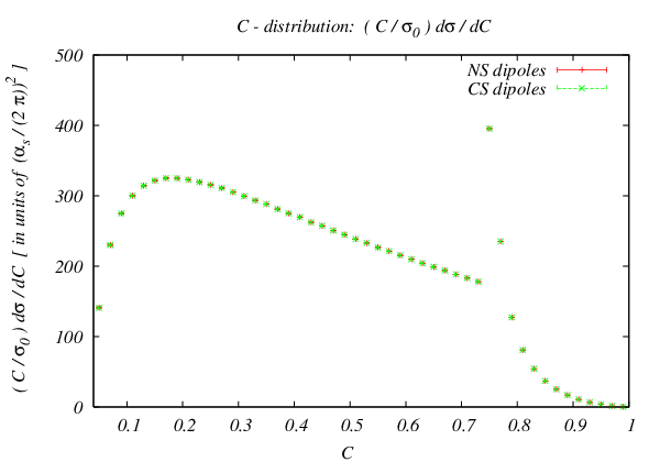
In this section we consider the simplest nontrivial process with more than two partons in the final state: three-jet production in e+​e−e^{+}e^{-} annihilation. The next-to-leading order contributions to this process are well known [57, 81, 82, 83]. We compare the results obtained from the implementation of our scheme and from a private implementation of the Catani Seymour scheme as well as [83]99 9 We thank M. Seymour for help with the original code available from [84].. We find complete agreement for the differential CC parameter [57], with integration errors on the percent level.

The leading order process we consider is given by

e+​e−⟶q⁡(p1)​q¯​(p2)​g​(p3).e^{+}\,e^{-}\,\longrightarrow\,q(p_{1})\,\bar{q}(p_{2})\,g(p_{3}). (69)

At next-to-leading order, two different real-radiation subprocesses contribute:

(A)e+​e−\displaystyle(A)\qquad e^{+}\,e^{-} →\displaystyle\to γ∗​(Q)→q⁡(p^1)​q¯​(p^2)​g​(p^3)​g​(p^4),\displaystyle\gamma^{*}(Q)\,\to\,q(\hat{p}_{1})\,\bar{q}(\hat{p}_{2})\,g(\hat{p}_{3})\,g(\hat{p}_{4}),
(B)e+​e−\displaystyle(B)\qquad e^{+}\,e^{-} →\displaystyle\to γ∗​(Q)→q⁡(p^1)​q¯​(p^2)​q​(p^3)​q¯​(p^4).\displaystyle\gamma^{*}(Q)\,\to\,q(\hat{p}_{1})\,\bar{q}(\hat{p}_{2})\,q(\hat{p}_{3})\,\bar{q}(\hat{p}_{4}). (70)

For a complete next-to-leading order calculation, the virtual corrections need to be added to the leading order contribution. In the following, we use the notation

xi=2​pi⋅Q/Q2,yi​j=si​j/Q2,si​j​k=si​j+si​k+sj​k,x_{i}=2\,p_{i}\cdot Q/Q^{2},\,y_{ij}={s_{ij}}/{Q^{2}},\,s_{ijk}=s_{ij}+s_{ik}+s_{jk},

with si​j=(pi+pj)2s_{ij}\,=\,(p_{i}+p_{j})^{2}. Energy-momentum conservation leads to

∑i,j>iyi​j= 1,∑ixi= 2.\sum_{i,j>i}y_{ij}\,=\,1,\;\sum_{i}\,x_{i}\,=\,2.

We equally follow the notation for matrix elements in Section 3.1:

⟨{pi}|{pi}⟩\displaystyle\left\langle\,\left\{p_{i}\right\}\,\right|\left.\,\left\{p_{i}\right\}\,\right\rangle =\displaystyle= ⟨ℳ3({pi})|ℳ3({pi})⟩≡|ℳ3({pi})|2,\displaystyle\left\langle\,{\cal M}_{3}\left(\left\{p_{i}\right\}\right)\,\right|\left.\,{\cal M}_{3}\left(\left\{p_{i}\right\}\right)\,\right\rangle\,\equiv\,\left|{\cal M}_{3}\left(\left\{p_{i}\right\}\right)\right|^{2},
⟨{p^i}|{p^i}⟩\displaystyle\left\langle\,\left\{\hat{p}_{i}\right\}\,\right|\left.\,\left\{\hat{p}_{i}\right\}\,\right\rangle =\displaystyle= ⟨ℳ4({p^i})|ℳ4({p^i})⟩≡|ℳ4({p^i})|2\displaystyle\left\langle\,{\cal M}_{4}\left(\left\{\hat{p}_{i}\right\}\right)\,\right|\left.\,{\cal M}_{4}\left(\left\{\hat{p}_{i}\right\}\right)\,\right\rangle\,\equiv\,\left|{\cal M}_{4}\left(\left\{\hat{p}_{i}\right\}\right)\right|^{2}

The total next-to-leading order contribution for process (69) is then given by:

σJN​L​O=∫dPS4[|ℳ4({p^i})|2FJ(4)({p^i})−∑ℓ,j⟨q,r,s|𝒟ℓ​j({p^i})|q,r,s⟩FJ(3)(q,r,s)]A\displaystyle\sigma^{NLO}_{J}=\int dPS_{4}\left[\left|{\cal M}_{4}\left(\left\{\hat{p}_{i}\right\}\right)\right|^{2}F_{J}^{(4)}\left(\left\{\hat{p}_{i}\right\}\right)-\sum_{\ell,j}\left\langle q,r,s\right|{\cal D}_{\ell j}\left(\left\{\hat{p}_{i}\right\}\right)\left|q,r,s\right\rangle F_{J}^{(3)}(q,r,s)\right]_{A} (71)
+∫dPS4∑flavours[|ℳ4({p^i})|2FJ(4)({p^i})−∑ℓ,j⟨q,r,s|𝒟ℓ​j({p^i})|q,r,s⟩FJ(3)(q,r,s)]B\displaystyle+\int dPS_{4}\sum_{\textrm{flavours}}\left[\left|{\cal M}_{4}\left(\left\{\hat{p}_{i}\right\}\right)\right|^{2}F_{J}^{(4)}\left(\left\{\hat{p}_{i}\right\}\right)-\sum_{\ell,j}\left\langle q,r,s\right|{\cal D}_{\ell j}\left(\left\{\hat{p}_{i}\right\}\right)\left|q,r,s\right\rangle F_{J}^{(3)}(q,r,s)\right]_{B}
+∫dPS3{|ℳV({pi})|2+12[∑ℓ,jμ2​ε∫dξp⟨1,2,3|𝒟ℓ​j({p^i})|1,2,3⟩]A\displaystyle+\int dPS_{3}\Bigg\{\left|{\cal M}_{V}\left(\left\{p_{i}\right\}\right)\right|^{2}+\frac{1}{2}\left[\sum_{\ell,j}\mu^{2\varepsilon}\int d\xi_{p}\left\langle 1,2,3\right|{\cal D}_{\ell j}\left(\left\{\hat{p}_{i}\right\}\right)\left|1,2,3\right\rangle\right]_{A}\Bigg.
+∑flavours14[∑ℓ,jμ2​ε∫dξp⟨1,2,3|𝒟ℓ​j({p^i})|1,2,3⟩]B}FJ(3)({pi})\displaystyle\Bigg.+\sum_{\textrm{flavours}}\frac{1}{4}\left[\sum_{\ell,j}\mu^{2\varepsilon}\int d\xi_{p}\left\langle 1,2,3\right|{\cal D}_{\ell j}\left(\left\{\hat{p}_{i}\right\}\right)\left|1,2,3\right\rangle\right]_{B}\Bigg\}F_{J}^{(3)}\left(\left\{p_{i}\right\}\right)

where ℓ,j\ell,j sum over all possible pairs in the real emission phase space, p^i\hat{p}_{i} and pip_{i} denote momenta belonging to Born and real emission kinematics, and where q,r,s∈{1,2,3}q,r,s\,\in\,\{1,2,3\} denote the mapped momenta in the real emission subtraction terms for the Born-type matrix elements. The factors 12,14\frac{1}{2},\,\frac{1}{4} in the integrated subtraction terms correspond to the process-dependent symmetry factors in the real emission contributions. In the symbolic notation above, ∫d​P​Sn\int\,dPS_{n} contains all symmetry and flux factors for the respective phase space1010 10 Note that ∫d​P​S3\int\,dPS_{3} and ∫d​P​S4\int\,dPS_{4} are defined slightly differently in [83, 59]..

4.1 Tree level result

In the following, we follow the procedure of [57], i.e. we normalize our observables according to

1σ0​d​σJNLO,\frac{1}{\sigma_{0}}\,d\sigma^{\text{NLO}}_{J},

where σ0\sigma_{0} denotes the total cross section for the process

e+​e−⟶q​q¯e^{+}\,e^{-}\,\longrightarrow\,q\,\bar{q} (72)

given by [57]

σ0=4​π​α23​s​CA​qf2\sigma_{0}\,=\,\frac{4\,\pi\,\alpha^{2}}{3\,s}\,C_{A}\,q_{f}^{2}

for a quark with flavour ff and charge qfq_{f}. We normalize the matrix elements according to

σJ(n)=12​s​S​∫d​Γn​|ℳn|2​FJ(n),\sigma^{(n)}_{J}\,=\,\frac{1}{2\,s}\,S\,\int\,d\Gamma_{n}\,|\mathcal{M}_{n}|^{2}\,F_{J}^{(n)},

where d​Γn=∏i[d4​pi(2​π)4​δ​(pi2−mi2)]​δ(4)​(∑inpin−∑ipi)d\Gamma_{n}\,=\,\prod_{i}\,\left[\frac{d^{4}p_{i}}{(2\pi)^{4}}\,\delta\left(p_{i}^{2}-m_{i}^{2}\right)\right]\,\delta^{(4)}\left(\sum_{\text{in}}p_{\text{in}}-\sum_{i}\,p_{i}\right), ss denotes the center-of-mass energy and

S\displaystyle S =\displaystyle= {1/2!forγ∗→q​q¯​g​g1/2!×1/2!forγ∗→q​q¯​q​q¯\displaystyle\left\{\begin{array}[]{cl}{1}/{2!}&\quad\textrm{for}\quad\gamma^{*}\to q\,\bar{q}\,g\,g\\ &\\ {1}/{2!}\times{1}/{2!}&\quad\textrm{for}\quad\gamma^{*}\to q\,\bar{q}\,q\,\bar{q}\\ \end{array}\right.

is the symmetry factor of the respective process. We obtain the well-known relations between the matrix elements of the processes (72) and (69) [57]:

14​|ℳ3|2=8​π​αss​CF​x12+x22(1−x1)​(1−x2)​14​⟨|ℳ2|2⟩\frac{1}{4}|\mathcal{M}_{3}|^{2}\,=\,\frac{8\,\pi\,\alpha_{s}}{s}\,C_{F}\,\frac{x_{1}^{2}+x_{2}^{2}}{(1-x_{1})\,(1-x_{2})}\,\frac{1}{4}\langle|\mathcal{M}_{2}|^{2}\rangle

where |ℳ2|2|\mathcal{M}_{2}|^{2} has been averaged over the emission angles, as well as

σ3,J=αs2​π​CF​∫d​x1​d​x2​Πi​[Θ⁡(1−xi)​Θ​(xi)]​Θ​(x1+x2−1)​x12+x22(1−x1)​(1−x2)​σ0​FJ(3)​(x1,x2)\sigma_{3,J}\,=\,\frac{\alpha_{s}}{2\,\pi}C_{F}\int dx_{1}dx_{2}\Pi_{i}\left[\Theta(1-x_{i})\Theta(x_{i})\right]\Theta(x_{1}+x_{2}-1)\frac{x_{1}^{2}+x_{2}^{2}}{(1-x_{1})(1-x_{2})}\sigma_{0}F^{(3)}_{J}(x_{1},x_{2})

for jet observables. The gluon-helicity dependent squared matrix element for the leading order process (69) is given by [83]

𝒯μ​ν​(p1,p2,p3)=−1x12+x22​|ℳ3​(p1,p2,p3)|2​Tμ​ν,{\cal T}^{\mu\nu}(p_{1},p_{2},p_{3})=-\frac{1}{x_{1}^{2}+x_{2}^{2}}\,\left|{\cal M}_{3}(p_{1},p_{2},p_{3})\right|^{2}\,T^{\mu\nu}, (74)

where

Tμ​ν\displaystyle T^{\mu\nu} =+2​p1μ​p2νQ2+2​p2μ​p1νQ2−2​1−x11−x2​p1μ​p1νQ2−2​1−x21−x1​p2μ​p2νQ2\displaystyle=+2\,\frac{p_{1}^{\mu}p_{2}^{\nu}}{Q^{2}}+2\,\frac{p_{2}^{\mu}p_{1}^{\nu}}{Q^{2}}-2\,\frac{1-x_{1}}{1-x_{2}}\,\frac{p_{1}^{\mu}p_{1}^{\nu}}{Q^{2}}-2\,\frac{1-x_{2}}{1-x_{1}}\,\frac{p_{2}^{\mu}p_{2}^{\nu}}{Q^{2}}
−1−x1−x2+x221−x2​[p1μ​p3νQ2+p3μ​p1νQ2]−1−x2−x1+x121−x1​[p2μ​p3νQ2+p3μ​p2νQ2]\displaystyle-\frac{1-x_{1}-x_{2}+x_{2}^{2}}{1-x_{2}}\,\left[\frac{p_{1}^{\mu}p_{3}^{\nu}}{Q^{2}}+\frac{p_{3}^{\mu}p_{1}^{\nu}}{Q^{2}}\right]-\frac{1-x_{2}-x_{1}+x_{1}^{2}}{1-x_{1}}\,\left[\frac{p_{2}^{\mu}p_{3}^{\nu}}{Q^{2}}+\frac{p_{3}^{\mu}p_{2}^{\nu}}{Q^{2}}\right]
+(1+12​x12+12​x22−x1−x2)​gμ​ν.\displaystyle+\left(1+\frac{1}{2}\,x_{1}^{2}+\frac{1}{2}\,x_{2}^{2}-x_{1}-x_{2}\right)\,g^{\mu\nu}. (75)

𝒯μ​ν{\cal T}_{\mu\nu} obeys gμ​ν​𝒯μ​ν=−|ℳ3|2g^{\mu\nu}{\cal T}_{\mu\nu}=-|{\cal M}_{3}|^{2}.

The virtual one-loop matrix element

The virtual contribution to the process (69) in the MS¯\overline{\textrm{MS}} renormalization scheme is [57, 59]

|ℳV​(p1,p2,p3)|2=|ℳ3​(p1,p2,p3)|2​αs2​π​(4​π​μ2Q2)ε​1Γ⁡(1−ε)\displaystyle\left|{\cal M}_{V}(p_{1},p_{2},p_{3})\right|^{2}\,=\,\left|{\cal M}_{3}(p_{1},p_{2},p_{3})\right|^{2}\,\frac{\alpha_{s}}{2\pi}\,\left(\frac{4\pi\mu^{2}}{Q^{2}}\right)^{\varepsilon}\,\frac{1}{\Gamma(1-\varepsilon)} (76)
×\displaystyle\times {−1ε2[(2CF−CA)y12−ε+CA(y13−ε+y23−ε)]−1ε(3CF+116CA−23nfTR)\displaystyle\left\{\,-\frac{1}{\varepsilon^{2}}\left[\left(2C_{F}-C_{A}\right)y_{12}^{-\varepsilon}+C_{A}\left(y_{13}^{-\varepsilon}+y_{23}^{-\varepsilon}\right)\right]-\frac{1}{\varepsilon}\,\left(3\,C_{F}+\frac{11}{6}C_{A}-\frac{2}{3}n_{f}\,T_{R}\right)\right.
+π22(2CF+CA)−8CF}+αs2​π[F(y12,y13,y23)+𝒪(ε)],\displaystyle+\left.\frac{\pi^{2}}{2}\,(2\,C_{F}+C_{A})-8\,C_{F}\right\}+\frac{\alpha_{s}}{2\pi}\,\left[F(y_{12},y_{13},y_{23})+{\cal O}(\varepsilon)\right],

where F⁡(y12,y13,y23)F(y_{12},y_{13},y_{23}) is defined in Eqn. (2.21) of [57].

4.2 Subtraction terms

In general, the subtraction terms are given by Eqn. (67) as

𝒟ℓ​j≡𝒟fℓ​f^ℓ​f^j​(p^ℓ,p^j)=𝒟fℓ​f^ℓ​f^jcoll​(p^ℓ,p^j)+δf^j,g​∑k≠(ℓ,j)𝒟if​(p^ℓ,p^j,p^k),\mathcal{D}_{\ell j}\,\equiv\,\mathcal{D}_{f_{\ell}\hat{f}_{\ell}\hat{f}_{j}}(\hat{p}_{\ell},\hat{p}_{j})\,=\,\mathcal{D}^{\text{coll}}_{f_{\ell}\hat{f}_{\ell}\hat{f}_{j}}(\hat{p}_{\ell},\hat{p}_{j})\,+\,\delta_{\hat{f}_{j},g}\sum_{k\,\neq\,(\ell,j)}\mathcal{D}^{\text{if}}(\hat{p}_{\ell},\hat{p}_{j},\hat{p}_{k}),

where the first part is the collinear subtraction term, and the second the sum over all interference terms. For the processes considered here, the interference terms only contribute to (A)(A), while (B)(B) only contains collinear divergences. In the following sections we will construct the subtraction terms for subprocesses (A)(A) and (B)(B), respectively.

4.2.1 Momentum mapping

For all subtraction terms, the mm-parton phase space momenta are mapped as described in section 3.2.2; i.e. , for a splitting

pℓ→p^ℓ+p^j,p_{\ell}\,\rightarrow\,\hat{p}_{\ell}+\hat{p}_{j},

we have

pℓ\displaystyle p_{\ell} =\displaystyle= 1λ​Pℓ−1−λ+y2​λ​aℓ​Q,\displaystyle\frac{1}{\lambda}\,P_{\ell}-\frac{1-\lambda+y}{2\,\lambda\,a_{\ell}}\,Q,
pk\displaystyle p_{k} =\displaystyle= Λ(K,K^)p^k,[k≠(ℓ,j)]\displaystyle\Lambda(K,\hat{K})\,\hat{p}_{k},\;\;\;[k\,\neq\,(\ell,j)]

where Λ\Lambda is defined according to Eqn. (33), and where

K^=Q−Pℓ,K=Q−pℓ.\hat{K}\,=\,Q-P_{\ell},\;K\,=\,Q-p_{\ell}.

4.2.2 The subprocess: 𝜸∗→𝒒⁡(𝒑^𝟏)​𝒒¯​(𝒑^𝟐)​𝒈​(𝒑^𝟑)​𝒈​(𝒑^𝟒)\boldsymbol{\gamma^{*}\,\to\,q(\hat{p}_{1})\,\bar{q}(\hat{p}_{2})\,g(\hat{p}_{3})\,g(\hat{p}_{4})}

For this process, g​g​g,q​q​gggg,\,qqg\, collinear as well as interference terms need to be taken into account; these are given by Eqns. (58), (46), and (61) respectively. We have for the collinear subtraction terms

𝒟q​q​g;ℓ​jcoll\displaystyle\mathcal{D}^{\text{coll}}_{qqg;\ell j} =\displaystyle= 4​π​αsy⁡(pℓ⋅Q)​CF​{(λ−1+y)2+4​y4​λ​Feik+12​z​[1+y+λ]},\displaystyle\frac{4\,\pi\,\alpha_{s}}{y\,(p_{\ell}\cdot Q)}\,C_{F}\,\left\{\frac{(\lambda-1+y)^{2}+4\,y}{4\,\lambda}\,F_{\text{eik}}\,+\,\frac{1}{2}\,z\,\left[1+y+\lambda\right]\right\},
⟨ν|𝒟g​g​g;ℓ​jcoll|ν′⟩​𝒯ν​ν′\displaystyle\langle\nu|\mathcal{D}^{\text{coll}}_{ggg;\ell j}|\nu^{\prime}\rangle\,\mathcal{T}^{\nu\nu^{\prime}} =\displaystyle= −2παsCA1(p^ℓ⋅p^j)2[2−Δ(2−Δ)]1x12+x22|ℳ3(p1,p2,p3)|2×\displaystyle-2\,\pi\,\alpha_{s}\,C_{A}\,\frac{1}{(\hat{p}_{\ell}\cdot\hat{p}_{j})^{2}}\,\left[2-\Delta(2-\Delta)\right]\,\frac{1}{x_{1}^{2}+x_{2}^{2}}|\mathcal{M}_{3}(p_{1},p_{2},p_{3})|^{2}\,\times
{[2Q2(2(k⟂⋅p1)(k⟂⋅p2)−1−x11−x2(k⟂⋅p1)2−1−x21−x1(k⟂⋅p2)2)\displaystyle\Bigg\{\left[\frac{2}{Q^{2}}\left(2(k_{\perp}\cdot p_{1})(k_{\perp}\cdot p_{2})-\frac{1-x_{1}}{1-x_{2}}(k_{\perp}\cdot p_{1})^{2}-\frac{1-x_{2}}{1-x_{1}}(k_{\perp}\cdot p_{2})^{2}\right)\right.
+k⟂2(1+x122+x222−x1−x2)]},\displaystyle\left.\,+\,k_{\perp}^{2}\,\left(1+\frac{x_{1}^{2}}{2}+\frac{x_{2}^{2}}{2}-x_{1}-x_{2}\right)\right]\Bigg\},

with k⟂k_{\perp} and Δ\Delta given by Eqns. (49) and (54). In total, we need to consider the following combinations:

𝒟q​q​g;13coll,𝒟q​q​g;14coll,𝒟q​q​g;23coll,𝒟q​q​g;24coll,𝒟g​g​g;34coll,𝒟g​g​g;43coll;\mathcal{D}^{\text{coll}}_{qqg;13},\,\mathcal{D}^{\text{coll}}_{qqg;14},\,\mathcal{D}^{\text{coll}}_{qqg;23},\,\mathcal{D}^{\text{coll}}_{qqg;24},\,\mathcal{D}^{\text{coll}}_{ggg;34},\,\mathcal{D}^{\text{coll}}_{ggg;43};

note especially that both combinations (3,4),(4,3)(3,4),(4,3) need to be taken into account in the contributions from g​g​gggg splittings.

The interference terms are given by

𝒟ℓ,j;kif=Δ​Wℓ​j​(k)= 4​π​αs​Cℓ​k​2​p^ℓ⋅p^k​p^ℓ⋅Q^p^ℓ⋅p^j​(p^j⋅p^k​p^ℓ⋅Q^+p^ℓ⋅p^j​p^k⋅Q^),{\cal D}^{\text{if}}_{\ell,j;k}\,=\Delta W_{\ell j}(k)\,=\,4\,\pi\,\alpha_{s}\,C_{\ell k}\,\frac{2\,\hat{p}_{\ell}\cdot\hat{p}_{k}\,\hat{p}_{\ell}\cdot\hat{Q}}{\hat{p}_{\ell}\cdot\hat{p}_{j}\,\left(\hat{p}_{j}\cdot\hat{p}_{k}\,\hat{p}_{\ell}\cdot\hat{Q}+\hat{p}_{\ell}\cdot\hat{p}_{j}\,\hat{p}_{k}\cdot\hat{Q}\right)}, (77)

where we have the following contributions:

𝒟1,3;2if,𝒟1,3;4if,𝒟1,4;2if,𝒟1,4;3if,𝒟2,3;1if,𝒟2,3;4if,𝒟2,4;1if,𝒟2,4;3if,𝒟3,4;1if,𝒟3,4;2if,𝒟4,3;1if,𝒟4,3;2if.{\cal D}^{\text{if}}_{1,3;2},\,{\cal D}^{\text{if}}_{1,3;4},\,{\cal D}^{\text{if}}_{1,4;2},\,{\cal D}^{\text{if}}_{1,4;3},{\cal D}^{\text{if}}_{2,3;1},\,{\cal D}^{\text{if}}_{2,3;4},\,{\cal D}^{\text{if}}_{2,4;1},\,{\cal D}^{\text{if}}_{2,4;3},{\cal D}^{\text{if}}_{3,4;1},\,{\cal D}^{\text{if}}_{3,4;2},\,{\cal D}^{\text{if}}_{4,3;1},\,{\cal D}^{\text{if}}_{4,3;2}.

We want to emphasize again that there is only one mapping required for each (ℓ,j)(\ell,j) pairing, i.e. we only have 5 independent mappings for the 12 subtraction terms listed above1111 11 The Catani Seymour prescription [59] requires 10 different mappings for this contribution.. The subtracted cross section is then given by

σR−A=∫4\displaystyle\sigma^{R-A}\,=\,\int_{4}\, [d​σR−d​σA]\displaystyle\left[d\sigma^{R}\,-\,d\sigma^{A}\right]
=∫d​P​S4\displaystyle=\,\int\,dPS_{4}\, {|ℳ4(p^1,p^2,p^3,p^4)|2F4(p^1,p^2,p^3,p^4)\displaystyle\left\{\,\frac{}{}\left|{\cal M}_{4}(\hat{p}_{1},\hat{p}_{2},\hat{p}_{3},\hat{p}_{4})\right|^{2}\,F_{4}(\hat{p}_{1},\hat{p}_{2},\hat{p}_{3},\hat{p}_{4})\right.
−⟨ 1,2,3|𝒟13+𝒟14+𝒟23+𝒟24+𝒟34+𝒟43| 1,2,3⟩F3(p1,p2,p3)}\displaystyle\left.-\langle\,1,2,3\,|\,\mathcal{D}_{13}+\mathcal{D}_{14}+\mathcal{D}_{23}+\mathcal{D}_{24}+\mathcal{D}_{34}+\mathcal{D}_{43}\,|\,1,2,3\,\rangle F_{3}(p_{1},p_{2},p_{3})\,\frac{}{}\right\}

with the spin-averaged matrix element

14​|ℳ4​(p^1,p^2,p^3,p^4)|2\displaystyle\frac{1}{4}\left|{\cal M}_{4}(\hat{p}_{1},\hat{p}_{2},\hat{p}_{3},\hat{p}_{4})\right|^{2} =σ0(αs2​π)2CF 4(4π)5×\displaystyle=\sigma_{0}\,\left(\frac{\alpha_{s}}{2\,\pi}\right)^{2}\,C_{F}\,4\,\left(4\,\pi\right)^{5}\times
{(A+B+C)+(1↔2)+(3↔4)+(1↔2,3↔4)}\displaystyle\,\left\{(A+B+C)+(1\leftrightarrow 2)+(3\leftrightarrow 4)+(1\leftrightarrow 2,3\leftrightarrow 4)\right\} (79)

The quantities A,B,CA,B,C are given in Appendix B of [57].

4.2.3 The subprocess: 𝜸∗→𝒒⁡(𝒑^𝟏)​𝒒¯​(𝒑^𝟐)​𝒒​(𝒑^𝟑)​𝒒¯​(𝒑^𝟒)\boldsymbol{\gamma^{*}\,\to\,q(\hat{p}_{1})\,\bar{q}(\hat{p}_{2})\,q(\hat{p}_{3})\,\bar{q}(\hat{p}_{4})}

This process does not contain any soft/ interference singularities, and all subtraction terms are given by Eqn. (51). We need to keep track of the mother parton’s helicity in the subtraction term and obtain

⟨ν|𝒟g​q​q;ℓ​j|ν′⟩𝒯ν​ν′= 4παsTR1p^ℓ⋅p^j|ℳ3(p1,p2,p3)|2×\displaystyle\langle\nu|{\cal D}_{gqq;\ell j}|\nu^{\prime}\rangle\,\mathcal{T}^{\nu\,\nu^{\prime}}\,=\,4\,\pi\,\alpha_{s}\,T_{R}\,\frac{1}{\hat{p}_{\ell}\cdot\hat{p}_{j}}\,|\mathcal{M}_{3}(p_{1},p_{2},p_{3})|^{2}\,\times
{1+2x12+x221p^ℓ⋅p^j[2Q2(2(k⟂⋅p1)(k⟂⋅p2)−1−x11−x2(k⟂⋅p1)2−1−x21−x1(k⟂⋅p2)2)\displaystyle\Bigg\{1\,+\,\frac{2}{x_{1}^{2}+x_{2}^{2}}\,\frac{1}{\hat{p}_{\ell}\cdot\hat{p}_{j}}\,\left[\frac{2}{Q^{2}}\,\left(2\,(k_{\perp}\cdot\,p_{1})\,(k_{\perp}\cdot p_{2})-\frac{1-x_{1}}{1-x_{2}}(k_{\perp}\cdot\,p_{1})^{2}-\frac{1-x_{2}}{1-x_{1}}(k_{\perp}\cdot\,p_{2})^{2}\right)\right.
+k⟂2(1+x122+x222−x1−x2)]},\displaystyle\left.\,+\,k_{\perp}^{2}\,\left(1+\frac{x_{1}^{2}}{2}+\frac{x_{2}^{2}}{2}-x_{1}-x_{2}\right)\right]\Bigg\},

with k⟂k_{\perp} and k⟂2k_{\perp}^{2} given by Eqns. (49) and (55) respectively.

We have to consider the following combinations

𝒟g​q​q;12,𝒟g​q​q;14,𝒟g​q​q;32,𝒟g​q​q;34\displaystyle{\cal D}_{gqq;12},\,{\cal D}_{gqq;14},\,{\cal D}_{gqq;32},\,{\cal D}_{gqq;34} (80)

and get

σR−A=∫4\displaystyle\sigma^{R-A}\,=\,\int_{4}\, [d​σR−d​σA]\displaystyle\left[d\sigma^{R}\,-\,d\sigma^{A}\right]
=∫d​P​S4\displaystyle=\,\int\,dPS_{4}\, {|ℳ4(p^1,p^2,p^3,p^4)|2F4(p^1,p^2,p^3,p^4)\displaystyle\left\{\,\frac{}{}\left|{\cal M}_{4}(\hat{p}_{1},\hat{p}_{2},\hat{p}_{3},\hat{p}_{4})\right|^{2}\,F_{4}(\hat{p}_{1},\hat{p}_{2},\hat{p}_{3},\hat{p}_{4})\right.
−⟨ 1,2,3|𝒟13+𝒟14+𝒟32+𝒟34| 1,2,3⟩F3(p1,p2,p3)}\displaystyle\left.-\langle\,1,2,3\,|\,\mathcal{D}_{13}+\mathcal{D}_{14}+\mathcal{D}_{32}+\mathcal{D}_{34}|\,1,2,3\,\rangle F_{3}(p_{1},p_{2},p_{3})\,\frac{}{}\right\}

with the spin-averaged matrix element given by

14​|ℳ4​(p^1,p^2,p^3,p^4)|2\displaystyle\frac{1}{4}\left|{\cal M}_{4}(\hat{p}_{1},\hat{p}_{2},\hat{p}_{3},\hat{p}_{4})\right|^{2} =σ0(αs2​π)2CF 4(4π)5×\displaystyle=\sigma_{0}\,\left(\frac{\alpha_{s}}{2\,\pi}\right)^{2}\,C_{F}\,4\,\left(4\,\pi\right)^{5}\,\times
{(D+E)+(1↔2)+(3↔4)+(1↔2,3↔4)}\displaystyle\left\{(D+E)+(1\leftrightarrow 2)+(3\leftrightarrow 4)+(1\leftrightarrow 2,3\leftrightarrow 4)\right\} (82)

The quantities DD and EE are given in Appendix B of [57].

4.3 Integrated subtraction terms

4.3.1 Collinear integrals

The collinear integrals involve the g​q​q¯gq\bar{q}, q​q​g/q¯​q¯​gqqg/{\bar{q}\bar{q}g} and g​g​gggg splittings:

Icoll=Icoll​(g​q​q¯)+Icoll​(q​q​g)+Icoll​(g​g​g).I_{\textrm{coll}}\,=\,I_{\textrm{coll}}(gq\bar{q})\,+\,I_{\textrm{coll}}(qqg)\,+\,I_{\textrm{coll}}(ggg). (83)

After summing over all contributions, we obtain from Eqns. (3.3), (47) and (3.3)

⟨1,2,3​|Icoll​(g​q​q¯)|​1,2,3⟩B=\displaystyle\langle 1,2,3\left|\,I_{\textrm{coll}}(gq\bar{q})\,\right|1,2,3\rangle_{B}\,=\,
|ℳ3(p1,p2,p3)|2αs2​πTR(4​π​μ2Q2)ε1Γ⁡(1−ε)nf×\displaystyle\left|{\cal M}_{3}(p_{1},p_{2},p_{3})\right|^{2}\frac{\alpha_{s}}{2\,\pi}\,T_{R}\,\left(\frac{4\,\pi\,\mu^{2}}{Q^{2}}\right)^{\varepsilon}\,\frac{1}{\Gamma(1-\varepsilon)}\,n_{f}\,\times
[−23​ε−169+23​[(a3−1)​ln⁡(a3−1)−(a3+1)​ln⁡a3]],\displaystyle\left[-\frac{2}{3\,\varepsilon}\,-\,\frac{16}{9}\,+\,\frac{2}{3}\,\left[(a_{3}-1)\,\ln(a_{3}-1)-(a_{3}+1)\,\ln\,a_{3}\right]\right],
⟨1,2,3​|Icoll​(q​q​g)|​1,2,3⟩A=\displaystyle\langle 1,2,3\left|\,I_{\textrm{coll}}(qqg)\,\right|1,2,3\rangle_{A}\,=\,
|ℳ3(p1,p2,p3)|2αs2​πCF(4​π​μ2Q2)ε1Γ⁡(1−ε)×\displaystyle\left|{\cal M}_{3}(p_{1},p_{2},p_{3})\right|^{2}\frac{\alpha_{s}}{2\,\pi}\,C_{F}\,\left(\frac{4\,\pi\,\mu^{2}}{Q^{2}}\right)^{\varepsilon}\,\frac{1}{\Gamma(1-\varepsilon)}\,\times\,
12∑ℓ=1,2{−1ε+ 4I3(aℓ)−lnaℓ+12[(9−7aℓ)(aℓ−1)ln(aℓ−1)+aℓ(7aℓ−16)log(aℓ)\displaystyle\frac{1}{2}\sum_{\ell=1,2}\Bigg\{-\frac{1}{\varepsilon}+\,4\,I_{3}(a_{\ell})\,-\,\ln\,a_{\ell}+\frac{1}{2}\left[(9-7a_{\ell})(a_{\ell}-1)\ln(a_{\ell}-1)+a_{\ell}(7a_{\ell}-16)\log(a_{\ell})\right.
−7log(ymax(aℓ))−aℓ(2ymax(aℓ)+7)−7ymax(aℓ)−4]}\displaystyle\left.-7\log(y_{\text{max}}(a_{\ell}))-a_{\ell}(2y_{\text{max}}(a_{\ell})+7)-7y_{\text{max}}(a_{\ell})-4\right]\Bigg\}
⟨1,2,3|Icoll(ggg)|1,2,3⟩A⟩=\displaystyle\langle 1,2,3\left|\,I_{\textrm{coll}}(ggg)\,\right|1,2,3\rangle_{A}\,\rangle\,=\, (84)
|ℳ3(p1,p2,p3)|2αs2​πCA(4​π​μ2Q2)ε1Γ⁡(1−ε)×\displaystyle\left|{\cal M}_{3}(p_{1},p_{2},p_{3})\right|^{2}\frac{\alpha_{s}}{2\,\pi}\,C_{A}\,\left(\frac{4\,\pi\,\mu^{2}}{Q^{2}}\right)^{\varepsilon}\,\frac{1}{\Gamma(1-\varepsilon)}\,\times\,
{−16​ε−49+16​[(a3−1)​ln⁡(a3−1)−(a3+1)​ln⁡a3]+Ifin​(a3)},\displaystyle\left\{-\frac{1}{6\,\varepsilon}\,-\,\frac{4}{9}\,+\,\frac{1}{6}\,\left[(a_{3}-1)\,\ln(a_{3}-1)\,-\,(a_{3}+1)\ln\,a_{3}\right]\,+\,I_{\text{fin}}(a_{3})\right\},

where all symmetry factors have already been taken into account. Here, IfinI_{\text{fin}} and I3I_{3} are given by Eqns. (60) and (48) respectively and need to be evaluated numerically.

4.3.2 Soft integrals

For a specific emitter/ spectator pair (pℓ,pk)(p_{\ell},p_{k}), we obtain from Eqn. (3.3.3)

Isoft,ℓ​k=4​π​αs2​Cℓ​k​μ2​ε​∫d​ξp​Δ​Wℓ​k=\displaystyle I_{\textrm{soft},\ell k}\,=\,\frac{4\,\pi\,\alpha_{s}}{2}\,C_{\ell k}\,\mu^{2\varepsilon}\int d\xi_{p}\,\Delta W_{\ell k}=
αs2​πCℓ​k(4​π​μ2Q2)ε1Γ⁡(1−ε)×{12​ε2+1ε[1+12ln[(a~0(ℓ​k)+aℓ)aℓ]]−π26+ 3\displaystyle\frac{\alpha_{s}}{2\,\pi}\,C_{\ell k}\,\left(\frac{4\pi\mu^{2}}{Q^{2}}\right)^{\varepsilon}\frac{1}{\Gamma(1-\varepsilon)}\times\Bigg\{\frac{1}{2\,\varepsilon^{2}}\,+\,\frac{1}{\varepsilon}\,\left[1\,+\,\frac{1}{2}\,\ln\left[(\tilde{a}^{(\ell k)}_{0}+a_{\ell})\,a_{\ell}\right]\right]\,-\,\frac{\pi^{2}}{6}\,+\,3
+1π​[I~fin(b)​(a~0(ℓ​k)aℓ)+Ifin(d)​(a~(ℓ​k),aℓ)+Ifin(e)​(aℓ)]+14​ln2​[(a~0(ℓ​k)+aℓ)​aℓ]\displaystyle\,+\,\frac{1}{\pi}\left[\tilde{I}^{(b)}_{\text{fin}}\left(\frac{\tilde{a}^{(\ell k)}_{0}}{a_{\ell}}\right)\,+\,I^{(d)}_{\text{fin}}(\tilde{a}^{(\ell k)},a_{\ell})\,+\,I^{(e)}_{\text{fin}}(a_{\ell})\right]+\,\frac{1}{4}\,\ln^{2}\left[(\tilde{a}^{(\ell k)}_{0}+a_{\ell})\,a_{\ell}\right]
−ln 2ln(a~0(ℓ​k)+aℓaℓ)+2lnaℓ},\displaystyle\,-\ln\,2\,\ln\left(\frac{\tilde{a}^{(\ell k)}_{0}+a_{\ell}}{a_{\ell}}\right)+2\,\ln\,a_{\ell}\Bigg\}, (85)

where

I~fin(b)​(b)≡Ifin(b)​(b)−π⁡[ln⁡ 2​ln⁡(1+b)+14​ln2⁡(1+b)].\tilde{I}_{\text{fin}}^{(b)}(b)\,\equiv\,I_{\text{fin}}^{(b)}(b)-\pi\left[\ln\,2\,\ln(1+b)\,+\,\frac{1}{4}\,\ln^{2}(1+b)\right].

The additional factor 12\frac{1}{2} in the integrated subtraction terms stems from Eqn. (68) and accounts for the different symmetry factors and combinatorics of process (A). Soft interference terms only appear for this process, where the following emitter/ spectator pairs need to be taken into account

2​[(1,2)+(1,3)+(2,1)+(2,3)+(3,1)+(3,2)];2\,\left[(1,2)+(1,3)+(2,1)+(2,3)+(3,1)+(3,2)\right]; (86)

the factor 22 arises as e.g. (p^ℓ,p^j,p^k)=[(p^1​p^3,p^2),(p^1​p^4,p^2)](\hat{p}_{\ell},\hat{p}_{j},\hat{p}_{k})\,=\,\left[(\hat{p}_{1}\,\hat{p}_{3},\,\hat{p}_{2}),(\hat{p}_{1}\,\hat{p}_{4},\,\hat{p}_{2})\right] are mapped to the same Born-type kinematics (pℓ,pk)=(p1,p2)(p_{\ell},p_{k})\,=\,(p_{1},p_{2}), and similar relations hold for the other contributions.

4.3.3 Finite parts

Combining the one-loop matrix element Eqn. (76) with the integrated subtraction terms, all poles in ε\varepsilon cancel. The leftover finite parts are

<1,2,3|Icoll|1,2,3>finite=|ℳ3(p1,p2,p3)|2αs2​π×\displaystyle<1,2,3\left|\,I_{\text{coll}}\,\right|1,2,3>_{\textrm{finite}}\,=\,\,\left|{\cal M}_{3}(p_{1},p_{2},p_{3})\right|^{2}\,\frac{\alpha_{s}}{2\,\pi}\,\,\times
{(4nfTR+CA)[−49+16[(a3−1)ln(a3−1)−(a3+1)lna3]]+CAIfin(a3)\displaystyle\Bigg\{\left(4\,n_{f}\,T_{R}+C_{A}\right)\,\left[-\frac{4}{9}\,+\,\frac{1}{6}\,\left[(a_{3}-1)\,\ln(a_{3}-1)-(a_{3}+1)\,\ln\,a_{3}\right]\right]+C_{A}\,I_{\text{fin}}(a_{3})
+CF2∑ℓ=1,2[4I3(aℓ)−lnaℓ+12[(9−7aℓ)(aℓ−1)ln(aℓ−1)+aℓ(7aℓ−16)log(aℓ)\displaystyle+\,\frac{C_{F}}{2}\sum_{\ell=1,2}\Bigg[4\,I_{3}(a_{\ell})\,-\,\ln\,a_{\ell}+\frac{1}{2}\left[(9-7a_{\ell})(a_{\ell}-1)\ln(a_{\ell}-1)+a_{\ell}(7a_{\ell}-16)\log(a_{\ell})\right.
−7log(ymax(aℓ))−aℓ(2ymax(aℓ)+7)−7ymax(aℓ)−4]]}\displaystyle\hskip 71.13188pt\left.-7\log(y_{\text{max}}(a_{\ell}))-a_{\ell}(2y_{\text{max}}(a_{\ell})+7)-7y_{\text{max}}(a_{\ell})-4\right]\Bigg]\Bigg\} (87)

and

<1,2,3|Isoft|1,2,3>finite=|ℳ3(p1,p2,p3)|2αs2​π×\displaystyle<1,2,3\left|\,I_{\text{soft}}\,\right|1,2,3>_{\textrm{finite}}\,=\,\,\left|{\cal M}_{3}(p_{1},p_{2},p_{3})\right|^{2}\,\frac{\alpha_{s}}{2\,\pi}\,\,\times
{(2CF+CA)[−π23+6]+2∑ℓ=1,2,3Cℓ2[1πIfin(e)(aℓ)+2lnaℓ]\displaystyle\Bigg\{\left(2\,C_{F}+C_{A}\right)\,\left[-\frac{\pi^{2}}{3}+6\right]+2\,\sum_{\ell=1,2,3}\,C_{\ell}^{2}\,\left[\frac{1}{\pi}I^{(e)}_{\text{fin}}(a_{\ell})+2\,\ln\,a_{\ell}\right]
−2​(CA−2​CF)​[1π​I~fin(b)​(a~0(1,2)a1)−ln⁡ 2​ln⁡(a~0(1,2)a1+1)]\displaystyle-2\,\left(C_{A}-2\,C_{F}\right)\,\left[\frac{1}{\pi}\,\tilde{I}^{(b)}_{\text{fin}}\left(\frac{\tilde{a}_{0}^{(1,2)}}{a_{1}}\right)\,-\,\ln\,2\,\ln\left(\frac{\tilde{a}_{0}^{(1,2)}}{a_{1}}+1\right)\right]
+2CA∑ℓ=1,2[1πI~fin(b)(a~0(ℓ,3)aℓ)−ln 2ln(a~0(ℓ,3)aℓ+1)]\displaystyle+2\,C_{A}\,\sum_{\ell=1,2}\left[\frac{1}{\pi}\,\tilde{I}^{(b)}_{\text{fin}}\left(\frac{\tilde{a}_{0}^{(\ell,3)}}{a_{\ell}}\right)\,-\,\ln\,2\,\ln\left(\frac{\tilde{a}_{0}^{(\ell,3)}}{a_{\ell}}+1\right)\right]
+∑(ℓ,k)Cℓ​k[2πIfin(d)(a~(ℓ,k),aℓ)+12ln2[(a~0(ℓ,k)+aℓ)aℓ]]},\displaystyle+\sum_{(\ell,k)}C_{\ell k}\,\left[\frac{2}{\pi}I^{(d)}_{\text{fin}}\,\left(\tilde{a}^{(\ell,k)},a_{\ell}\right)+\frac{1}{2}\,\ln^{2}\left[\left(\tilde{a}_{0}^{(\ell,k)}+a_{\ell}\right)a_{\ell}\right]\right]\Bigg\}, (88)

where the sum in the last line goes over all possible combinations as given in Eqn. (86) (the factor 2 is already accounted for), and where we made use of several symmetries1212 12 One useful relation is e.g.  a~0(m,n)an=a~0(n,m)am.\frac{\tilde{a}_{0}^{(m,n)}}{a_{n}}\,=\,\frac{\tilde{a}_{0}^{(n,m)}}{a_{m}}. . Further simplifications for the interference term finally render

<1,2,3|Isoft|1,2,3>finite=|ℳ3(p1,p2,p3)|2αs2​π×\displaystyle<1,2,3\left|\,I_{\text{soft}}\,\right|1,2,3>_{\textrm{finite}}\,=\,\,\left|{\cal M}_{3}(p_{1},p_{2},p_{3})\right|^{2}\,\frac{\alpha_{s}}{2\,\pi}\,\,\times
{(2CF+CA)[−π23+6]+2∑ℓ=1,2,3Cℓ2[1πIfin(e)(aℓ)+2lnaℓ]\displaystyle\Bigg\{\left(2\,C_{F}+C_{A}\right)\,\left[-\frac{\pi^{2}}{3}+6\right]+2\,\sum_{\ell=1,2,3}\,C_{\ell}^{2}\,\left[\frac{1}{\pi}I^{(e)}_{\text{fin}}(a_{\ell})+2\,\ln\,a_{\ell}\right]
+12​CA​{2​[ln⁡a1​ln​a2−ln⁡a3​ln⁡(a1​a2a3)]+ln2⁡y13+ln2⁡y23−ln2⁡y12}\displaystyle+\frac{1}{2}C_{A}\,\left\{2\,\left[\ln\,a_{1}\,\ln\,a_{2}-\ln\,a_{3}\,\ln\left(\frac{a_{1}\,a_{2}}{a_{3}}\right)\right]+\,\ln^{2}\,y_{13}\,+\ln^{2}\,y_{23}\,-\ln^{2}\,y_{12}\right\}
+CF​[ln2⁡(a1a2)+ln2⁡y12]+2​ln​ 2​[2​CF​ln⁡(y12​a1​a2)−CA​ln​y12y13​y23​a32]\displaystyle+\,C_{F}\,\left[\ln^{2}\left(\frac{a_{1}}{a_{2}}\right)\,+\,\ln^{2}y_{12}\right]\,+2\,\ln\,2\,\left[2\,C_{F}\,\ln\,\left(y_{12}\,a_{1}\,a_{2}\right)-C_{A}\,\ln\frac{y_{12}}{y_{13}y_{23}a_{3}^{2}}\right]
+2π[CA∑ℓ=1,2I~fin(b)(1yℓ​3​aℓ​a3)−(CA−2CF)I~fin(b)(1y12​a1​a2)+∑(ℓ,k)Cℓ​kIfin(d)(a~(ℓ,k),aℓ)]}\displaystyle+\frac{2}{\pi}\left[C_{A}\sum_{\ell=1,2}\tilde{I}^{(b)}_{\text{fin}}\left(\frac{1}{y_{\ell 3}a_{\ell}a_{3}}\right)-\left(C_{A}-2C_{F}\right)\tilde{I}^{(b)}_{\text{fin}}\left(\frac{1}{y_{12}a_{1}a_{2}}\right)+\sum_{(\ell,k)}C_{\ell k}\,I^{(d)}_{\text{fin}}\left(\tilde{a}^{(\ell,k)},a_{\ell}\right)\right]\Bigg\} (89)

4.3.4 Final expressions

The finite parts of one-loop matrix element are given by

|ℳV(p1,p2,p3)|finite2=|ℳ3(p1,p2,p3)|2αs2​π×\displaystyle\left|{\cal M}_{V}(p_{1},p_{2},p_{3})\right|^{2}_{\textrm{finite}}\,=\,\left|{\cal M}_{3}(p_{1},p_{2},p_{3})\right|^{2}\,\frac{\alpha_{s}}{2\pi}\,\times
{​12​[​(CA−2​CF)​ln2​y12−CA​(ln2⁡y13+ln2⁡y23)​]+π22​(2​CF+CA)−8​CF​}\displaystyle\left\{\frac{}{}\frac{1}{2}\left[\frac{}{}\left(C_{A}-2\,C_{F}\right)\ln^{2}y_{12}-C_{A}\left(\ln^{2}y_{13}+\ln^{2}y_{23}\right)\frac{}{}\right]+\frac{\pi^{2}}{2}\,(2\,C_{F}+C_{A})-8\,C_{F}\frac{}{}\right\}
+αs2​π​[​F​(y12,y13,y23)+𝒪⁡(ε)​]\displaystyle+\frac{\alpha_{s}}{2\pi}\,\left[\frac{}{}F(y_{12},y_{13},y_{23})+{\cal O}(\varepsilon)\frac{}{}\right] (90)

If we combine the one-loop matrix element with the integrated subtraction terms, poles in ε\varepsilon exactly cancel, leading to finite results:

σV+A=∫3[d​σV+∫1d​σA]\displaystyle\sigma^{V+A}=\int_{3}\,\left[d\sigma^{V}+\int_{1}d\sigma^{A}\right]
=∫d​P​S3​{⟨1,2,3​|Isoft|​1,2,3⟩+⟨1,2,3​|Icoll|​1,2,3⟩+|ℳV​(p1,p2,p3)|2}​F3​(p1,p2,p3)\displaystyle=\int dPS_{3}\Bigg\{\langle 1,2,3\left|I_{\textrm{soft}}\right|1,2,3\rangle+\langle 1,2,3\left|\,I_{\textrm{coll}}\right|1,2,3\rangle+\left|{\cal M}_{V}(p_{1},p_{2},p_{3})\right|^{2}\Bigg\}F_{3}(p_{1},p_{2},p_{3})
=∫d​P​S3​{⟨1,2,3​|Isoft|​1,2,3⟩fin+⟨1,2,3​|Icoll|​1,2,3⟩fin+|ℳV​(p1,p2,p3)|fin2}​F3​(p1,p2,p3)\displaystyle=\int dPS_{3}\Bigg\{\langle 1,2,3\left|I_{\textrm{soft}}\right|1,2,3\rangle_{\textrm{fin}}+\langle 1,2,3\left|I_{\textrm{coll}}\right|1,2,3\rangle_{\textrm{fin}}+\left|{\cal M}_{V}(p_{1},p_{2},p_{3})\right|^{2}_{\textrm{fin}}\Bigg\}F_{3}(p_{1},p_{2},p_{3})

where

⟨1,2,3​|Isoft|​1,2,3⟩fin+⟨1,2,3​|Icoll|​1,2,3⟩fin+|ℳV​(p1,p2,p3)|fin2\displaystyle\langle 1,2,3\left|I_{\textrm{soft}}\right|1,2,3\rangle_{\textrm{fin}}+\langle 1,2,3\left|I_{\textrm{coll}}\right|1,2,3\rangle_{\textrm{fin}}+\left|{\cal M}_{V}(p_{1},p_{2},p_{3})\right|^{2}_{\textrm{fin}}
=|ℳ3(p1,p2,p3)|2αs2​π×\displaystyle\,=\left|{\cal M}_{3}(p_{1},p_{2},p_{3})\right|^{2}\,\frac{\alpha_{s}}{2\pi}\,\times
{(2CF+CA)π26+2CF+509CA−169nfTR+72CFln(a1a2)\displaystyle\Bigg\{(2\,C_{F}+C_{A})\frac{\pi^{2}}{6}+2\,C_{F}\,+\,\frac{50}{9}\,C_{A}\,-\,\frac{16}{9}\,n_{f}\,T_{R}\,+\frac{7}{2}\,C_{F}\,\ln\left(a_{1}\,a_{2}\right)
+(236​CA−23​nF​TR)​ln⁡a3+(4​nf​TR+CA)​[16​[(a3−1)​ln⁡(a3−1)−a3​ln⁡a3]]\displaystyle+\left(\frac{23}{6}\,C_{A}\,-\frac{2}{3}\,n_{F}\,T_{R}\right)\ln\,a_{3}+\left(4\,n_{f}\,T_{R}+C_{A}\right)\,\left[\frac{1}{6}\,\left[(a_{3}-1)\,\ln(a_{3}-1)-a_{3}\,\ln\,a_{3}\right]\right]
+CAIfin(a3)+CF2∑ℓ=1,2[4I3(aℓ)+12[(9−7aℓ)(aℓ−1)ln(aℓ−1)+aℓ(7aℓ−16)log(aℓ)\displaystyle+C_{A}\,I_{\text{fin}}(a_{3})+\,\frac{C_{F}}{2}\sum_{\ell=1,2}\Bigg[4\,I_{3}(a_{\ell})\,+\frac{1}{2}\left[(9-7a_{\ell})(a_{\ell}-1)\ln(a_{\ell}-1)+a_{\ell}(7a_{\ell}-16)\log(a_{\ell})\right.
−7log(ymax(aℓ))−aℓ(2ymax(aℓ)+7)−7ymax(aℓ)]]\displaystyle\hskip 71.13188pt\left.-7\log(y_{\text{max}}(a_{\ell}))-a_{\ell}(2y_{\text{max}}(a_{\ell})+7)-7y_{\text{max}}(a_{\ell})\right]\Bigg]
+12​CA​{2​[ln⁡a1​ln⁡a2−ln⁡a3​ln⁡(a1​a2a3)]}+CF​ln2⁡(a1a2)\displaystyle+\frac{1}{2}C_{A}\,\left\{2\,\left[\ln\,a_{1}\,\ln\,a_{2}-\ln\,a_{3}\,\ln\left(\frac{a_{1}\,a_{2}}{a_{3}}\right)\right]\right\}+\,C_{F}\,\ln^{2}\left(\frac{a_{1}}{a_{2}}\right)\,
+2​ln⁡ 2​[2​CF​ln⁡(y12​a1​a2)−CA​ln⁡y12y13​y23​a32]+2π​∑ℓ=1,2,3Cℓ2​Ifin(e)​(aℓ)\displaystyle+2\,\ln\,2\,\left[2\,C_{F}\,\ln\,\left(y_{12}\,a_{1}\,a_{2}\right)-C_{A}\,\ln\frac{y_{12}}{y_{13}y_{23}a_{3}^{2}}\right]+\frac{2}{\pi}\,\sum_{\ell=1,2,3}\,C_{\ell}^{2}\,I^{(e)}_{\text{fin}}(a_{\ell})
+2π[CA∑ℓ=1,2I~fin(b)(1yℓ​3​aℓ​a3)−(CA−2CF)I~fin(b)(1y12​a1​a2)+∑(ℓ,k)Cℓ​kIfin(d)(a~(ℓ,k),aℓ)]}\displaystyle+\frac{2}{\pi}\left[C_{A}\sum_{\ell=1,2}\tilde{I}^{(b)}_{\text{fin}}\left(\frac{1}{y_{\ell 3}a_{\ell}a_{3}}\right)-\left(C_{A}-2\,C_{F}\right)\tilde{I}^{(b)}_{\text{fin}}\left(\frac{1}{y_{12}a_{1}a_{2}}\right)+\sum_{(\ell,k)}C_{\ell k}I^{(d)}_{\text{fin}}\left(\tilde{a}^{(\ell,k)},a_{\ell}\right)\right]\Bigg\}
+αs2​π​F​(y12,y13,y23).\displaystyle+\frac{\alpha_{s}}{2\,\pi}\,F(y_{12},y_{13},y_{23}). (92)

4.4 Results

We compared the implementation of our scheme with the results from [83, 59] as well as our own implementation of the Catani Seymour scheme. The subtraction terms for the latter are well known and will not be repeated here. To fulfill the jet-function requirements in Eqn. (10), we chose the variable [57],

C(n)= 3​{1−∑i,j= 1,i<jnsi​j2(2​pi⋅Q)​(2​pj⋅Q)}C^{(n)}\,=\,3\,\left\{1-\sum_{i,j\,=\,1,\,i<j}^{n}\,\frac{s_{ij}^{2}}{(2\,p_{i}\cdot\,Q)\,(2\,p_{j}\cdot\,Q)}\right\} (93)

which is infrared finite as required1313 13 A closer inspection of this variable shows that it contains singular regions which however are integrable [85]; we thank B. Webber for pointing this out.. We numerically compared all different color contributions NC​CF2,Nc​CF​nf​TR,NC2​CFN_{C}\,C_{F}^{2},\,N_{c}\,C_{F}\,n_{f}\,T_{R},\,N_{C}^{2}\,C_{F} separately, as well as the combined contributions. We set nf= 5n_{f}\,=\,5 in our calculations. Figures 3 to 5 show that we agree with results obtained using the Catani Seymour subtraction scheme on percent-level, and are consistent with 0, within the error bars, and thereby successfully validated our real emission subtraction terms as well as all integrated counterterms proposed in this paper.

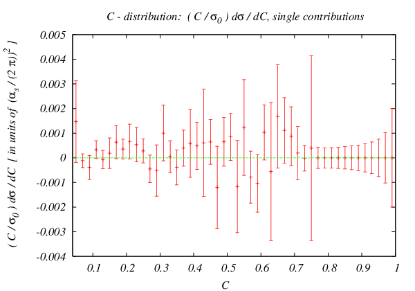
Refer to caption
Refer to caption
Refer to caption
Refer to caption
Refer to caption
Refer to caption
Figure 3: From top to bottom: Comparison of the contribution proportional to NC​CF​nf​TR,NC2​CF,NC​CF2N_{C}\,C_{F}\,n_{f}\,T_{R},\;N_{C}^{2}\,C_{F},\;N_{C}\,C_{F}^{2} for our scheme (NS) and Catani Seymour dipoles (CS). Shown is the differential distribution Cσ0​d​σNLOd​C\frac{C}{\sigma_{0}}\,\frac{d\sigma^{\text{NLO}}}{dC} in units of (αs2​π)2\left(\frac{\alpha_{s}}{2\,\pi}\right)^{2}, with C defined by Eqn.(93). Left: Results for the implementation of our scheme and Catani Seymour subtraction terms from our private code as well as event2_\_3.f [84]. Right: Relative difference between our implementation of the CS and NS subtraction terms. The results agree on the percent level and are consistent with zero within the integration errors. Large errors arise in regions where the absolute values of the differential distribution become small.
Refer to caption
Figure 4: Total result for differential distribution Cσ0​d​σNLOd​C\frac{C}{\sigma_{0}}\,\frac{d\sigma^{\text{NLO}}}{dC} using both NS (red) and CS (green) dipoles. The standard literature result obtained using the CS scheme is completely reproduced with the NS dipoles.
Refer to caption
Figure 5: Differences ΔCS-NS\Delta_{\text{CS-NS}} for real emission (red, upper) and virtual (green, lower) virtual contributions, showing that especially for low CC values the contributions in the two schemes significantly differ. Adding up Δreal+Δvirt\Delta^{\text{real}}+\Delta^{\text{virt}} gives 0 as expected.

Results for integration as well as differential distributions have been obtained using routines from the Cuba library [86].

5 Conclusion and Outlook

In this work, we have extended the alternative subtraction scheme for NLO QCD calculations proposed in [52, 53, 54] to the case of an arbitrary number of massless partons in the final state. The scheme employs a momentum mapping that reduces the number of reevaluations of the underlying Born matrix element with respect to standard schemes [59, 64] 1414 14 We want to note that the Frixione-Kunszt-Signer (FKS) subtraction scheme [58] exhibits a scaling behaviour similar to our scheme. However, the two prescriptions differ in the treatment of phase space setup; in addition, no parton shower proposal exists using FKS splitting functions. We thank R. Frederix for helpful discussions regarding this point.. Furthermore, the use of subtraction terms based on the shower splitting functions promises to facilitate the matching of parton-level NLO corrections with the improved parton shower1515 15 For an explicit discussion on this, see eg [50, 87], where the authors additionally emphasize that in case of processes with subleading colour divergences, this choice naturally allows to sustain NLO accuracy of total and differential distributions after matching with the shower. We thank S. Höche for valuable comments regarding this.. We provide formulae for the corresponding final state subtraction terms and their integrated counterparts. We validate our expressions by reproducing the literature results for the differential distribution of the CC parameter at NLO for three jet production at lepton colliders, where we find numerical agreement between results from the implementation of our scheme and two independent implementations of the Catani Seymour scheme on the (sub)percent level. Combining the results in this work with the discussion in [52, 53, 54] provides all formulae needed for a generic application of our scheme for massless emitters, and therefore concludes the discussion of the subtraction scheme in the massless case.

As argued in the Introduction, subtraction schemes can generically differ in the nonsingular structure of the dipole subtraction terms as well as the mapping between real emission and Born-type kinematics, which guarantees on-shellness and energy momentum conservation in both phase spaces. The scheme adopted here uses the whole remaining event as a spectator for the mapping, thereby leading to a scaling behaviour of Born reevaluations ∼N2/2\sim\,N^{2}/2, where NN is the number of final state partons. However, this simplified mapping equally induces integrated subtraction terms with finite parts that exhibit a non-trivial dependence on the integration parameters of the unresolved one-parton phase space. In this work, we chose to evaluate these finite terms numerically, which leads to an increase of integration variables by two in the numerical implementation of the scheme. However, recently it was proposed [1] to approximate similar finite terms by polynomial functions in the context of a next-to-next-to-leading order subtraction scheme[88, 89, 90, 91]. We therefore plan to make the finite remainders that appear in the integrated subtraction terms available either in form of approximating functions or a librarized grid interpolating between different input parameters for aℓa_{\ell}. Further plans for future work include the extension to the massive scheme as well as the matching with the improved parton shower1616 16 The scheme presented here has recently been implemented into the Helac NLO event Generator framework [15, 92]. .

Acknowledgements

This research was partially supported by the DFG SFB/TR9 “Computational Particle Physics”, the DFG Graduiertenkolleg “Elementary Particle Physics at the TeV Scale”, the Helmholtz Alliance “Physics at the Terascale” and the BMBF. We would like to thank Zoltán Nagy, Dave Soper, Zoltán Trócsányi, Michael Krämer and Gabor Somogyi for many valuable discussions, as well as Tobias Huber for help with integrations including HypExp and Mike Seymour for help with his code for e​e→ 3ee\,\rightarrow\,3 jets. In addition, C.H.C wants to thank Alexander Mück and Michael Kubocz for useful discussions. T.R. thanks Thomas Hahn for useful comments regarding the Cuba library, Stefan Höche and Rikkert Frederix for useful comments on NLO and parton shower matching and the FKS implementation in Madgraph respectively, as well as Christoph Gnendiger for helpful comments regarding the manuscript. T.R. equally acknowledges financial support by the SFB 676 ”Particles, strings, and the early universe” during the final stages of this work.

Appendix A Splitting amplitudes

In Table 1, we list the splitting amplitudes for final state q​q¯​gq\bar{q}g splittings as given in [74].

ℓ\ell fℓf_{\ell} f^ℓ\hat{f}_{\ell} f^j\hat{f}_{j} vℓ×14​π​αs\displaystyle{v_{\ell}\times\frac{1}{\sqrt{4\pi\alpha_{s}}}} colour
FF qq qq g εμ​(p^j,s^j,Q^)∗​U¯​(p^ℓ,s^ℓ)​γμ​[/p^ℓ+/p^j]​/nℓ​U​(pℓ,sℓ)2​pℓ⋅nℓ​[(p^ℓ+p^j)2]\displaystyle{\varepsilon_{\mu}(\hat{p}_{j},\hat{s}_{j};\hat{Q})^{*}\,\frac{\overline{U}({\hat{p}_{\ell},\hat{s}_{\ell}})\gamma^{\mu}[{\raise 1.11111pt\hbox to5.55557pt{\hss/\hss}\hbox to0.0pt{\hss$\hat{p}$}}_{\ell}+{\raise 1.11111pt\hbox to5.55557pt{\hss/\hss}\hbox to0.0pt{\hss$\hat{p}$}}_{j}]{\raise-1.09723pt\hbox to9.84961pt{\hss/\hss}\hbox to0.0pt{\hss$n_{\ell}$}}U({p_{\ell},s_{\ell}})}{2p_{\ell}\!\cdot\!n_{\ell}\ [(\hat{p}_{\ell}+\hat{p}_{j})^{2}]}} tat^{a}
FF g qq q¯\bar{q} −εμ​(pℓ,sℓ,Q^)​Dμ​ν​(p^ℓ+p^j,nℓ)​U¯​(p^ℓ,s^ℓ)​γν​V​(p^j,s^j)(p^ℓ+p^j)2\displaystyle{-\varepsilon^{\mu}(p_{\ell},s_{\ell};\hat{Q})D_{\mu\nu}(\hat{p}_{\ell}+\hat{p}_{j},n_{\ell})\frac{\overline{U}({\hat{p}_{\ell},\hat{s}_{\ell}})\gamma^{\nu}V({\hat{p}_{j},\hat{s}_{j})}}{(\hat{p}_{\ell}+\hat{p}_{j})^{2}}} tat^{a}
Table 1: Splitting amplitudes vℓ​({p^,f^}j,s^j,s^ℓ,sℓ)v_{\ell}(\{\hat{p},\hat{f}\}_{j},\hat{s}_{j},\hat{s}_{\ell},s_{\ell}) involving a q​q¯​gq\bar{q}g splitting. We have removed a common factor 4​π​αs\sqrt{4\pi\alpha_{s}}. The label ℓ\ell denotes final state indices F={1,…,m}F=\{1,\dots,m\}. The lightlike vector nℓn_{\ell} is defined in Eqn. (96). Taken from [74].

For triple gluon splittings, we have for the final state

vℓ({p^,f^}m+1,OPENs^j,s^ℓ,sℓ)=4​π​αs2​p^j⋅p^ℓ​εα​(p^j,s^j,Q^)∗​εβ​(p^ℓ,s^l,Q^)∗​εν​(pℓ,sℓ,Q^)×vα​β​γ​(p^j,p^ℓ,−p^j−p^ℓ)​Dγ​ν​(p^ℓ+p^j,nℓ).\begin{split}v_{\ell}(\{\hat{p},\hat{f}\}_{m+1},&\hat{s}_{j},\hat{s}_{\ell},s_{\ell})\\ &=\frac{\sqrt{4\pi\alpha_{s}}}{2\hat{p}_{j}\!\cdot\!\hat{p}_{\ell}}\,\varepsilon_{\alpha}(\hat{p}_{j},\hat{s}_{j};\hat{Q})^{*}\varepsilon_{\beta}(\hat{p}_{\ell},\hat{s}_{l};\hat{Q})^{*}\varepsilon^{\nu}(p_{\ell},s_{\ell};\hat{Q})\\ &\quad\times v^{\alpha\beta\gamma}(\hat{p}_{j},\hat{p}_{\ell},-\hat{p}_{j}-\hat{p}_{\ell})\,D_{\gamma\nu}(\hat{p}_{\ell}+\hat{p}_{j};n_{\ell})\,.\end{split} (94)

We use standard notation where U⁡(p,s),U¯​(p,s),V⁡(p,s),V¯​(p,s)U(p,s),\overline{U}(p,s),V(p,s),\overline{V}(p,s) denote spinors of the fermions with a four-momentum pp and spin ss, and εα​(p,s,Q)\varepsilon_{\alpha}(p,s;Q) are the gluon polarisation vectors. The g​g​gggg vertex has the form

vα​β​γ​(pa,pb,pc)=gα​β​(pa−pb)γ+gβ​γ​(pb−pc)α+gγ​α​(pc−pa)β.v^{\alpha\beta\gamma}(p_{a},p_{b},p_{c})=g^{\alpha\beta}(p_{a}-p_{b})^{\gamma}+g^{\beta\gamma}(p_{b}-p_{c})^{\alpha}+g^{\gamma\alpha}(p_{c}-p_{a})^{\beta}\,. (95)

The transverse projection tensor Dγ​ν​(p^ℓ−p^j,nℓ)D_{\gamma\nu}(\hat{p}_{\ell}-\hat{p}_{j};n_{\ell}) is defined according to Eqn. (3.1.1). The lightlike vector nℓn_{\ell} is given by

nℓ=Q−Q2Q⋅pℓ+(Q⋅pℓ)2​pℓ,ℓ∈{1,…,m}.n_{\ell}=Q-\frac{Q^{2}}{Q\!\cdot\!p_{\ell}+\sqrt{(Q\!\cdot\!p_{\ell})^{2}}}\ p_{\ell}\;\;,\ell\in\{1,\dots,m\}\;\;. (96)

Appendix B Incoming hadrons

In case of processes with two initial-state hadrons AA and BB carrying momenta pAp_{A} and pBp_{B}, respectively, the calculation of the QCD cross sections must be convoluted with parton distribution functions fi/I​(ηi,μF2)f_{i/I}(\eta_{i},\mu^{2}_{F}) which depends on the factorization scale μF\mu_{F}:

σ⁡(pA,pB)\displaystyle\sigma(p_{A},p_{B}) =∑a,b∫01d​ηa​fa/A​(ηa,μF2)​∫01d​ηb​fb/B​(ηb,μF2)​[σa​bLO​(pa,pb)+σa​bNLO​(pa,pb,μF2)]\displaystyle=\,\sum_{a,\,b}\int_{0}^{1}d\eta_{a}\,f_{a/A}(\eta_{a},{\mu_{F}^{2}})\int_{0}^{1}d\eta_{b}\,f_{b/B}(\eta_{b},{\mu_{F}^{2}})\left[\sigma^{\text{LO}}_{ab}(p_{a},p_{b})+\sigma^{\text{NLO}}_{ab}(p_{a},p_{b},\mu_{F}^{2})\right] (97)

where pa=ηa​pAp_{a}\,=\,\eta_{a}\,p_{A} and pb=ηb​pBp_{b}\,=\,\eta_{b}\,p_{B} are parton momenta, while ηa\eta_{a} and ηb\eta_{b} are the momentum fractions of the partons. In this case, additional collinear counterterms need to be added to the integrated subtraction terms1717 17 C.f. e.g. [93]., and the parton level NLO contribution becomes

σa​bNLO​(pa,pb,μF2)\displaystyle\sigma^{\text{NLO}}_{ab}(p_{a},p_{b},\mu_{F}^{2}) =∫m+1d​σa​bR​(pa,pb)+∫md​σa​bV​(pa,pb)+∫md​σa​bC​(pa,pb,μF2).\displaystyle=\int_{m+1}d\sigma^{R}_{ab}(p_{a},p_{b})+\int_{m}d\sigma^{V}_{ab}(p_{a},p_{b})+\int_{m}d\sigma^{C}_{ab}(p_{a},p_{b},\mu_{F}^{2}). (98)

We then have

σa​bNLO​(pa,pb,μF2)\displaystyle\sigma_{ab}^{\text{NLO}}(p_{a},p_{b},\mu_{F}^{2}) =∫m+1[d​σa​bR​(pa,pb)−d​σa​bA​(pa,pb)]\displaystyle=\int_{m+1}\left[d\sigma_{ab}^{R}(p_{a},p_{b})-d\sigma_{ab}^{A}(p_{a},p_{b})\right]
+∫m[∫dσa​bV(pa,pb)+∫1dσa​bA(pa,pb)+dσa​bC(pa,pb,μF2)]ε=0,\displaystyle+\int_{m}\,\left[\int d\sigma^{V}_{ab}(p_{a},p_{b})+\int_{1}d\sigma^{A}_{ab}(p_{a},p_{b})+d\sigma_{ab}^{C}(p_{a},p_{b},\mu_{F}^{2})\right]_{\varepsilon=0}, (99)

with

∫m[∫1d​σa​bA​(pa,pb)+d​σa​bC​(pa,pb,μF2)]\displaystyle\int_{m}\left[\int_{1}d\sigma^{A}_{ab}(p_{a},p_{b})+d\sigma^{C}_{ab}(p_{a},p_{b},\mu_{F}^{2})\right]
=\displaystyle= ∫md​σa​bB​(pa,pb)⊗I⁡(ε)+∫01d​x​∫md​σa​bB​(x​pa,pb)⊗[Ka​(x​pa)+P⁡(x,μF2)]\displaystyle\int_{m}d\sigma_{ab}^{B}(p_{a},p_{b})\otimes{I}(\varepsilon)+\int_{0}^{1}dx\int_{m}d\sigma_{ab}^{B}(xp_{a},p_{b})\otimes\left[{K}^{a}(xp_{a})+{P}(x,\mu_{F}^{2})\right]
+\displaystyle+ ∫01d​x​∫md​σa​bB​(pa,x​pb)⊗[Kb​(x​pb)+P⁡(x,μF2)].\displaystyle\int_{0}^{1}dx\int_{m}d\sigma_{ab}^{B}(p_{a},xp_{b})\otimes\left[{K}^{b}(xp_{b})+{P}(x,\mu_{F}^{2})\right]. (100)

This equation defines the insertion operators I⁡(ε),K⁡(x),P⁡(x,μF2)I(\varepsilon),\,K(x),\,P(x;\mu_{F}^{2}) on an integrated cross section level. Eqn. (100) can be divided into two parts: the first part is the universal insertion operator I⁡(ε){I}(\varepsilon), which contains the complete singularity structure of the virtual contribution and has LO kinematics. The second part consists of the finite pieces that are left over after absorbing the initial-state collinear singularities into a redefinition of the parton distribution functions at NLO. It involves an additional one-dimensional integration over the momentum fraction xx of an incoming parton with the LO cross sections and the xx-dependent structure functions.

In the MS¯\overline{\textrm{MS}} scheme, the collinear counterterms are given by

∫md​σa​bC​(pa,pb,μF2)\displaystyle\int_{m}d\sigma^{C}_{ab}(p_{a},p_{b},\mu_{F}^{2}) =αs2​π​1Γ⁡(1−ε)​∑c∫01d​x​∫md​σc​bB​(x​pa,pb)​1ε​(4​π​μ2μF2)ε​Pa​c​(x)\displaystyle=\frac{\alpha_{s}}{2\pi}\,\frac{1}{\Gamma(1-\varepsilon)}\,\sum_{c}\int_{0}^{1}dx\int_{m}d\sigma_{cb}^{B}(xp_{a},p_{b})\,\frac{1}{\varepsilon}\,\left(\frac{4\pi\mu^{2}}{\mu_{F}^{2}}\right)^{\varepsilon}\,P^{ac}(x)
+αs2​π1Γ⁡(1−ε)∑c∫01dx∫mdσa​cB(pa,xpb)1ε(4​π​μ2μF2)εPb​c(x).\displaystyle+\frac{\alpha_{s}}{2\pi}\,\frac{1}{\Gamma(1-\varepsilon)}\,\sum_{c}\int_{0}^{1}dx\int_{m}d\sigma_{ac}^{B}(p_{a},xp_{b})\,\frac{1}{\varepsilon}\,\left(\frac{4\pi\mu^{2}}{\mu_{F}^{2}}\right)^{\varepsilon}\,P^{bc}(x). (101)

Here the Pa​b​(x)P^{ab}(x) are the Altarelli-Parisi kernels in four dimensions [71], which are evolution kernels of the DGLAP equation [94, 95, 71, 96], and describe the behaviour of parton splittings by giving the probability of finding a parton of type bb with momentum fraction xx in a parton of type aa in the collinear limit:

a⁡(p)⟶b⁡(x​p+k⟂+𝒪⁡(k⟂2))+c⁡((1−z)​p−k⟂+𝒪⁡(k⟂2)).a(p)\,\longrightarrow\,b\left(x\,p+k_{\perp}+\,\mathcal{O}(k_{\perp}^{2})\right)\,+\,c\,\left((1-z)\,p-k_{\perp}+\,\mathcal{O}(k_{\perp}^{2})\right). (102)

At leading order, the splitting functions are given by

Pq​q​(x)\displaystyle P^{qq}(x) =\displaystyle= CF​[1+x2(1−x)++32​δ​(1−x)],\displaystyle C_{F}\,\left[\frac{1+x^{2}}{(1-x)_{+}}+\frac{3}{2}\,\delta(1-x)\right],
Pg​q​(x)\displaystyle P^{gq}(x) =\displaystyle= TR​[x2+(1−x)2],TR=12,\displaystyle T_{R}\,\left[x^{2}+(1-x)^{2}\right],\;T_{R}\,=\,\frac{1}{2},
Pq​g​(x)\displaystyle P^{qg}(x) =\displaystyle= CF​[1+(1−x)2x],\displaystyle C_{F}\,\left[\frac{1+(1-x)^{2}}{x}\right],
Pg​g​(x)\displaystyle P^{gg}(x) =\displaystyle= 2​CA​[x(1−x)++1−xx+x⁡(1−x)]+δ⁡(1−x)​11​CA−4​nf​TR6,\displaystyle 2\,C_{A}\,\left[\frac{x}{(1-x)_{+}}\,+\,\frac{1-x}{x}+x\,(1-x)\right]+\delta(1-x)\,\frac{11\,C_{A}-4\,n_{f}\,T_{R}}{6}\,,

where nfn_{f} is the number of quark flavours in the theory. The ++ distribution is defined in the standard way

∫01f⁡(x)​g+​(x)​𝑑x=∫01g⁡(x)​(f⁡(x)−f⁡(1))​𝑑x=∫01g⁡(x)​f​(x)​𝑑x−f⁡(1)​∫01g⁡(x)​𝑑x\int^{1}_{0}\,f(x)\,g_{+}(x)\,dx\,=\,\int^{1}_{0}\,g(x)\,(f(x)-f(1))\,dx\,=\,\int^{1}_{0}\,g(x)\,f(x)\,dx\,-\,f(1)\,\int^{1}_{0}g(x)\,dx (104)

for the convolution with a test function f⁡(x)f(x).

Appendix C Four-particle phase space

In this section, we derive the parametrization that was used for the real emission phase space in Section 4. We use the standard notation for an nn-parton phase space in four dimensions:

d​Γn=∏i[d4​pi(2​π)4​δ​(pi2−mi2)]​δ(4)​(pin−∑ipi).d\Gamma_{n}\,=\,\prod_{i}\,\left[\frac{d^{4}p_{i}}{(2\pi)^{4}}\,\delta\left(p_{i}^{2}-m_{i}^{2}\right)\right]\,\delta^{(4)}\left(p_{\text{in}}-\sum_{i}\,p_{i}\right).

We build our parametrization from a successive chain with

pin→p12+p34,pi​j→pi+pj,p_{\text{in}}\,\rightarrow\,p_{12}+p_{34},\,p_{ij}\,\rightarrow\,p_{i}+p_{j},

where in the first step the on-shell condition for pi​jp_{ij} needs to be replaced by a distribution of si​j=(pi+pj)2s_{ij}\,=\,(p_{i}+p_{j})^{2}.

Generic massive two parton phase space, center-of-mass system

For a generic massive two parton phase space, we use the following parametrization in the center-of-mass system

d​Γ2=132​π2​λ⁡(s,m12,m22)s​d​Ω1​Θ​(s−(m1+m2)),d\Gamma_{2}\,=\,\frac{1}{32\,\pi^{2}}\,\frac{\sqrt{\lambda(s,m_{1}^{2},m_{2}^{2})}}{s}d\Omega_{1}\,\Theta\left(\sqrt{s}-(m_{1}+m_{2})\right),

where

p10=s+m12−m222​s,|p→1|=λ⁡(s,m12,m22)2​s,p2=pin−p1.p_{1}^{0}\,=\,\frac{s+m_{1}^{2}-m_{2}^{2}}{2\,\sqrt{s}},\,|\overrightarrow{p}_{1}|\,=\,\frac{\sqrt{\lambda(s,m_{1}^{2},m_{2}^{2})}}{2\,\sqrt{s}},\,p_{2}\,=\,p_{\text{in}}-p_{1}.

The Θ\Theta function arises from the conditions Θ⁡(|p→1|)​Θ​(|p→2|)\Theta(|\overrightarrow{p}_{1}|)\,\Theta(|\overrightarrow{p}_{2}|). λ\lambda is defined as

λ⁡(x1,x2,x3)=∑ixi2−2​∑i>jxi​xj.\lambda(x_{1},x_{2},x_{3})\,=\,\sum_{i}\,x_{i}^{2}-2\,\sum_{i\,>\,j}x_{i}x_{j}.

Generic massless two parton phase space, non-center-of-mass system

If we consider two partons in a non-center-of-mass system, with

pin=(Ein00|p→in|)p_{\text{in}}\,=\,\left(\begin{array}[]{c}E_{\text{in}}\\ 0\\ 0\\ |\overrightarrow{p}_{\text{in}}|\end{array}\right)

i.e. where the three vector of pinp_{\text{in}} determines the z axis, we obtain for a two parton massless phase space

d​Γ2=116​π2​|p→in|​d​p10​d​ϕ1,d\Gamma_{2}\,=\,\frac{1}{16\,\pi^{2}\,|\overrightarrow{p}_{\text{in}}|}dp_{1}^{0}\,d\phi_{1},

where we have

cos⁡θ1=1|p→in|​(Ein−min22​p10)\cos\theta_{1}\,=\,\frac{1}{|\overrightarrow{p}_{\text{in}}|}\left(E_{\text{in}}-\frac{m^{2}_{\text{in}}}{2\,p_{1}^{0}}\right) (105)

and

min22​(Ein+|p→in|)≤p10≤min22​(Ein−|p→in|)\frac{m^{2}_{\text{in}}}{2\,(E_{\text{in}}+|\overrightarrow{p}_{\text{in}}|)}\,\leq\,p^{0}_{1}\,\leq\,\frac{m^{2}_{\text{in}}}{2\,(E_{\text{in}}-|\overrightarrow{p}_{\text{in}}|)}

from the requirement that |cos⁡θ1|≤ 1|\cos\theta_{1}|\leq\,1. In this derivation,

p1,z=p10cosθ1.p_{1,z}\,=\,p_{1}^{0}\,\cos\theta_{1}.

If the z-component of pinp_{\text{in}} goes into the negative zz-direction, cos⁡θ→−cos⁡θ\cos\theta\,\rightarrow\,-\cos\theta in Eqn. (105), and all other above relations still hold.

Generic four parton phase space with massless final states

We use the generic expression

d​Γn​(X→∑pn)=d​ΓX→Y+Z​d​mX22​π​d​mY22​π​d​ΓX→∑po​d​ΓY→∑po′,d\Gamma_{n}\,\left(X\rightarrow\,\sum p_{n}\right)\,=\,d\Gamma_{X\rightarrow\,Y+Z}\,\frac{dm^{2}_{X}}{2\pi}\,\frac{dm^{2}_{Y}}{2\pi}\,d\Gamma_{X\rightarrow\,\sum p_{o}}\,d\Gamma_{Y\rightarrow\,\sum p_{o}^{\prime}},

where ∑po+∑po′=∑pn\sum p_{o}\,+\,\sum p_{o}^{\prime}\,=\,\sum p_{n} is the sum over all nn outgoing particles. Using the expressions above as well as

yi​j=si​js,xi= 2​pi⋅Qs,y_{ij}\,=\,\frac{s_{ij}}{s},\,x_{i}\,=\,2\frac{p_{i}\cdot Q}{s},

we obtain for the four-parton phase space in the center-of-mass system of pin≡Qp_{\text{in}}\,\equiv\,Q:

d​Γ4=s2(4​π)6​λ⁡(1,y12,y34)​d​y12​d​y34​d​x1​d​x3​d​ϕ3,d\Gamma_{4}\,=\,\frac{s^{2}}{(4\,\pi)^{6}\,\sqrt{\lambda(1,y_{12},y_{34})}}\,dy_{12}\,dy_{34}\,dx_{1}\,dx_{3}\,d\phi_{3},

with the four-vectors

p12=(EX00pX),p34=(EY00−pX),\displaystyle p_{12}\,=\,\left(\begin{array}[]{c}E_{X}\\ 0\\ 0\\ p_{X}\end{array}\right),\;p_{34}\,=\,\left(\begin{array}[]{c}E_{Y}\\ 0\\ 0\\ -p_{X}\end{array}\right),
p1=x1​s2​(1sin⁡θ10cos⁡θ1),p3=x3​s2​(1sinθ3cosϕ3sinθ3sinϕ3cos⁡θ3),\displaystyle p_{1}\,=\,x_{1}\,\frac{\sqrt{s}}{2}\,\left(\begin{array}[]{c}1\\ \sin\theta_{1}\\ 0\\ \cos\theta_{1}\end{array}\right),\;p_{3}\,=\,x_{3}\,\frac{\sqrt{s}}{2}\,\left(\begin{array}[]{c}1\\ \sin\theta_{3}\,\cos\phi_{3}\\ \sin\theta_{3}\sin\phi_{3}\\ \cos\theta_{3}\end{array}\right),
p2=p12−p1,p4=p34−p3,\displaystyle p_{2}\,=\,p_{12}-p_{1},\;p_{4}\,=\,p_{34}-p_{3},

and where

EX=s2​(1+y12−y34),pX=s​λ​(1,y12,y34)2,\displaystyle E_{X}\,=\,\frac{\sqrt{s}}{2}\left(1+y_{12}-y_{34}\right),\,p_{X}\,=\,\frac{\sqrt{s\,\lambda(1,y_{12},y_{34})}}{2},
EY=s−EX=s2​(1+y34−y12),\displaystyle E_{Y}\,=\,\sqrt{s}-E_{X}\,=\,\frac{\sqrt{s}}{2}\left(1+y_{34}-y_{12}\right),
cos⁡θ1=1pX​(EX−mX2x1​s)=1λ⁡(1,y12,y34)​(1+y12−y34−2​y12x1),\displaystyle\cos\theta_{1}\,=\,\frac{1}{p_{X}}\left(E_{X}-\frac{m^{2}_{X}}{x_{1}\,\sqrt{s}}\right)\,=\,\frac{1}{\sqrt{\lambda(1,y_{12},y_{34})}}\,\left(1+y_{12}-y_{34}-\frac{2\,y_{12}}{x_{1}}\right),
cos⁡θ3=−1pX​(EY−mY2x3​s)=−1λ⁡(1,y12,y34)​(1+y34−y12−2​y34x3).\displaystyle\cos\theta_{3}\,=\,-\frac{1}{p_{X}}\left(E_{Y}-\frac{m^{2}_{Y}}{x_{3}\,\sqrt{s}}\right)\,=\,-\frac{1}{\sqrt{\lambda(1,y_{12},y_{34})}}\,\left(1+y_{34}-y_{12}-\frac{2\,y_{34}}{x_{3}}\right).\

The integration boundaries are given by

y34≤(1−y12)2,\displaystyle y_{34}\,\leq\,\left(1-\sqrt{y_{12}}\right)^{2},
x1min/max=mX2s​(EX±pX)=2​y121−y12+y34±λ⁡(1,y12,y34),\displaystyle x_{1}^{\text{min/max}}\,=\,\frac{m_{X}^{2}}{\sqrt{s}\,\left(E_{X}\,\pm\,p_{X}\right)}\,=\,\frac{2\,y_{12}}{1-y_{12}+y_{34}\,\pm\,\sqrt{\lambda(1,y_{12},y_{34})}},
x3min/max=mY2s​(EY±pX)=2​y341−y34+y12±λ⁡(1,y12,y34).\displaystyle x_{3}^{\text{min/max}}\,=\,\frac{m_{Y}^{2}}{\sqrt{s}\,\left(E_{Y}\,\pm\,p_{X}\right)}\,=\,\frac{2\,y_{34}}{1-y_{34}+y_{12}\,\pm\,\sqrt{\lambda(1,y_{12},y_{34})}}.

Appendix D Note on further possible scaling improvement

As argued in Section 3.4, the scheme discussed here exhibits a scaling behaviour for the reevaluation of the underlying Born matrix element proportional to N2N^{2}, with NN being the number of final state particles in the corresponding real emission process. The same scaling behaviour is implicit in the FKS scheme [58], where the mapping of the Born-type matrix element is transferred to the explicit parametrization of phase space for each emitter/ emitted parton pair. In [69], it was shown that within this scheme the scaling behaviour can be reduced to a constant for processes containing symmetric final states. In the following, we want to argue that exactly the same scaling behaviour can be achieved in the scheme discussed here and is indeed implicit in the setup of our scheme, and especially the choice of soft interference terms proposed in Section 3.1.2. The implementation of this prescription in a numerical code is in the line of future work.

The improved scaling behaviour proposed in [69] relies on the fact that any m+1m+1 phase space can be decomposed into disjoint partitions of phase space that are specified by their behaviour for one of the partons p^i\hat{p}_{i} becoming soft or collinear to at most one additional parton p^j\hat{p}_{j}: these adjoint pairs are then denoted FKS pairs, where the sum of all subspace partitions reproduces the whole phase space1818 18 Note that the notation between [69] and this work differs in the fact that in [69], p^i\hat{p}_{i} labels the emitted parton that becomes soft or collinear, while in our case this parton is denoted by p^j\hat{p}_{j}. For sake of consistency, we here stick to the notation proposed in [69]. :

∑(i,j)∈𝒫FKS𝒮i​j= 1\sum_{(i,j)\in\mathcal{P}_{\text{FKS}}}\,\mathcal{S}_{ij}\,=\,1

(Eqn (4.16) in [69]), where 𝒫FKS\mathcal{P}_{\text{FKS}} denotes the set of FKS partitions. Furthermore, the authors observe that for processes displaying symmetries in the final state, which are subsequently reflected in the matrix element and phase space, several partitions 𝒮i​j\mathcal{S}_{ij} render exactly the same contribution to the final observable, and that therefore the evaluation of at most one of these is sufficient, the others being related by symmetry:

d​σ(n+1)​(r)=∑(i,j)∈𝒫¯FKSξi​j(n+1)​(r)​d​σi​j(n+1)​(r),d\sigma^{(n+1)}(r)\,=\,\sum_{(i,j)\in\overline{\mathcal{P}}_{\text{FKS}}}\xi_{ij}^{(n+1)}(r)d\sigma_{ij}^{(n+1)}(r), (108)

(eqn (6.7) in [69]), where ξi​j(n+1)​(r)\xi_{ij}^{(n+1)}(r) denotes the process-dependent symmetry factor that relates the total cross section to the one evaluated in the partition denoted by 𝒮i​j\mathcal{S}_{ij}, and 𝒫¯FKS\overline{\mathcal{P}}_{\text{FKS}} now denotes the set of all nonredundant partitions. Note that an important argument here is that all other contributions that stem from p^i\hat{p}_{i} becoming soft, but collinear to a different parton p^k\hat{p}_{k}, belong to a different partition 𝒮i​k\mathcal{S}_{ik} and are therefore suppressed via the structure of 𝒮i​j\mathcal{S}_{ij}. Especially for purely gluonic final states, 𝒫¯FKS\overline{\mathcal{P}}_{\text{FKS}} contains only one element.

In the scheme discussed here, the subtraction term that reflects the divergences of 𝒮i​j\mathcal{S}_{ij} is given by Eqn. (67):

𝒟⁡(p^j,p^i)=𝒟coll​(p^j,p^i)+δf^j,g​∑k≠(i,j)𝒟if​(p^j,p^i,p^k);{\mathcal{D}}(\hat{p}_{j},\hat{p}_{i})\,=\,\mathcal{D}^{\text{coll}}(\hat{p}_{j},\hat{p}_{i})\,+\,\delta_{\hat{f}_{j},g}\sum_{k\,\neq\,(i,j)}\mathcal{D}^{\text{if}}(\hat{p}_{j},\hat{p}_{i},\,\hat{p}_{k});

as discussed in Section 3.1.2, all contributions from the soft/collinear divergence of p^i,p^k\hat{p}_{i},\,\hat{p}_{k} are transferred to the interference term 𝒟if​(p^k,p^i,p^j)\mathcal{D}^{\text{if}}(\hat{p}_{k},\hat{p}_{i},\,\hat{p}_{j}), corresponding to the singularity structure of a different partition, namely 𝒮i​k\mathcal{S}_{ik}. All terms in Eqn. (67) come with the same mapping, and, as in the FKS prescription in [69], only the set of nonredundant contributions needs to be evaluated, all others being related by symmetry. Increasing the number of final state gluons then leads to a change in the constant ξi​j(n+1)​(r)\xi_{ij}^{(n+1)}(r) but does not call for the evaluation of a larger number of nonredundant contributions, as the number of elements in 𝒫¯FKS\overline{\mathcal{P}}_{\text{FKS}} remains constant. Therefore, following this prescription, our scheme equally exhibits a constant scaling behaviour, when the number of gluons in the real emission final state is increased.

We finally want to comment that, although the above prescription can naturally lead to a significant improvement in the treatment of real-emission subtractions for multi-parton final states, it is not straightforward to implement in standard Monte Carlo generators that do not internally make use of the symmetries exhibited in Eqn. (108). The implementation of this prescription therefore equally calls for a modification of the NLO tools used for calculating the corresponding process.

References

  • [1] J. Alcaraz Maestre, S. Alioli, J.R. Andersen, R.D. Ball, A. Buckley, et al. The SM and NLO Multileg and SM MC Working Groups: Summary Report. 2012.
  • [2] http://mcfm.fnal.gov.
  • [3] http://www.desy.de/∼\simznagy/Site/NLOJet++.html.
  • [4] K. Arnold et al. VBFNLO: A parton level Monte Carlo for processes with electroweak bosons. Comput. Phys. Commun., 180:1661–1670, 2009.
  • [5] K. Arnold, J. Bellm, G. Bozzi, M. Brieg, F. Campanario, et al. VBFNLO: A parton level Monte Carlo for processes with electroweak bosons – Manual for Version 2.5.0. 2011.
  • [6] R. Keith Ellis, W. T. Giele, and G. Zanderighi. Semi-numerical evaluation of one-loop corrections. Phys. Rev., D73:014027, 2006.
  • [7] Richard Keith Ellis. An update on the next-to-leading order Monte Carlo MCFM. Nucl.Phys.Proc.Suppl., 160:170–174, 2006.
  • [8] Z. Bern, G. Diana, L.J. Dixon, F. Febres Cordero, S. Hoeche, et al. Four-Jet Production at the Large Hadron Collider at Next-to-Leading Order in QCD. Phys.Rev.Lett., 109:042001, 2012.
  • [9] H. Ita, Z. Bern, L.J. Dixon, Fernando Febres Cordero, D.A. Kosower, et al. Precise Predictions for Z + 4 Jets at Hadron Colliders. Phys.Rev., D85:031501, 2012.
  • [10] C.F. Berger, Z. Bern, Lance J. Dixon, F. Febres Cordero, D. Forde, et al. Precise Predictions for W + 4 Jet Production at the Large Hadron Collider. Phys.Rev.Lett., 106:092001, 2011.
  • [11] C. F. Berger et al. Precise Predictions for WW + 3 Jet Production at Hadron Colliders. Phys. Rev. Lett., 102:222001, 2009.
  • [12] C. F. Berger et al. Next-to-Leading Order QCD Predictions for W+3-Jet Distributions at Hadron Colliders. Phys. Rev., D80:074036, 2009.
  • [13] Nicolas Greiner, Alberto Guffanti, Thomas Reiter, and Jurgen Reuter. NLO QCD corrections to the production of two bottom-antibottom pairs at the LHC. Phys.Rev.Lett., 107:102002, 2011.
  • [14] T. Binoth et al. Next-to-leading order QCD corrections to pp →b​b¯​b\rightarrow\,b\,\bar{b}\,b b¯\bar{b} + X at the LHC: the quark induced case. Phys. Lett., B685:293–296, 2010.
  • [15] G. Bevilacqua, M. Czakon, M.V. Garzelli, A. van Hameren, A. Kardos, et al. HELAC-NLO. Comput.Phys.Commun., 184:986–997, 2013.
  • [16] G. Bevilacqua, M. Czakon, C.G. Papadopoulos, and M. Worek. Hadronic top-quark pair production in association with two jets at Next-to-Leading Order QCD. Phys.Rev., D84:114017, 2011.
  • [17] Giuseppe Bevilacqua, Michal Czakon, Andreas van Hameren, Costas G. Papadopoulos, and Malgorzata Worek. Complete off-shell effects in top quark pair hadroproduction with leptonic decay at next-to-leading order. JHEP, 1102:083, 2011.
  • [18] G. Bevilacqua, M. Czakon, C. G. Papadopoulos, R. Pittau, and M. Worek. Assault on the NLO Wishlist: pp →\rightarrow tt bb. JHEP, 09:109, 2009.
  • [19] Stefano Frixione, Paolo Nason, and Carlo Oleari. Matching NLO QCD computations with Parton Shower simulations: the POWHEG method. JHEP, 11:070, 2007.
  • [20] Simone Alioli, Paolo Nason, Carlo Oleari, and Emanuele Re. NLO vector-boson production matched with shower in POWHEG. JHEP, 0807:060, 2008.
  • [21] Simone Alioli, Paolo Nason, Carlo Oleari, and Emanuele Re. NLO Higgs boson production via gluon fusion matched with shower in POWHEG. JHEP, 0904:002, 2009.
  • [22] Andreas Papaefstathiou and Oluseyi Latunde-Dada. NLO production of WW ’ bosons at hadron colliders using the MC@NLO and POWHEG methods. JHEP, 0907:044, 2009.
  • [23] Simone Alioli, Paolo Nason, Carlo Oleari, and Emanuele Re. NLO single-top production matched with shower in POWHEG: s- and t-channel contributions. JHEP, 0909:111, 2009.
  • [24] Paolo Nason and Carlo Oleari. NLO Higgs boson production via vector-boson fusion matched with shower in POWHEG. JHEP, 1002:037, 2010.
  • [25] Simone Alioli, Paolo Nason, Carlo Oleari, and Emanuele Re. A general framework for implementing NLO calculations in shower Monte Carlo programs: the POWHEG BOX. JHEP, 06:043, 2010.
  • [26] Stefan Hoche, Frank Krauss, Marek Schonherr, and Frank Siegert. Automating the POWHEG method in Sherpa. JHEP, 1104:024, 2011.
  • [27] Emanuele Re. Single-top Wt-channel production matched with parton showers using the POWHEG method. Eur.Phys.J., C71:1547, 2011.
  • [28] Simone Alioli, Paolo Nason, Carlo Oleari, and Emanuele Re. Vector boson plus one jet production in POWHEG. JHEP, 1101:095, 2011.
  • [29] Simone Alioli, Keith Hamilton, Paolo Nason, Carlo Oleari, and Emanuele Re. Jet pair production in POWHEG. JHEP, 1104:081, 2011.
  • [30] Carlo Oleari and Laura Reina. W±​b​b¯W^{\pm}b\bar{b} production in POWHEG. JHEP, 1108:061, 2011.
  • [31] Tom Melia, Paolo Nason, Raoul Rontsch, and Giulia Zanderighi. W+W-, WZ and ZZ production in the POWHEG BOX. JHEP, 1111:078, 2011.
  • [32] Simone Alioli, Keith Hamilton, and Emanuele Re. Practical improvements and merging of POWHEG simulations for vector boson production. JHEP, 1109:104, 2011.
  • [33] E. Bagnaschi, G. Degrassi, P. Slavich, and A. Vicini. Higgs production via gluon fusion in the POWHEG approach in the SM and in the MSSM. JHEP, 1202:088, 2012.
  • [34] Luca Barze, Guido Montagna, Paolo Nason, Oreste Nicrosini, and Fulvio Piccinini. Implementation of electroweak corrections in the POWHEG BOX: single W production. JHEP, 1204:037, 2012.
  • [35] C. Bernaciak and D. Wackeroth. Combining NLO QCD and Electroweak Radiative Corrections to W boson Production at Hadron Colliders in the POWHEG Framework. Phys.Rev., D85:093003, 2012.
  • [36] John M. Campbell, R. Keith Ellis, Rikkert Frederix, Paolo Nason, Carlo Oleari, et al. NLO Higgs boson production plus one and two jets using the POWHEG BOX, MadGraph4 and MCFM. JHEP, 1207:092, 2012.
  • [37] Emanuele Re. NLO corrections merged with parton showers for Z+2 jets production using the POWHEG method. JHEP, 1210:031, 2012.
  • [38] Michael Klasen, Karol Kovarik, Paolo Nason, and Carole Weydert. Associated production of charged Higgs bosons and top quarks with POWHEG. Eur.Phys.J., C72:2088, 2012.
  • [39] Rikkert Frederix, Emanuele Re, and Paolo Torrielli. Single-top t-channel hadroproduction in the four-flavour scheme with POWHEG and aMC@NLO. JHEP, 1209:130, 2012.
  • [40] Barbara Jager, Andreas von Manteuffel, and Stephan Thier. Slepton pair production in the POWHEG BOX. JHEP, 1210:130, 2012.
  • [41] Stefano Frixione, Eric Laenen, Patrick Motylinski, and Bryan R. Webber. Single-top production in MC@NLO. JHEP, 0603:092, 2006.
  • [42] C. Weydert, S. Frixione, M. Herquet, M. Klasen, E. Laenen, et al. Charged Higgs boson production in association with a top quark in MC@NLO. Eur.Phys.J., C67:617–636, 2010.
  • [43] Paolo Torrielli and Stefano Frixione. Matching NLO QCD computations with PYTHIA using MC@NLO. JHEP, 04:110, 2010.
  • [44] Stefano Frixione, Fabian Stoeckli, Paolo Torrielli, and Bryan R. Webber. NLO QCD corrections in Herwig++ with MC@NLO. JHEP, 1101:053, 2011.
  • [45] Stefano Frixione, Fabian Stoeckli, Paolo Torrielli, Bryan R. Webber, and Chris D. White. The MCaNLO 4.0 Event Generator. 2010.
  • [46] Tobias Toll and Stefano Frixione. Charm and bottom photoproduction at HERA with MC@NLO. Phys.Lett., B703:452–461, 2011.
  • [47] Rikkert Frederix, Stefano Frixione, Valentin Hirschi, Fabio Maltoni, Roberto Pittau, et al. Four-lepton production at hadron colliders: aMC@NLO predictions with theoretical uncertainties. JHEP, 1202:099, 2012.
  • [48] Rikkert Frederix, Stefano Frixione, Valentin Hirschi, Fabio Maltoni, Roberto Pittau, et al. aMC@NLO predictions for Wjj production at the Tevatron. JHEP, 1202:048, 2012.
  • [49] Stefan Hoeche, Frank Krauss, Marek Schonherr, and Frank Siegert. W+n-jet predictions with MC@NLO in Sherpa. Physical Review Letters, 2012.
  • [50] Stefan Hoeche, Frank Krauss, Marek Schonherr, and Frank Siegert. A critical appraisal of NLO+PS matching methods. JHEP, 1209:049, 2012.
  • [51] Paolo Nason and Bryan Webber. Next-to-Leading-Order Event Generators. Ann.Rev.Nucl.Part.Sci., 62:187–213, 2012.
  • [52] T. Robens and C. H. Chung. Alternative subtraction scheme using Nagy Soper dipoles. PoS, RADCOR2009:072, 2010.
  • [53] C.H. Chung, M. Kramer, and T. Robens. An alternative subtraction scheme for next-to-leading order QCD calculations. JHEP, 1106:144, 2011.
  • [54] Tania Robens, Cheng Han Chung, and Michael Kramer. An Alternative subtraction scheme for NLO calculations. 2011. In ”2011 QCD and High Energy Interactions”, Rencontres de Moriond, The Gioi Publishers (2011), 249-252.
  • [55] T. Kinoshita. Mass singularities of Feynman amplitudes. J. Math. Phys., 3:650–677, 1962.
  • [56] T. D. Lee and M. Nauenberg. Degenerate Systems and Mass Singularities. Phys. Rev., 133:B1549–B1562, 1964.
  • [57] R. Keith Ellis, D. A. Ross, and A. E. Terrano. The Perturbative Calculation of Jet Structure in e+ e- Annihilation. Nucl. Phys., B178:421, 1981.
  • [58] S. Frixione, Z. Kunszt, and A. Signer. Three jet cross-sections to next-to-leading order. Nucl. Phys., B467:399–442, 1996.
  • [59] S. Catani and M. H. Seymour. A general algorithm for calculating jet cross sections in NLO QCD. Nucl. Phys., B485:291–419, 1997.
  • [60] Stefan Dittmaier. A general approach to photon radiation off fermions. Nucl. Phys., B565:69–122, 2000.
  • [61] Ansgar Denner, S. Dittmaier, M. Roth, and D. Wackeroth. Electroweak radiative corrections to e+ e- →\rightarrow W W →\rightarrow 4fermions in double-pole approximation: The RACOONWW approach. Nucl. Phys., B587:67–117, 2000.
  • [62] Stefan Weinzierl. Subtraction terms for one-loop amplitudes with one unresolved parton. JHEP, 07:052, 2003.
  • [63] Lukas Phaf and Stefan Weinzierl. Dipole formalism with heavy fermions. JHEP, 04:006, 2001.
  • [64] Stefano Catani, Stefan Dittmaier, Michael H. Seymour, and Zoltan Trocsanyi. The dipole formalism for next-to-leading order QCD calculations with massive partons. Nucl. Phys., B627:189–265, 2002.
  • [65] M. Czakon, C. G. Papadopoulos, and M. Worek. Polarizing the Dipoles. JHEP, 08:085, 2009.
  • [66] Daniel Goetz, Christopher Schwan, and Stefan Weinzierl. Random Polarisations of the Dipoles. Phys.Rev., D85:116011, 2012.
  • [67] Tanju Gleisberg and Frank Krauss. Automating dipole subtraction for QCD NLO calculations. Eur. Phys. J., C53:501–523, 2008.
  • [68] K. Hasegawa, S. Moch, and P. Uwer. AutoDipole - Automated generation of dipole subtraction terms -. Comput. Phys. Commun., 181:1802–1817, 2010.
  • [69] Rikkert Frederix, Stefano Frixione, Fabio Maltoni, and Tim Stelzer. Automation of next-to-leading order computations in QCD: the FKS subtraction. JHEP, 10:003, 2009.
  • [70] R. Frederix, T. Gehrmann, and N. Greiner. Integrated dipoles with MadDipole in the MadGraph framework. JHEP, 06:086, 2010.
  • [71] Guido Altarelli and G. Parisi. Asymptotic Freedom in Parton Language. Nucl. Phys., B126:298, 1977.
  • [72] A. Bassetto, M. Ciafaloni, and G. Marchesini. Jet Structure and Infrared Sensitive Quantities in Perturbative QCD. Phys. Rept., 100:201–272, 1983.
  • [73] Yuri L. Dokshitzer, Valery A. Khoze, Alfred H. Mueller, and S. I. Troian. Basics of perturbative QCD. Gif-sur-Yvette, France: Ed. Frontieres (1991) 274 p. (Basics of).
  • [74] Zoltan Nagy and Davison E. Soper. Parton showers with quantum interference. JHEP, 09:114, 2007.
  • [75] Zoltan Nagy and Davison E. Soper. Parton showers with quantum interference: leading color, spin averaged. JHEP, 03:030, 2008.
  • [76] Zoltan Nagy and Davison E. Soper. Parton showers with quantum interference: leading color, with spin. JHEP, 07:025, 2008.
  • [77] George Leibbrandt. Introduction to the Technique of Dimensional Regularization. Rev.Mod.Phys., 47:849, 1975.
  • [78] John C. Collins. Renormalization. An introduction to renormalization, the renormalization group, and the operator product expansion. 1984. Cambridge, Uk: Univ. Pr. (1984) 380p.
  • [79] T. Huber and Daniel Maitre. HypExp, a Mathematica package for expanding hypergeometric functions around integer-valued parameters. Comput. Phys. Commun., 175:122–144, 2006.
  • [80] Tobias Huber and Daniel Maitre. HypExp 2, Expanding Hypergeometric Functions about Half- Integer Parameters. Comput. Phys. Commun., 178:755–776, 2008.
  • [81] Johannes Gerardus Marinus Kuijf. Multiparton production at hadron colliders. 1991. Ph.D. Thesis, RX-1335 (LEIDEN).
  • [82] W. T. Giele, E. W. Nigel Glover, and David A. Kosower. Higher order corrections to jet cross-sections in hadron colliders. Nucl. Phys., B403:633–670, 1993.
  • [83] S. Catani and M.H. Seymour. The Dipole formalism for the calculation of QCD jet cross-sections at next-to-leading order. Phys.Lett., B378:287–301, 1996.
  • [84] http://hepwww.rl.ac.uk/theory/seymour/nlo/event2_\_02.f.
  • [85] S. Catani and B.R. Webber. Infrared safe but infinite: Soft gluon divergences inside the physical region. JHEP, 9710:005, 1997.
  • [86] T. Hahn. CUBA: A library for multidimensional numerical integration. Comput. Phys. Commun., 168:78–95, 2005.
  • [87] Stefan Hoeche and Marek Schonherr. Uncertainties in next-to-leading order plus parton shower matched simulations of inclusive jet and dijet production. Phys.Rev., D86:094042, 2012.
  • [88] Gabor Somogyi, Zoltan Trocsanyi, and Vittorio Del Duca. Matching of singly- and doubly-unresolved limits of tree-level QCD squared matrix elements. JHEP, 0506:024, 2005.
  • [89] Gabor Somogyi and Zoltan Trocsanyi. A New subtraction scheme for computing QCD jet cross sections at next-to-leading order accuracy. 2006.
  • [90] Gabor Somogyi, Zoltan Trocsanyi, and Vittorio Del Duca. A subtraction scheme for computing QCD jet cross sections at NNLO: regularization of doubly-real emissions. JHEP, 01:070, 2007.
  • [91] Zoltan Nagy, Gabor Somogyi, and Zoltan Trocsanyi. Separation of soft and collinear infrared limits of QCD squared matrix elements. 2007.
  • [92] G. Bevilacqua, M. Czakon, M. Kramer, M. Kubocz, and M. Worek. Quantifying quark mass effects at the LHC: A study of pp →\rightarrow b anti-b b anti-b + X at next-to-leading order. 2013.
  • [93] R. Keith Ellis, W. James Stirling, and B. R. Webber. QCD and collider physics. Camb. Monogr. Part. Phys. Nucl. Phys. Cosmol., 8:1–435, 1996.
  • [94] V. N. Gribov and L. N. Lipatov. Deep inelastic e p scattering in perturbation theory. Sov. J. Nucl. Phys., 15:438–450, 1972.
  • [95] L. N. Lipatov. The parton model and perturbation theory. Sov. J. Nucl. Phys., 20:94–102, 1975.
  • [96] Yuri L. Dokshitzer. Calculation of the Structure Functions for Deep Inelastic Scattering and e+ e- Annihilation by Perturbation Theory in Quantum Chromodynamics. Sov. Phys. JETP, 46:641–653, 1977.