Higher connectivity of fiber graphs
of Gröbner bases
Abstract
Fiber graphs of Gröbner bases from contingency tables are important in statistical hypothesis testing, where one studies random walks on these graphs using the Metropolis-Hastings algorithm. The connectivity of the graphs has implications on how fast the algorithm converges. In this paper, we study a class of fiber graphs with elementary combinatorial techniques and provide results that support a recent conjecture of Engström: the connectivity is given by the minimum vertex degree.
1 Introduction
We will study a class of graphs coming from Gröbner bases related to the two-way contingency tables with equal row and column sums. By summing the entries of the tables both row-wise and column-wise, it is easy to see that the tables are the only ones that can satisfy this property. Let be a graph whose vertices are the -matrices of non-negative integers with all row and column sums . Two vertices are adjacent if one can move between the corresponding matrices by adding one to two entries and subtracting one from two others. As an example, consider the graph , drawn in . The vertices are the -matrices of non-negative integers with row and column sums two. The graph is the underlying undirected graph of a fiber graph of a reduced Gröbner basis and the edges correspond to Markov moves. After stating our main result, we shortly review the basics of algebraic statistics.
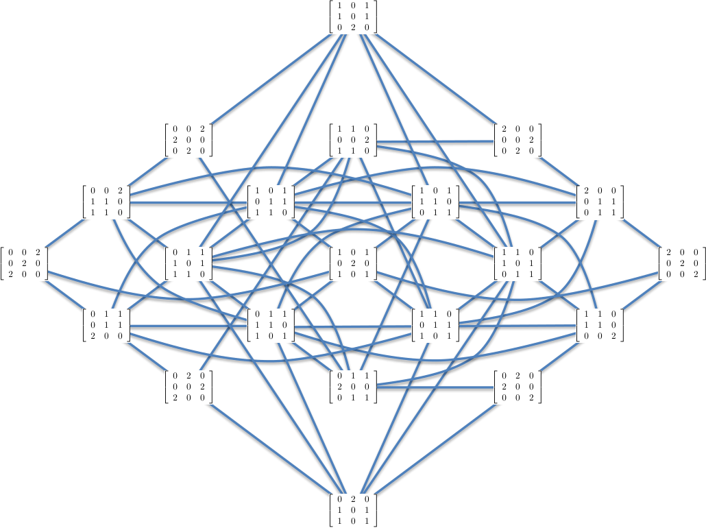
fig]fig:example
To state our main result, we need to mention some standard definitions from graph theory. The degree of a vertex in is the number of edges at . The minimum degree of a graph is the smallest of the degrees in the graph. A graph is -connected, , if and is connected for every set with . The connectivity of a graph is the largest such that is -connected.
The Metropolis-Hastings algorithm can be used for statistical tests for contingency tables. The algorithm performs a random walk on the fiber graph containing the contingency table we want to study [2]. The connectivity of the fiber graphs affects the convergence of the algorithm: typically, the lower the connectivity, the slower the convergence [6]. Our main result is:
Theorem 2.9.
The connectivity for .
We also prove several other statements regarding . The proof of the main result is based on Liu’s criterion [8], proved, for example, in [1]:
Lemma 2.8 (Liu’s criterion).
Let be a connected graph and . If for any two vertices and of with distance there are disjoint paths in , then is -connected.
For the first time, the following conjecture is confirmed for a large class of fiber graphs of an important and common class of Gröbner bases.
Conjecture (Engström ’12, [5][9]).
The connectivity of a large fiber graph of a reduced Gröbner basis of a lattice ideal is given by the minimum vertex degree of the fiber graph.
The technical version of the conjecture with the condition of a large fiber graph is spelled out in the appendix.
1.1 The basics of algebraic statistics
Let us review the basics of algebraic statistics. See the foundational paper [2] or the textbook [4] for an introduction to the field.
Fix an integer matrix whose column sums are equal. The probability simplex is . Let be the log-linear model associated with the matrix . The vector is the minimal sufficient statistic for and the fiber of a contingency table , represented in a vectorized form. Let ker be the integer kernel of the matrix . The finite set ker is a Markov basis for if there exists a sequence such that and for all ; all contingency tables and all pairs . The elements of the Markov basis are called Markov moves.
Another way of describing Markov bases is via finite subsets of lattices. In this case, we are interested in the integer lattice ker, where is the matrix associated with the log-linear model. The fiber of , for example, a contingency table in vectorized form, is the set , where is a lattice. Note that if ker, this definition is exactly the same as the definition of the fiber of a contingency table mentioned earlier. Let be an arbitrary finite subset of . The subset determines an undirected graph whose vertices are the elements of . Two vertices and are connected by an edge if either or is in . The subset is a Markov basis of if the graphs are connected for all . Fix a weight vector such that for all . The graph is an acyclic directed graph if the edges are now directed: , and present whenever is in . We call a Gröbner basis of if has a unique sink for all . Then, is called a fiber graph of a Gröbner basis. It is important to note that since our focus is on algebraic statistics and Markov bases, we undirect the edges of the fiber graphs of Gröbner bases and discuss ordinary connectivity instead of strong connectivity of directed graphs.
It is fruitful to view the previous notions from the standpoint of commutative algebra as well. A lattice can be represented by the lattice ideal . is a toric ideal. We can write with non-negative and for every . The following result is considered one of the starting points for algebraic statistics:
Theorem 1.1 (The fundamental theorem of Markov bases, [2]).
A subset of the lattice is a Markov basis if and only if the corresponding set of binomials generates the lattice ideal .
In the case of two-way contingency tables, the sufficient statistic is the row and columns sums of the tables and the matrix is chosen correspondingly. Since we consider the case of equal, fixed row and column sums, all tables are in the same fiber. The integer kernel of has a Markov basis whose cardinality is , namely , where denotes the matrix which has one in the position and zeroes elsewhere. This is exemplified in [2], and for an explicit proof of a more general result which implies it, see [4]. By Theorem 1.1, generates the lattice ideal . One can verify that the Markov basis gives a Gröbner basis by the cost vector with for the element on row and column . Since we need to have , the generators need to be of the form . The reason why the corresponding fiber graph has a unique sink is that the moves of this form are not possible from the anti-diagonal contingency table. The fact that this Gröbner basis is reduced is justified, for example, in Chapter 5 of [10]. As mentioned earlier, for the purposes of this paper, we undirect the edges of the fiber graph of the Gröbner basis. This means that the edges in our graph correspond exactly to the elements of the Markov basis , Markov moves.
1.2 Basic notation of graph theory
Next, we define a number of basic notions for graphs following those in [3]. Let be a graph, be the vertex set of and . The degree of a vertex in is the number of edges at . The minimum degree of a graph is the smallest of the degrees in the graph and the maximum degree the largest. We call a graph -connected, , if and is connected for every set with . The notation means a graph with the vertex set and edges of such that their endpoints are in . A subgraph of this type is called an induced subgraph of . By Menger’s Theorem [3, p. 71], a graph is -connected if and only if it contains independent (in other words, vertex-disjoint) paths between any two vertices. We will use disjoint as a synonym of independent. The connectivity of a graph is the largest such that is -connected, the distance between two vertices and of is the number of edges in a shortest path in , and the diameter diam of is defined as the largest distance in . The graph is -regular if, all its vertices have the same degree . If admits a partition into two classes such that the vertices in the same class are not adjacent, is called a bipartite graph. A matching in is a set of independent edges and it is called perfect if every vertex of is incident to exactly one edge in . A multigraph is a pair of disjoint sets together with a map that assigns two vertices to each edge. Here denotes the set of edges. A multigraph differs from an ordinary graph by allowing several edges between the same two vertices. As opposed to the definition in [3], our definition does not allow self-loops, edges that start from and end to the same vertex. The entry of the adjacency matrix of a multigraph is the number of edges from the vertex to the vertex . We define the biadjacency matrix of a bipartite multigraph as the submatrix of the adjacency matrix, where the columns correspond to the vertices in a bipartition class of the vertex set and rows to the vertices in the other class.
2 The fiber graphs
The first results are on the degree of the vertices of . The degree of is exactly the number of Markov moves that can be performed from . From here on, a move means a Markov move. Recall that here the set of Markov moves is the Markov basis
Thus, we want to calculate the number of unordered pairs
If we have such a pair, the entries and cannot be , and the move must then be possible from . We define the support of a vertex as the set
Note that the cardinality of is the number of positive entries in .
Lemma 2.1.
Let ,
- (a)
if has as its only positive entries, then .
- (b)
if does not have as its only positive entries, then .
Proof.
Part a). Since there are exactly nonzero entries in , all of them in different rows and columns, there are pairs . Thus, . To prove that is in this case the minimum degree, we need to prove part b) of this lemma.
Part b). Consider starting from a vertex that has as its only positive entries, and therefore support of size , and using a Markov move to get to . Now, because we must have , the size of the support must grow by at least two in the process. Therefore, the size of is at least . The pair can be picked in ways, because the row and column cannot contain any -entries if is positive, and there are other rows and columns which then need to contain positive entries. Hence, there are at least Markov moves from , and . ∎
Using the definition of connectivity with , being the vertex with all positive entries equal to , we get the following result as an immediate implication of Lemma 2.1.
Proposition 2.2.
The connectivity of satisfies .
Proposition 2.3.
If contains a vertex that has one as its only positive entries, then .
Proof.
If , we are done by Lemma 2.1 and the fact that all the vertices need to be of this type. Thus, assume . There has to be one-entries. Say that one of them is in the position . The row and column contain other one-entries. Therefore, there are pairs . All of these pairs correspond to a different Markov move from , and thus . Because the row and column sums are and we have an -matrix, for any . The equality corresponds to the case where the positive entries are all ones. Thus, if there is at least one >one-entry in , the number of positive entries is less than . Then, we can pick in less than ways. We claim that . If , we are done by Lemma 2.1. Let , and start from . Perform a Markov move from to so that an entry . If we would pick , the entry in the pair could be chosen in at most one more way than for the corresponding , because by our assumption, only can be both positive and such that its position, , is not in the support of . For any other , the number of pairs can only decrease or stay the same, since we can assume that and are in the support of but not in the support of . Moreover, since , and we assume that , if there is a positive entry of such that it is in the row but not in the column . If the pick is that entry, by our assumption there is one less possible pair for than a pair for the corresponding , because , but . On the other hand, if , the number of pairs where does not change while moving from to . As we iterate the process from , similar arguments hold. Thus, because we could pick in less than ways, and . Therefore, . ∎
Note that when , there is no such with all positive entries equal to one. Nevertheless, the maximum degree obtained is an upper bound for the vertex degree in that case as well. Thus, we know that . Now, having information on how the degree of the vertices of behaves, we try to find the connectivity . First, we will introduce a couple of auxiliary results:
Lemma 2.4.
The number of same Markov moves from with is at least for .
Proof.
Because and , . We want to know whether at least pairs of those positions are usable by a Markov move . Those positive entries in that are not in the support of must equal 1 or 2. Then, because , there has to be entries satisfying , at least one in the same column and one in the same row as such an entry. In general, each of the columns not containing an has to contain a positive entry as well. Having a positive entry in a particular column means that there cannot be an -entry in the same row. Thus, there is a positive entry not in this row in each of the other columns. We can choose a pair in total in ways by first selecting one of the columns and then one of the other columns. ∎
Theorem 2.5 (Kőnig, [7]).
Every -regular bipartite multigraph decomposes into perfect matchings.
Let be the -matrix with all entries 0, except for that position is 1.
Lemma 2.6.
Let be a vertex of and positions in an -matrix such that , and . Then there is a decomposition of into a sum of matrices that are vertices of such that for all .
Proof.
The proof is by induction on . For we are done. According to Theorem 2.5, every -regular bipartite multigraph decomposes into perfect matchings. Interpreting as the biadjacency matrix of an -regular bipartite multigraph, we get a decomposition into matrices with row and column sum 1. Assume that we have indexed the matrices such that . Let be a maximal subset of with 1, such that . By induction we can find a decomposition of admitting the conditions for | , and then we extend it. ∎
It might be of interest to the reader that the previous result, Lemma 2.6, implies that the semigroup generated by permutation matrices is a normal cone.
Proposition 2.7.
The graph is connected.
Proof.
The graph is the underlying undirected graph of a fiber graph of a Gröbner basis, and therefore connected. ∎
Lemma 2.8 (Liu’s criterion, [8]).
Let be a connected graph and . If for any two vertices and of with distance there are disjoint paths in , then is -connected.
A proof of Lemma 2.8 can be found in [1]. With these tools, we can set out to prove our main result:
Theorem 2.9.
The connectivity for .
Proof.
By Proposition 2.2, . Therefore, our goal is to show that is -connected. We aim to achieve this by applying Proposition 2.7 and Lemma 2.8 as well as a technique of building a large number of paths. We need to show that using the technique, we will in every case get at least independent paths. It turns out that the technique used will not work in the cases . If , . By Proposition 2.7, is connected and the case is done. Thus, we assume from now on that .
We will start by setting up the machinery. By Proposition 2.7, we can apply Lemma 2.8. Let with . Then there are Markov moves and such that . Because , does not correspond to a single move. Now, let us consider the sequences , where is an additional move, such that , as depicted in . Let be the number of ways to select so that we get disjoint paths. We want to show that is at least . Then we would have in total disjoint paths between and when we count the original path of length two as well. Note that the move has to be a valid Markov move from . By valid, we mean that the move does not take entries of negative (or correspondingly, larger than ). In other words, the move needs to connect to another vertex in the graph. The term possible move is used as a synonym for valid move.
fig]fig:idea
There are some remarks to be made:
- •
We must have , because would lead to an intersection. For the same reason, we need .
- •
If we can use or , we have . However, if both of them are valid Markov moves from , we have to subtract one from , because then the paths with and intersect.
- •
On the other hand, if the move is not valid, the path using does not connect and .
- •
If , the entries subtracts from are not usable by . By Lemma 2.1, in that case each of the vertices have the degree , and thus this method does not apply, because we will not get enough ways of choosing .
- •
If and cannot have even one same entry where they subtract from, again problematic in the cases where we start from a vertex with the degree . Then we cannot get the desired result using solely this procedure. For simplicity, assume .
The basic case.
Let us first assume that can subtract from the same entries as and . By this, we mean that the entries are large enough that we do not have to worry whether using before and causes an entry to be negative after performing or . Consider .
- •
We have at least ways of choosing such that , because d by Lemma 2.1.
- •
If it is even possible to select , some nonzero-entries of are not , and by Lemma 2.1, the degree of the vertex we are at is at least . Therefore, after subtracting the disallowed moves and , we have in this case, because .
However, we also have to take the case into account.
- •
If is possible, but , is not possible. Therefore, the previous results hold in this case as well.
- •
If also is possible as well as , by the earlier analysis we get , because with our assumption , .
- •
If on the other hand is not possible, we want to know whether the possibility is included in . If the number of entries of that prevent its use is at least two, must be , because will then subtract from entries zero in adds to. However, there is no point in this. Therefore, consider that has only one entry obstructing its use. Then subtracts from an entry zero in , which implies that has to add to that entry, but then would subtract from the entry. Thus, is not included in . If is to be possible, by Lemma 2.1, we need to be at with , because otherwise we would subtract from an -entry with , but then we would add to a zero-entry. Then . Otherwise we only need to avoid and have , because by Lemma 2.1.
Problematic entries.
Let us now move on to the cases where cannot subtract from all the entries where and . Then, the moves and subtract from entries smaller than two in . The number of this kind of problematic entries can range from one to four. By Lemma 2.4, the number of same Markov moves from and must be at least .
- •
First, say that subtracts from either four or three one-entries or two or one two-entry. Then the choices of moves at do not include or . We have to avoid , and thus .
- •
If and subtract from three one-entries in total, but the sum does not, there are six different cases: either or subtracts from two one-entries, and , or both add to an entry the other subtracts from. If subtracts from two one-entries, the moves and are clearly not possible at . Then we have . The same thing happens when subtracts from two one-entries and does not add to an entry subtracts from. In the two cases left, we cannot rely on Lemma 2.4.
- •
If and subtract from a total number of two one-entries, we either have the other one subtracting from two or both subtracting from one. In the latter case, if neither of them or only adds to an entry the other subtracts from, and are not possible at . Hence, in this case as well, we have .
The cases left are: only or subtracts from one-entries; subtracts from one one-entry, while subtracts from at least one different one-entry but adds to the one-entry subtracts from.
- •
If subtracts from one one-entry, where is the position of that particular one-entry. Following Lemma 2.6, decompose : , where and . The one-entry in the position in is now zero in . Because has one one-entry, it must have at least another. The second one-entry can either be in or . If it is in , , and if it is in , by Lemma 2.1. In the former case we get , where comes from the moves for and from the moves using the one entry not problematic in now in . In the latter case we have . We subtract two in both cases to avoid counting and .
- •
If subtracts from two one-entries at positions and , , and we decompose , where and . Thus, the problematic entries are zero in , and therefore also the move is not possible from . If , is not included in , and we have . Otherwise , and we get .
- •
If subtracts from one-entries some of which are also in , the case is treated exactly the same way as the two previous ones. If the particular one-entries are not in , cannot subtract from them and thus there is nothing to avoid.
- •
The case where subtracts from one one-entry and subtracts from one or two different one-entries, but adds to the one-entry subtracts from and at most one of the one-entries subtracts from is present in already, is treated exactly same way as the previous ones, because we have to avoid one or two problematic one-entries. If there are two problematic entries both already in , they can be avoided the same way as before. If there are three of them, all present in at positions , and , we have . Say that the two first are the ones used by . They can be put in the same in the proof of Lemma 2.6. Then we have , where . The problematic entries are zero in and the moves and are not possible from . Then only includes the disallowed choice . Thus .
Intersections.
The last question is what if different paths and intersect. By symmetry and straightforward calculations, the number of cases reduces to three: ; ; . The different types are drawn in :
fig]fig:intersections
The last case is the easiest to handle. Assume that we only have intersections of this type. An intersection can happen in two different ways.
- •
The moves and share one entry the other adds to and the other subtracts from. This sum can be written in three ways, one being the original, because and have to be Markov moves, both have to use three of the operations in and the cancelling operations can be done to three different entries. Therefore, this case amounts to two intersections. Let us a write an example to illustrate this:
- •
The other possibility, disjoint from the previous one, is that the positions of the non-zero rows or columns of and are the same. Then there are two ways, the original and another with swapped rows, to write the sum . This gives one intersection. Again, let us do a basic example:
To analyse how these affect the earlier calculations, we have to first note that the entries subtracts from must be at least two, because we want to subtract from the same entries with and . Only one of the two types is possible at a time.
- •
In the former case, there are two possibilities: either one or two intersections are possible. Let us first consider the case of one intersection. If (or if the order of the moves is switched) is to be included in , we must have , because there has to be at least three positive entries in one column, and therefore . The comes from three disallowed moves and one intersection. If not, the degree is at least by Lemma 2.1, which means we have . Now, assume that there are two intersections. The sum shows that there must be at least three positive entries in the -submatrix. However, when we write the sum in another way, the other move is . Thus, there has to be three additional positive entries, because in the different cases, subtracts in total from at least two of the one-entries in and one other entry. Hence, the support of has size at least . If we pick a positive entry from the -submatrix to be subtracted from by a Markov move, and the entry is such that four of the other five positive entries are on its row or column, the selection of the second positive entry can be done in ways, because there cannot be -entries in the row or column of the first entry. Clearly, if we pick the first entry in a different way, there are cases where the second selection can be done in even more ways, but no cases where in less. Thus, , because . The comes from three disallowed moves and two intersections.
- •
In the latter case, must be at least by Lemma 2.1, and we have , because we must have . We subtract four, because there are at most three disallowed moves and one intersection.
In the two other cases we have and sharing one non-zero row or column, which disappears in the sum . An example is presented below:
We assume that either or causes intersections, and denote the one causing them with . Let the other one be . Because and share one row with , also adds to a positive entry, because needs to subtract from that. Let the position of that entry be .
- •
Assume that at least one of the entries subtracts from satisfies . Then there must be at least one positive entry in the same column and one in the same row. If they are both in the row and column , is in the position . Otherwise, we can find 1-entries that do not use the row and the column for each subtracts from satisfying . Denote them with and . It might be that does not exist or . We have . They can all be put in the same in the construction of the proof of Lemma 2.6. Thus, by Lemma 2.6, we have , where is such that it does not contain the entries at most or subtract from. Because , and the choices and as well as intersections are avoided in , we have .
- •
Now, assume that both of the entries subtracts from are . As before, decompose using Lemma 2.6. This time, we cannot avoid the entries used by , but they will surely be large enough to be usable by . Again, does not contain the entries subtracted from by . Hence, we cannot have intersections of the other type occuring with moves from and have to only avoid , because adds to zero-entries, and thus is not included in . We have .
In the latter case, cannot cause intersections because of the assumption that subtracts from -entries, but in the former case it could. Because the entries subtracts from are in , the calculations hold even if intersections of the type are assumed possible. ∎
The last result in this paper concerns the diameter of :
Proposition 2.10.
The diameter of is .
Proof.
Every row sum is , and each of the positive entries can be selected to be subtracted from. Therefore, changes are enough to transform a row to any other. The :th row must be correct at least after changing the :th row, because otherwise we would have to change an already correct row to incorrect. The maximal number of changes needed is then , and diam.
Now, it suffices to show that diam. Take the diagonal matrix
The coordinates of the nonzero-entries are of the form . Consider permuting the rows so that , and . The result is
and the permutation matrix
On the other hand, . If is the number of operations needed to change to , the number of operations needed to change to is clearly .
Consider this procedure: start from the row . Find the row which has its one-entry in the column , in this case the second row, and swap the rows. Repeat this for each of the rows except for the :th one. Before the :th row is swapped for the second time, it will have its one-entry in the :th column, so by interchanging it with the :th row we will get to .
In our procedure, each of the swaps corrects the place of one one-entry except for the last one which corrects two. However, we might be able to use more swaps that correct two positions. These kind of interchanges require pairs of one-entries to be in positions of the form and . Say that we swap with to get and . Assume . If and , . Thus, the number of entries in a position of the form increases by at most one with each swap. There are positive entries in positions of the form in . To interchange the positions of two of entries (the entries not in the positions and some other) correcting both, we would then need at least one extra swap. Thus, the best possible result we could get this way is still swaps.
Each swap consists of one operation. Thus, , and therefore we need operations to make from . Hence, diam, but because also diam, diam. ∎
Appendix
In this appendix, we state the technical version of the conjecture mentioned in the introduction. The vertices of a fiber graph are the monomials in the preimage of some monomial in For some fixed lattice ideal and Gröbner basis, a fiber graph is -large if it is the preimage of a monomial that is divisible by For ideals from contingency tables this corresponds to that each row and column sum is at least
Conjecture (Engström ’12, [5][9]).
For any lattice ideal with a Gröbner basis, there is an such that the connectivity of any -large fiber graph is given by its minimum vertex degree.
This is an example by Raymond Hemmecke why the technical condition is needed. Construct a lattice ideal from the matrix
defining a map and use the Gröbner basis from lexicographic ordering. Then the fiber graph of the preimage of is the one dimensional skeleton of two -dimensional cubes connected by one edge. This fiber graph has minimum degree but is not 2-connected.
References
- [1] Anders Björner and Kathrin Vorwerk. Connectivity of chamber graphs of buildings and related complexes. European J. Combin. 31 (2010), no. 8, 2149–2160.
- [2] Persi Diaconis and Bernd Sturmfels. Algebraic algorithms for sampling from conditional distributions. Ann. Statist. 26 (1998), no. 1, 363–397.
- [3] Reinhard Diestel. Graph Theory. Fourth edition. Graduate Texts in Mathematics, 173. Springer, Heidelberg, 2010. 437 pp.
- [4] Mathias Drton, Bernd Sturmfels and Seth Sullivant. Lectures on Algebraic Statistics. Oberwolfach Seminars, Vol. 39. Birkhäuser, Basel, 2009. 172 pp.
- [5] Alexander Engström. Private communication, June 2012.
- [6] Shlomo Hoory, Nathan Linial and Avi Wigderson. Expander graphs and their applications. Bull. Amer. Math. Soc. (N.S.) 43 (2006), no. 4, 439–561
- [7] Dénes Kőnig. Über Graphen und ihre Anwendung auf Determinantentheorie und Mengenlehre. Math. Ann. 77 (1916), 453–465.
- [8] Gui Zhen Liu. Proof of a conjecture on matroid base graphs. Sci. China Ser. A 33 (1990), no. 11, 1329–1337.
- [9] Samu Potka. Connectivity, in "Problem book for Sannäs workshop, August 9-10, 2012", edited by Alexander Engström, 2012.
- [10] Bernd Sturmfels. Gröbner Bases and Convex Polytopes. University Lecture Series, Vol. 8. American Mathematical Society, Providence, R.I, 1996. 162 pp.
Samu Potka
Aalto University
Department of Mathematics and Systems Analysis
PO Box 11100
FI-00076 Aalto
Finland
e-mail: samu.potka@aalto.fi