跳到论文正文
W Papers独立论文阅读器 arXiv:1209.1525 论文正文 计算阅读时间 · 0%
引用这篇论文根据当前论文元数据生成,正式投稿前建议核对。


License: arXiv.org perpetual non-exclusive license
arXiv:1209.1525v2 [hep-ph] 14 Sep 2012

UAB-FT 722

On the S-wave pollution of B→K∗​l+​l−B\to K^{*}l^{+}l^{-} observables

Joaquim Matias
Universitat Autònoma de Barcelona, 08193 Bellaterra, Barcelona, Spain

The angular distribution B→K∗(→Kπ)l+l−B\to K^{*}(\to K\pi)l^{+}l^{-} is nowadays, but also in the near future, one of the central players in our search for New Physics in rare B decays. A wide variety of experimental analysis have been presented [1, 2, 3, 4] focusing on different observables related to this rich mode. Simultaneously, there has been a huge effort from the theory community to provide a complete and accurate description of this 4-body decay mode [5]-[16]. Given the relevance of this mode in providing new constraints [17]-[28] it is of utmost importance to control and isolate any possible source of hadronic pollution that can spoil a clear signal of the theory that lies beyond the SM.

In a recent interesting paper [16] one possible source of pollution of the angular distribution B→K∗(→Kπ)l+l−B\to K^{*}(\to K\pi)l^{+}l^{-} due to events coming from the distribution B→K0∗(→Kπ)l+l−B\to K_{0}^{*}(\to K\pi)l^{+}l^{-}, where K0∗K_{0}^{*} is a scalar meson resonance, was analyzed. There it was presented the full distribution of the combined channels B→K∗(→Kπ)l+l−B\to K^{*}(\to K\pi)l^{+}l^{-} and B→K0∗(→Kπ)l+l−B\to K_{0}^{*}(\to K\pi)l^{+}l^{-} and the focus was on the impact that this pollution could have on the extraction of the transverse asymmetries AT(2)A_{T}^{(2)} [6], AT(re)A_{T}^{({\rm re})}[14] and AT(im)A_{T}^{({\rm im})}[14]. In [16] it was argued that even if one should expect that the transverse asymmetries are unaffected by this S-wave contamination, they are afflicted from this disease via their normalization. They conclude that if the transverse asymmetries (defined with an unusual normalization) are measured in the particular way they propose, they are afflicted by this pollution at the level of less than 10%\% in all q2q^{2}-range except for q2=2q^{2}=2 GeV2 where the pollution can be as large as 23%23\%.

In this short note we present a simple procedure to bypass this pollution and extract the transverse asymmetries defined as in [15] in a way completely free from any S-wave contamination including also all lepton mass corrections. First, we show using folded distributions, that an exact (mℓ≠0m_{\ell}\neq 0) and clean (no S-wave pollution) extraction of all the PiP_{i} observables [15] is perfectly possible. Second, we argue that even using uniangular distributions a strategy can be designed to reduce the impact of the companion decay on the transverse asymmetries to only lepton mass suppressed terms. Incidentally, we also present two procedures to introduce lepton mass corrections inside the observables in the distribution, an exact one preserving the structure of the massless case as much as possible and an approximated one that minimizes the error of neglecting lepton masses. The results presented here aim at reducing substantially two main sources of systematic errors of the experimental data namely the S-wave pollution and lepton mass corrections. The final goal is to provide strategies to enhance the sensitivity to any possible signal of New Physics affecting the clean observables P1,2,3P_{1,2,3}, P4,5,6′P_{4,5,6}^{\prime}.

In Section I we recall the definitions of the known observables, introduce new ones and we also present a so called “massless-improved limit”. In Section II we show how to extract the PiP_{i} observables in an exact way using folded distributions including all lepton mass corrections with zero S-wave pollution. Also a less clean approximate procedure is discussed using uniangular distributions. In appendices A and B we define the coefficients of the distribution coming from the companion scalar decay B→K0∗(→Kπ)l+l−B\to K_{0}^{*}(\to K\pi)l^{+}l^{-} and provide more examples of folded distributions.

Abstract

It has been argued recently that transverse asymmetries that are expected to be shielded from the presence of the S-wave K​πK\pi pairs originating from the decay of a scalar K0∗K_{0}^{*} meson, are indeed affected by this pollution due to the impossibility to extract cleanly the normalization for these observables. In this short note we show how using folded distributions, which is nowadays the preferred method to obtain the information from the 4-body decay mode B→K∗(→Kπ)l+l−B\to K^{*}(\to K\pi)l^{+}l^{-}, one can easily bypass this problem and extract the clean observables P1,2,3P_{1,2,3} and also P4,5,6′P_{4,5,6}^{\prime} in a way completely free from this pollution including all lepton mass corrections. We also show that in case one insists in using uniangular distributions to extract these observables it is possible to reduce this pollution to just lepton mass suppressed terms. On the contrary, the SiS_{i} observables, that are by definition normalized by the full differential decay distribution, will indeed suffer from this pollution via their normalization. Finally, we also present a procedure to minimize the error associated to neglecting lepton mass corrections in the distribution defining a massless-improved limit.

I. Definitions: Observables, full distribution and massless-improved limit

The angular distribution that describes the four-body decay B→K∗(→Kπ)l+l−B\to K^{*}(\to K\pi)l^{+}l^{-} including the S-wave pollution from the companion decay B→K0∗(→Kπ)l+l−B\to K_{0}^{*}(\to K\pi)l^{+}l^{-} is [6, 9, 16]

d4​Γdq2dcosθKdcosθldϕ\displaystyle\frac{d^{4}\Gamma}{dq^{2}\,d\!\cos\theta_{K}\,d\!\cos\theta_{l}\,d\phi} =\displaystyle= 932​π[J1​ssin2θK+J1​ccos2θK+(J2​ssin2θK+J2​ccos2θK)cos2θl\displaystyle\frac{9}{32\pi}\bigg[J_{1s}\sin^{2}\theta_{K}+J_{1c}\cos^{2}\theta_{K}+(J_{2s}\sin^{2}\theta_{K}+J_{2c}\cos^{2}\theta_{K})\cos 2\theta_{l} (1)
+J3sin2θKsin2θlcos2ϕ+J4sin2θKsin2θlcosϕ+J5sin2θKsinθlcosϕ\displaystyle\hskip-76.82234pt+J_{3}\sin^{2}\theta_{K}\sin^{2}\theta_{l}\cos 2\phi+J_{4}\sin 2\theta_{K}\sin 2\theta_{l}\cos\phi+J_{5}\sin 2\theta_{K}\sin\theta_{l}\cos\phi
+(J6​ssin2θK+J6​ccos2θK)cosθl+J7sin2θKsinθlsinϕ+J8sin2θKsin2θlsinϕ\displaystyle\hskip-76.82234pt+(J_{6s}\sin^{2}\theta_{K}+{J_{6c}\cos^{2}\theta_{K}})\cos\theta_{l}+J_{7}\sin 2\theta_{K}\sin\theta_{l}\sin\phi+J_{8}\sin 2\theta_{K}\sin 2\theta_{l}\sin\phi
+J9sin2θKsin2θlsin2ϕ]X+S\displaystyle\hskip-76.82234pt+J_{9}\sin^{2}\theta_{K}\sin^{2}\theta_{l}\sin 2\phi\bigg]\,X+S

where

S\displaystyle S =\displaystyle= 14​π[J~1​ac+J~1​bccosθK+(J~2​ac+J~2​bccosθK)cos2θℓ+J~4sinθKsin2θℓcosϕ\displaystyle\frac{1}{4\pi}\left[{\tilde{J}}_{1a}^{c}+{\tilde{J}}_{1b}^{c}\cos\theta_{K}+({\tilde{J}}_{2a}^{c}+{\tilde{J}}_{2b}^{c}\cos\theta_{K})\cos 2\theta_{\ell}+{\tilde{J}}_{4}\sin\theta_{K}\sin 2\theta_{\ell}\cos\phi\right. (2)
+J~5sinθKsinθℓcosϕ+J~7sinθKsinθℓsinϕ+J~8sinθKsin2θℓsinϕ]\displaystyle\left.+{\tilde{J}}_{5}\sin\theta_{K}\sin\theta_{\ell}\cos\phi+{\tilde{J}}_{7}\sin\theta_{K}\sin\theta_{\ell}\sin\phi+{\tilde{J}}_{8}\sin\theta_{K}\sin 2\theta_{\ell}\sin\phi\right]

and

X=∫d​mK​π2​|B​WK∗​(mK​π2)|2\displaystyle X=\int dm_{K\pi}^{2}|BW_{K^{*}}(m_{K\pi}^{2})|^{2} (3)

being a correction introduced in [16] to take into account the width of the resonance (see [16] for precise definition and details on this function). This correction factorizes from the standard JiJ_{i} defined in [6, 7, 9] and as, we will show, it will always cancel in the PiP_{i} observables. The J~i{\tilde{J}}_{i} containing the interference terms coming from the B→K0∗(→Kπ)l+l−B\to K^{*}_{0}(\to K\pi)l^{+}l^{-} decay computed in [16] are defined in Appendix A.

The full differential decay distribution is then

d​Γf​u​l​ld​q2=d​ΓK∗d​q2+d​ΓK0∗d​q2\displaystyle\frac{d\Gamma_{full}}{dq^{2}}=\frac{d\Gamma_{K^{*}}}{dq^{2}}+\frac{d\Gamma_{K_{0}^{*}}}{dq^{2}} (4)

with

d​ΓK∗d​q2=14​(3​J1​c+6​J1​s−J2​c−2​J2​s)​X,d​ΓK0∗d​q2=+2​J~1​ac−23​J~2​ac\displaystyle\frac{d\Gamma_{K^{*}}}{dq^{2}}=\frac{1}{4}\left(3J_{1c}+6J_{1s}-J_{2c}-2J_{2s}\right)X,\quad\frac{d\Gamma_{K_{0}^{*}}}{dq^{2}}=+2{\tilde{J}}_{1a}^{c}-\frac{2}{3}{\tilde{J}}_{2a}^{c} (5)

Here we will not consider scalar contributions to facilitate the comparison with [16] where they were also neglected. Notice that the distribution including lepton masses (but neglecting scalars J6c=0J_{6}^{c}=0) contains 11 JiJ_{i} coefficients (only 10 are independent [10, 15]) plus 8 J~i{\tilde{J}}_{i} coefficients coming from the interference with the S-wave polluting process. A generalization of the results presented here to include scalars is straightforward. We take the same inputs as in [28] and all observables should be understood as J→J+J¯J\to J+{\bar{J}} (obviously the same applies for expressions written in terms of transversity amplitudes).

The first important point is the exact definition of the transverse asymmetries in terms of the coefficients of the distribution. In [16] the transverse asymmetries are defined with an unusual normalization

A~T(2)=4​J3​(q2)3​J1​s​(q2)−J2​s​(q2)\displaystyle{{\tilde{A}}_{T}^{(2)}}={4J_{3}(q^{2})\over 3J_{1s}(q^{2})-J_{2s}(q^{2})} ,AT(im)(q2)=4​J9​(q2)3​J1​s​(q2)−J2​s​(q2),\displaystyle\,,\quad A_{T}^{({\rm im})}(q^{2})={4J_{9}(q^{2})\over 3J_{1s}(q^{2})-J_{2s}(q^{2})}\,,
AT(re)​(q2)=\displaystyle A_{T}^{({\rm re})}(q^{2})= βℓ​J6​s​(q2)3​J1​s​(q2)−J2​s​(q2).\displaystyle{\beta_{\ell}J_{6s}(q^{2})\over 3J_{1s}(q^{2})-J_{2s}(q^{2})}\,.\quad (6)

This choice of normalization in [16] is driven by the aim of extracting it from the θK\theta_{K} uniangular distribution (see below). These definitions albeit correct have two main disadvantages:

  • •

    The expression of the transverse asymmetries given in Eq.(6) once expressed in terms of transversity amplitudes involves lepton mass terms via the coefficient11 1 From now on we will distinguish between two types of lepton mass dependences: lepton mass terms that will refer to terms like the last term in Eq.(7) and mass dependence via the prefactor βℓ\beta_{\ell}.

    J1​s\displaystyle J_{1s} =\displaystyle= (2+βℓ2)4​[|A⟂L|2+|A∥L|2+|A⟂R|2+|A∥R|2]+4​mℓ2q2​Re​(A⟂L​A⟂R∗+A∥L​A∥R∗)\displaystyle\frac{(2+\beta_{\ell}^{2})}{4}\left[|{A_{\perp}^{L}}|^{2}+|{A_{\|}^{L}}|^{2}+|{A_{\perp}^{R}}|^{2}+|{A_{\|}^{R}}|^{2}\right]+\frac{4m_{\ell}^{2}}{q^{2}}{\rm Re}\left({A_{\perp}^{L}}{A_{\perp}^{R}}^{*}+{A_{\|}^{L}}{A_{\|}^{R}}^{*}\right)\, (7)

    where βℓ=1−4​mℓ2/q2\beta_{\ell}=\sqrt{1-4m_{\ell}^{2}/q^{2}}. This implies that their definition is not invariant under changes of the lepton mass (ℓ=e,μ\ell=e,\mu).

  • •

    Normalization requires to measure two coefficients of the distribution.

For these two reasons we prefer to stick to the definition of the PiP_{i} observables as given in [15]. These definitions in terms of transversity amplitudes do not dependent on any lepton mass term:

P1\displaystyle P_{1} =\displaystyle= |A⟂L|2−|A∥L|2+(L↔R)|A⟂L|2+|A∥L|2+(L↔R)=J32​J2​s,\displaystyle\frac{|A_{\perp}^{L}|^{2}-|A_{\|}^{L}|^{2}+(L\leftrightarrow R)}{|A_{\perp}^{L}|^{2}+|A_{\|}^{L}|^{2}+(L\leftrightarrow R)}=\frac{J_{3}}{2J_{2s}}\ ,\
P2\displaystyle P_{2} =\displaystyle= Re(A⟂L∗A∥L−A⟂RA∥R∗)|A⟂L|2+|A∥L|2+(L↔R)=βℓ​J6​s8​J2​s,\displaystyle\frac{{\rm Re}(A_{\perp}^{L*}A_{\|}^{L}-A_{\perp}^{R}A_{\|}^{R*})}{|A_{\perp}^{L}|^{2}+|A_{\|}^{L}|^{2}+(L\leftrightarrow R)}=\beta_{\ell}\frac{J_{6s}}{8J_{2s}}\ ,\ \quad
P3\displaystyle P_{3} =\displaystyle= Im(A⟂L∗A∥L−A⟂RA∥R∗)|A⟂L|2+|A∥L|2+(L↔R)=−J94​J2​s\displaystyle\frac{{\rm Im}(A_{\perp}^{L*}A_{\|}^{L}-A_{\perp}^{R}A_{\|}^{R*})}{|A_{\perp}^{L}|^{2}+|A_{\|}^{L}|^{2}+(L\leftrightarrow R)}=-\frac{J_{9}}{4J_{2s}} (8)

These observables were completed in [28] with

P4′\displaystyle P_{4}^{\prime} =\displaystyle= 2Re(A0L∗A∥L+A0RA∥R∗)(|A⟂L|2+|A∥L|2+(L↔R))​(|A0L|2+(L↔R))=J4−J2​c​J2​s,\displaystyle\frac{\sqrt{2}{\rm Re}(A_{0}^{L*}A_{\|}^{L}+A_{0}^{R}A_{\|}^{R*})}{\sqrt{\left(|A_{\perp}^{L}|^{2}+|A_{\|}^{L}|^{2}+(L\leftrightarrow R)\right)\left(|A_{0}^{L}|^{2}+(L\leftrightarrow R)\right)}}=\frac{J_{4}}{\sqrt{-J_{2c}J_{2s}}}\ ,\ \quad
P5′\displaystyle P_{5}^{\prime} =\displaystyle= 2Re(A0L∗A⟂L−A0RA⟂R∗)(|A⟂L|2+|A∥L|2+(L↔R))​(|A0L|2+(L↔R))=βℓ2​J5−J2​c​J2​s,\displaystyle\frac{\sqrt{2}{\rm Re}(A_{0}^{L*}A_{\perp}^{L}-A_{0}^{R}A_{\perp}^{R*})}{\sqrt{\left(|A_{\perp}^{L}|^{2}+|A_{\|}^{L}|^{2}+(L\leftrightarrow R)\right)\left(|A_{0}^{L}|^{2}+(L\leftrightarrow R)\right)}}=\frac{\beta_{\ell}}{2}\frac{J_{5}}{\sqrt{-J_{2c}J_{2s}}}\ ,\ \quad
P6′\displaystyle P_{6}^{\prime} =\displaystyle= 2Im(A0L∗A∥L+A0RA∥R∗)(|A⟂L|2+|A∥L|2+(L↔R))​(|A0L|2+(L↔R))=−βℓ2​J7−J2​c​J2​s\displaystyle\frac{\sqrt{2}{\rm Im}(A_{0}^{L*}A_{\|}^{L}+A_{0}^{R}A_{\|}^{R*})}{\sqrt{\left(|A_{\perp}^{L}|^{2}+|A_{\|}^{L}|^{2}+(L\leftrightarrow R)\right)\left(|A_{0}^{L}|^{2}+(L\leftrightarrow R)\right)}}=-\frac{\beta_{\ell}}{2}\frac{J_{7}}{\sqrt{-J_{2c}J_{2s}}}\ (9)

where the βℓ\beta_{\ell} prefactor included in P2,5′,6′P_{2,5^{\prime},6^{\prime}} is there to ensure that the expression in terms of transversity amplitudes does not contain any lepton mass dependence. P1P_{1} is the transverse asymmetry AT(2)A_{T}^{(2)} proposed in [6] and P2P_{2} and P3P_{3} correspond to the AT(re)A_{T}^{({\rm re})} and AT(im)A_{T}^{({\rm im})}, respectively, normalized as in [14] and not like in Eq.(6). Notice also that the normalization of the transverse asymmetries in Eqs.(8) requires to measure one single coefficient of the distribution, namely, J2​sJ_{2s}, free from any lepton mass term.

It is very convenient to express the coefficients of the angular distribution directly in terms of observables. In Ref. [15] it was presented the most complete expression of the coefficients of the distribution including lepton masses and scalars in terms of the full basis of observables. Later on, in [28] a very compact parametrization was found for the massless case without scalar contributions. Here we present a generalization of Ref. [28] to include lepton masses with a similar structure to the massless case at the price of trading the original basis [15]

{d​ΓK∗d​q2,AFB,P1,2,3,P4,5,6,M1,M2}→{F^T​d​ΓK∗d​q2,F^L​d​ΓK∗d​q2,F~T​d​ΓK∗d​q2,F~L​d​ΓK∗d​q2,P1,2,3,P4,5,6′}\Big\{\frac{d\Gamma_{K^{*}}}{dq^{2}},A_{\rm FB},P_{1,2,3},P_{4,5,6},M_{1},M_{2}\Big\}\to\Big\{{\hat{F}}_{T}\frac{d\Gamma_{K^{*}}}{dq^{2}},{\hat{F}}_{L}\frac{d\Gamma_{K^{*}}}{dq^{2}},{\tilde{F}}_{T}\frac{d\Gamma_{K^{*}}}{dq^{2}},{\tilde{F}}_{L}\frac{d\Gamma_{K^{*}}}{dq^{2}},P_{1,2,3},P_{4,5,6}^{\prime}\Big\}

The exact parametrization of the coefficients in the massive case is then22 2 Notice that in the first coefficient J1​sJ_{1s} the βℓ\beta_{\ell} dependence does not appear explicitly (but it is included inside F^T{\hat{F}}_{T}). The reason is that parametrized in this way and only in this coefficient the mass dependence piece of βℓ\beta_{\ell} will help later on to reduce the contribution from the lepton mass term.

J1​s\displaystyle J_{1s} =34​F^T​1X​d​ΓK∗d​q2,\displaystyle=\dfrac{3}{4}{\hat{F}}_{T}\frac{1}{X}\frac{d\Gamma_{K^{*}}}{dq^{2}}, J2​s=14​βℓ2​F~T​1X​d​ΓK∗d​q2,\displaystyle J_{2s}=\dfrac{1}{4}\beta_{\ell}^{2}{\tilde{F}}_{T}\frac{1}{X}\frac{d\Gamma_{K^{*}}}{dq^{2}},
J1​c\displaystyle J_{1c} =F^L​1X​d​ΓK∗d​q2,\displaystyle={\hat{F}}_{L}\frac{1}{X}\frac{d\Gamma_{K^{*}}}{dq^{2}}\ , J2​c=−βℓ2​F~L​1X​d​ΓK∗d​q2,\displaystyle J_{2c}=-\beta_{\ell}^{2}{\tilde{F}}_{L}\frac{1}{X}\frac{d\Gamma_{K^{*}}}{dq^{2}}\ ,
J3\displaystyle J_{3} =12​βℓ2​P1​F~T​1X​d​ΓK∗d​q2,\displaystyle=\dfrac{1}{2}\beta_{\ell}^{2}P_{1}{\tilde{F}}_{T}\frac{1}{X}\frac{d\Gamma_{K^{*}}}{dq^{2}}, J6​s=2​βℓ​P2​F~T​1X​d​ΓK∗d​q2,\displaystyle J_{6s}=2\beta_{\ell}P_{2}{\tilde{F}}_{T}\frac{1}{X}\frac{d\Gamma_{K^{*}}}{dq^{2}},
J4\displaystyle J_{4} =12​βℓ2​P4′​F~T​F~L​1X​d​ΓK∗d​q2,\displaystyle=\dfrac{1}{2}\beta_{\ell}^{2}{P_{4}^{\prime}}\sqrt{{\tilde{F}}_{T}{\tilde{F}}_{L}}\ \frac{1}{X}\frac{d\Gamma_{K^{*}}}{dq^{2}}, J9=−βℓ2​P3​F~T​1X​d​ΓK∗d​q2,\displaystyle J_{9}=-\beta_{\ell}^{2}P_{3}{\tilde{F}}_{T}\frac{1}{X}\frac{d\Gamma_{K^{*}}}{dq^{2}}\ ,
J5\displaystyle J_{5} =βℓ​P5′​F~T​F~L​1X​d​ΓK∗d​q2,\displaystyle=\beta_{\ell}P_{5}^{\prime}\sqrt{{\tilde{F}}_{T}{\tilde{F}}_{L}}\ \frac{1}{X}\frac{d\Gamma_{K^{*}}}{dq^{2}}\ ,
J7\displaystyle J_{7} =−βℓ​P6′​F~T​F~L​1X​d​ΓK∗d​q2,\displaystyle=-\beta_{\ell}P_{6}^{\prime}\sqrt{{\tilde{F}}_{T}{\tilde{F}}_{L}}\ \frac{1}{X}\frac{d\Gamma_{K^{*}}}{dq^{2}}\ , (10)

and the redundant but interesting coefficient J8J_{8} is

J8=−12​βℓ2​Q′​F~T​F~L​1X​d​ΓK∗d​q2\displaystyle J_{8}=-\frac{1}{2}\beta_{\ell}^{2}Q^{\prime}\sqrt{{\tilde{F}}_{T}{\tilde{F}}_{L}}\ \frac{1}{X}\frac{d\Gamma_{K^{*}}}{dq^{2}} (11)

where the new observables F^T,L{\hat{F}}_{T,L}, F~T,L{\tilde{F}}_{T,L} are given by

F^T\displaystyle{\hat{F}}_{T} =\displaystyle= 163​N​[(2+βℓ2)4​[|A⟂L|2+|A∥L|2+|A⟂R|2+|A∥R|2]+4​mℓ2q2​Re​(A⟂L​A⟂R∗+A∥L​A∥R∗)]=16​J1​s3​N\displaystyle\frac{16}{3N}\left[\frac{(2+\beta_{\ell}^{2})}{4}\left[|{A_{\perp}^{L}}|^{2}+|{A_{\|}^{L}}|^{2}+|{A_{\perp}^{R}}|^{2}+|{A_{\|}^{R}}|^{2}\right]+\frac{4m_{\ell}^{2}}{q^{2}}{\rm Re}\left({A_{\perp}^{L}}{A_{\perp}^{R}}^{*}+{A_{\|}^{L}}{A_{\|}^{R}}^{*}\right)\right]=\frac{16J_{1s}}{3N}
F^L\displaystyle{\hat{F}}_{L} =\displaystyle= 4N​[|A0L|2+|A0R|2+4​mℓ2q2​[|At|2+2​R​e​(A0L​A0R∗)]]=4​J1​cN\displaystyle\frac{4}{N}\left[|{A_{0}^{L}}|^{2}+|{A_{0}^{R}}|^{2}+\frac{4m_{\ell}^{2}}{q^{2}}\left[|A_{t}|^{2}+2{\rm Re}({A_{0}^{L}}{A_{0}^{R}}^{*})\right]\right]=\frac{4J_{1c}}{N}
F~T\displaystyle{\tilde{F}}_{T} =\displaystyle= 4N​[|A⟂L|2+|A∥L|2+|A⟂R|2+|A∥R|2]=16​J2​sβℓ2​N\displaystyle\frac{4}{N}\left[|{A_{\perp}^{L}}|^{2}+|{A_{\|}^{L}}|^{2}+|{A_{\perp}^{R}}|^{2}+|{A_{\|}^{R}}|^{2}\right]=\frac{16J_{2s}}{\beta_{\ell}^{2}N}
F~L\displaystyle{\tilde{F}}_{L} =\displaystyle= 4N​[|A0L|2+|A0R|2]=−4​J2​cβℓ2​N\displaystyle\frac{4}{N}\left[|{A_{0}^{L}}|^{2}+|{A_{0}^{R}}|^{2}\right]=-\frac{4J_{2c}}{\beta_{\ell}^{2}N} (12)

and the normalization is

N\displaystyle N =\displaystyle= [(3+βℓ2)(|A⟂L|2+|A∥L|2+|A0L|2+|A⟂R|2+|A∥R|2+|A0R|2)+\displaystyle\left[(3+\beta_{\ell}^{2})\left(|{A_{\perp}^{L}}|^{2}+|{A_{\|}^{L}}|^{2}+|{A_{0}^{L}}|^{2}+|{A_{\perp}^{R}}|^{2}+|{A_{\|}^{R}}|^{2}+|{A_{0}^{R}}|^{2}\right)+\right.
+12​mℓ2q2[|At|2+2Re(A0LA0R∗+A⟂LA⟂R∗+A∥LA∥R∗)]]=3J1​c+6J1​s−J2​c−2J2​s=4Xd​ΓK∗d​q2.\displaystyle\left.+\frac{12m_{\ell}^{2}}{q^{2}}\left[|A_{t}|^{2}+2{\rm Re}({A_{0}^{L}}{A_{0}^{R}}^{*}+{A_{\perp}^{L}}{A_{\perp}^{R}}^{*}+{A_{\|}^{L}}{A_{\|}^{R}}^{*})\right]\right]=3J_{1c}+6J_{1s}-J_{2c}-2J_{2s}=\frac{4}{X}\frac{d\Gamma_{K^{*}}}{dq^{2}}.

At this point several remarks are in order:

  • I.

    PiP_{i} and Pj′P_{j}^{\prime} q2q^{2}-dependent observables once expressed in terms of transversity amplitudes do not dependent on mℓm_{\ell}, on the contrary F^T,L{\hat{F}}_{T,L} and F~T,L{\tilde{F}}_{T,L} do depend.

  • II.

    Eqs.(10) and Eq.(11) are exact concerning lepton masses (no scalars included). In all the folded distributions discussed in next section we will always use this exact parametrization.

  • III.

    They are constructed to resemble Eqs.(14) of [28] for the massless case. The main difference with the massless case is that here there are two longitudinal polarization fractions and two transverse polarization fractions and the sums of transverse and longitudinal fractions differ slightly from one:

    F^L+F^T=1+δ^F~T+F~L=1+δ{\hat{F}}_{L}+{\hat{F}}_{T}=1+{\hat{\delta}}\quad\quad{\tilde{F}}_{T}+{\tilde{F}}_{L}=1+\delta

    In the exact massless limit F^L|mℓ=0=F~L|mℓ=0{\hat{F}}_{L}|_{m_{\ell}=0}={\tilde{F}}_{L}|_{m_{\ell}=0}, F^T|mℓ=0=F~T|mℓ=0{\hat{F}}_{T}|_{m_{\ell}=0}={\tilde{F}}_{T}|_{m_{\ell}=0} and δ^,δ→0{\hat{\delta}},\delta\to 0. A numerical expression for δ⁡(s)\delta(s) is provided in Table 1. δ^​(s){\hat{\delta}}(s) will be re-expressed in terms of other quantities below.

  • IV.

    The βℓ\beta_{\ell} dependence in the coefficients is kept explicit (except for J1​sJ_{1s}). This choice will be fundamental when approaching the massless limit to reduce the systematic associated to this limit.
Refer to caption
Refer to caption
Refer to caption
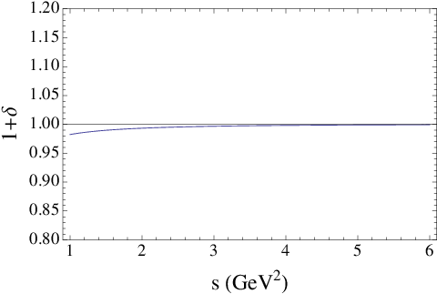
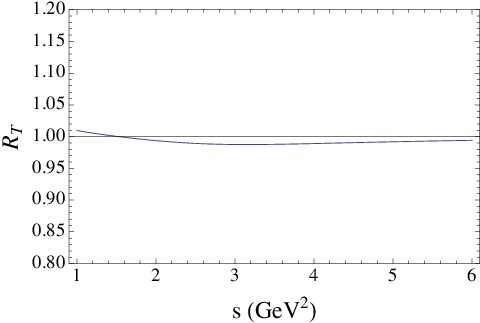
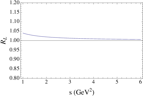
Figure 1: (left) ratio RT=F^T/F~TR_{T}={\hat{F}}_{T}/{\tilde{F}}_{T} always below 1.2%1.2\% in SM, (middle) ratio RL=F^L/F~LR_{L}={\hat{F}}_{L}/{\tilde{F}}_{L} with an error range between 1%1\% to less than 4%4\% in the SM (right) δ\delta represents the deviation from one of F~L\tilde{F}_{L}+F~T\tilde{F}_{T}.

We will explore now in a bit more of detail the massless limit. It is clear that in the exact massive case one should strictly fit the data to four observables F^L,T{\hat{F}}_{L,T}, F~L,T{\tilde{F}}_{L,T} apart from the six clean PiP_{i}. The ratios RT≡F^T/F~TR_{T}\equiv{\hat{F}}_{T}/{\tilde{F}}_{T} and RL≡F^L/F~LR_{L}\equiv{\hat{F}}_{L}/{\tilde{F}}_{L} are indeed a direct measurement of the clean observables M1M_{1} and M2M_{2} defined in [15]:

RT=13​(2+(1+4​M1)​βℓ2)RL=1+M2R_{T}=\frac{1}{3}\left(2+(1+4M_{1})\beta_{\ell}^{2}\right)\quad\quad R_{L}=1+M_{2}

The deviation from one of these ratios in the SM in the range 11 to 66 GeV2 are shown in Fig.1. They are below 1.2%1.2\% for RTR_{T} and below 4%4\% for RLR_{L}. Moreover, given the tight relation of these ratios with M1,2M_{1,2} and the relatively small deviations found in these observables in the New Physics scenarios analyzed in [15], a similar range of deviations is expected also for New Physics.

Finally, since it is very costly in statistics to fit for the four observables F^T,L{\hat{F}}_{T,L}, F~T,L{\tilde{F}}_{T,L} one could take the massless limit (mℓ→0m_{\ell}\to 0 everywhere) to reduce the number of observables to fit. However, the exact massless limit could induce errors of order 4%4\% (around q2=1q^{2}=1 GeV2) for instance if F^L=F~L{\hat{F}}_{L}={\tilde{F}}_{L} is used (see RLR_{L} in Fig.1). For this reason we prefer to define an intermediate limit, that we call “massless-improved limit”. This consists in keeping the βℓ\beta_{\ell} dependence of Eqs.(10) and reexpressing F^T{\hat{F}}_{T} and F^L{\hat{F}}_{L} in terms of F~T{\tilde{F}}_{T} in the following way

F^T\displaystyle{\hat{F}}_{T} =\displaystyle= F~T+(RT−1)​F~T≡F~T+L1\displaystyle{\tilde{F}}_{T}+(R_{T}-1){\tilde{F}}_{T}\equiv{\tilde{F}}_{T}+L_{1} (13)
F^L\displaystyle{\hat{F}}_{L} =\displaystyle= 1−F~T+δ+(RL−1)​(1−F~T)+𝒪⁡((RL−1)​δ)≡1−F~T+L2\displaystyle 1-{\tilde{F}}_{T}+{\delta}+(R_{L}-1)(1-{\tilde{F}}_{T})+{\cal O}((R_{L}-1){\delta})\equiv 1-{\tilde{F}}_{T}+L_{2} (14)

where 𝒪⁡((RL−1)​δ){\cal O}((R_{L}-1){\delta}) is much below the permille level and δ^​(s)=L1+L2{\hat{\delta}}(s)=L_{1}+L_{2}. A numerical expression for L1,2L_{1,2} in the SM can be found in Table 1. In this improved limit the contribution to F^L,T{\hat{F}}_{L,T} from lepton mass terms (L1,L2L_{1},L_{2}) in the SM is always below 1.3%1.3\% in all q2q^{2}-region from 1 to 6 GeV2. Notice that the PiP_{i} are not directly affected by this limit since they are always defined by the same F~T,L{\tilde{F}}_{T,L}, but they are only indirectly affected via the propagation of the error in the determination of F~T,L{\tilde{F}}_{T,L}. The reason for the sizeable reduction from 4%4\% to near 1.3%1.3\% in the case of F^L{\hat{F}}_{L} is due to the partial cancellation between δ\delta and (RL−1)​(1−F~T)(R_{L}-1)(1-{\tilde{F}}_{T}) in the SM (see Fig.1). This means that the error done by expressing the coefficients of the exact angular distribution Eqs.(10) and Eq.(11) only in terms of F~T,L{\tilde{F}}_{T,L} (keeping the βℓ\beta_{\ell} dependence but discarding the L1,2L_{1,2} corrections) is below 1.3%1.3\%.

Concerning the integrated observables there are two important observations when including lepton masses. First notice that

F~T​d​ΓK∗d​q2=(F~T​d​ΓK∗d​q2)|mℓ=0{\tilde{F}}_{T}\frac{d\Gamma_{K^{*}}}{dq^{2}}=\left({\tilde{F}}_{T}{\frac{d\Gamma_{K^{*}}}{dq^{2}}}\right)\Bigl|_{m_{\ell}=0}

and

F~T​F~L​d​ΓK∗d​q2=(F~T​F~L​d​ΓK∗d​q2)|mℓ=0\sqrt{{\tilde{F}}_{T}{\tilde{F}}_{L}}\frac{d\Gamma_{K^{*}}}{dq^{2}}=\left(\sqrt{{\tilde{F}}_{T}{\tilde{F}}_{L}}{\frac{d\Gamma_{K^{*}}}{dq^{2}}}\right)\Bigl|_{m_{\ell}=0}

which means that these products are the same for the massive and massless case. Second important remark is that three of the q2q^{2}-dependent PiP_{i} observables include a βℓ\beta_{\ell} in their expression in terms of the JiJ_{i} coefficients and this can be problematic when defining integrated observables. The reason being that what is measured are the JiJ_{i} coefficients and not products like βℓ​Ji\beta_{\ell}J_{i}. Consequently, a small redefinition of three of these observables is required when including lepton masses in the integrated observables. This means that the integrated observables in the massive case naturally split in two categories:

  • •

    First set: P1P_{1}, P3P_{3} and P4′P_{4}^{\prime} their q2q^{2}-expression in terms of spin amplitudes and JiJ_{i} coefficients do not contain neither lepton mass terms nor βℓ\beta_{\ell} prefactors.

    <P1mℓ≠0>b​i​n\displaystyle<P_{1}^{m_{\ell}\neq 0}>_{bin} =\displaystyle= ∫b​i​nJ32​∫b​i​nJ2​s=∫b​i​nβℓ2​P1​F~T​dΓK∗d​q2∫b​i​nβℓ2​F~T​dΓK∗d​q2\displaystyle\frac{\int_{bin}J_{3}}{2\int_{bin}J_{2s}}=\frac{\int_{bin}\beta_{\ell}^{2}P_{1}{\tilde{F}}_{T}\frac{d\Gamma_{K*}}{dq^{2}}}{\int_{bin}\beta_{\ell}^{2}{\tilde{F}}_{T}\frac{d\Gamma_{K*}}{dq^{2}}}
    <P3mℓ≠0>b​i​n\displaystyle<P_{3}^{m_{\ell}\neq 0}>_{bin} =\displaystyle= −∫b​i​nJ94​∫b​i​nJ2​s=∫b​i​nβℓ2​P3​F~T​dΓK∗d​q2∫b​i​nβℓ2​F~T​dΓK∗d​q2\displaystyle-\frac{\int_{bin}J_{9}}{4\int_{bin}J_{2s}}=\frac{\int_{bin}\beta_{\ell}^{2}P_{3}{\tilde{F}}_{T}\frac{d\Gamma_{K*}}{dq^{2}}}{\int_{bin}\beta_{\ell}^{2}{\tilde{F}}_{T}\frac{d\Gamma_{K*}}{dq^{2}}}
    <P4′mℓ≠0>b​i​n\displaystyle<P_{4}^{\prime\,m_{\ell}\neq 0}>_{bin} =\displaystyle= ∫b​i​nJ4−∫b​i​nJ2​c∫b​i​nJ2​s=∫b​i​nβℓ2​P4′​F~T​F~L​dΓK∗d​q2∫b​i​nβℓ2​F~T​dΓK∗d​q2​∫b​i​nβℓ2​F~L​dΓK∗d​q2.\displaystyle\frac{\int_{bin}J_{4}}{\sqrt{-\int_{bin}J_{2c}\int_{bin}J_{2s}}}=\frac{\int_{bin}\beta_{\ell}^{2}P_{4}^{\prime}\,\sqrt{{\tilde{F}}_{T}{\tilde{F}}_{L}}\frac{d\Gamma_{K*}}{dq^{2}}}{\sqrt{\int_{bin}\beta_{\ell}^{2}{\tilde{F}}_{T}\frac{d\Gamma_{K*}}{dq^{2}}\int_{bin}\beta_{\ell}^{2}{\tilde{F}}_{L}\frac{d\Gamma_{K*}}{dq^{2}}}}. (15)

    For these observables P1mℓ≠0=P1P_{1}^{m_{\ell}\neq 0}=P_{1}, P3mℓ≠0=P3P_{3}^{m_{\ell}\neq 0}=P_{3} and P4′mℓ≠0=P4′P_{4}^{\prime\,m_{\ell}\neq 0}=P_{4}^{\prime}. Naturally, only when expressing them directly in terms of observables the βℓ\beta_{\ell} prefactor arises.

  • •

    Second set: P2P_{2}, P5′P_{5}^{\prime}, P6′P_{6}^{\prime} also their q2q^{2}-expression in terms of spin amplitudes do not contain any lepton mass terms or βℓ\beta_{\ell} prefactors. However their q2−q^{2}-differential expression in terms of JiJ_{i} do contain a βℓ\beta_{\ell} prefactor, which means that its corresponding massive definition for the integrated observables requires a redefinition with a prefactor 1/βℓ1/\beta_{\ell}:

    <P2mℓ≠0>b​i​n\displaystyle<P_{2}^{m_{\ell}\neq 0}>_{bin} =\displaystyle= ∫b​i​nJ6​s8​∫b​i​nJ2​s=∫b​i​nβℓ2​(P2/βℓ)​F~T​dΓK∗d​q2∫b​i​nβℓ2​F~T​dΓK∗d​q2\displaystyle\frac{\int_{bin}J_{6s}}{8\int_{bin}J_{2s}}=\frac{\int_{bin}\beta_{\ell}^{2}(P_{2}/\beta_{\ell}){\tilde{F}}_{T}\frac{d\Gamma_{K*}}{dq^{2}}}{\int_{bin}\beta_{\ell}^{2}{\tilde{F}}_{T}\frac{d\Gamma_{K*}}{dq^{2}}}
    <P5′mℓ≠0>b​i​n\displaystyle<P_{5}^{\prime\,m_{\ell}\neq 0}>_{bin} =\displaystyle= ∫b​i​nJ52​−∫b​i​nJ2​c∫b​i​nJ2​s=∫b​i​nβℓ2​(P5′/βℓ)​F~T​F~L​dΓK∗d​q2∫b​i​nβℓ2​F~T​dΓK∗d​q2​∫b​i​nβℓ2​F~L​dΓK∗d​q2\displaystyle\frac{\int_{bin}J_{5}}{2\sqrt{-\int_{bin}J_{2c}\int_{bin}J_{2s}}}=\frac{\int_{bin}\beta_{\ell}^{2}(P_{5}^{\prime}/\beta_{\ell})\sqrt{{\tilde{F}}_{T}{\tilde{F}}_{L}}\frac{d\Gamma_{K*}}{dq^{2}}}{\sqrt{\int_{bin}\beta_{\ell}^{2}{\tilde{F}}_{T}\frac{d\Gamma_{K*}}{dq^{2}}\int_{bin}\beta_{\ell}^{2}{\tilde{F}}_{L}\frac{d\Gamma_{K*}}{dq^{2}}}}
    <P6′mℓ≠0>b​i​n\displaystyle<P_{6}^{\prime\,m_{\ell}\neq 0}>_{bin} =\displaystyle= −∫b​i​nJ72​−∫b​i​nJ2​c∫b​i​nJ2​s=∫b​i​nβℓ2​(P6′/βℓ)​F~T​F~L​dΓK∗d​q2∫b​i​nβℓ2​F~T​dΓK∗d​q2​∫b​i​nβℓ2​F~L​dΓK∗d​q2\displaystyle-\frac{\int_{bin}J_{7}}{2\sqrt{-\int_{bin}J_{2c}\int_{bin}J_{2s}}}=\frac{\int_{bin}\beta_{\ell}^{2}(P_{6}^{\prime}/\beta_{\ell})\sqrt{{\tilde{F}}_{T}{\tilde{F}}_{L}}\frac{d\Gamma_{K*}}{dq^{2}}}{\sqrt{\int_{bin}\beta_{\ell}^{2}{\tilde{F}}_{T}\frac{d\Gamma_{K*}}{dq^{2}}\int_{bin}\beta_{\ell}^{2}{\tilde{F}}_{L}\frac{d\Gamma_{K*}}{dq^{2}}}} (16)

    where P2mℓ≠0=P2/βℓP_{2}^{m_{\ell}\neq 0}=P_{2}/\beta_{\ell}, P5′mℓ≠0=P5′/βℓP_{5}^{\prime\,m_{\ell}\neq 0}=P_{5}^{\prime}/\beta_{\ell} and P6′mℓ≠0=P6′/βℓP_{6}^{\prime\,m_{\ell}\neq 0}=P_{6}^{\prime}/\beta_{\ell}.

The last important point here is to compare the SM predictions for the massive integrated observables defined here <Pimℓ≠0><P_{i}^{m_{\ell}\neq 0}> with the massless ones computed in [28]. We will focus the comparison on the 1-bin region between 1 to 6 GeV2. For the first set due to the balance of βℓ2\beta_{\ell}^{2} factors between numerator and denominator of Eqs.(15) together with the slow variation of this factor with ss, one should expect a tiny difference between the massive and the massless prediction. Indeed we found that the massive prediction in the SM is only +0.8%+0.8\% larger than the massless one for P1P_{1} and P4′P_{4}^{\prime} and below permille level for P3P_{3}. In the second set the comparison of the SM integrated observable in the range 1 to 6 GeV2 in the massless and massive case is −0.6%-0.6\%, +1.4%+1.4\% and +0.8%+0.8\% for P2P_{2}, P5′P_{5}^{\prime} and P6′P_{6}^{\prime} respectively. This implies that the massless predictions in the SM obtained in [28] are valid to an excellent approximation also in the massive case.

11 ss s2s^{2} s3s^{3} s4s^{4} s5s^{5}
i 00 11 22 33 44 55
dim GeV0 GeV-2 GeV-4 GeV-6 GeV-8 GeV-10
δi\delta_{i} -0.0498563 +0.0502874 -0.0228207 +0.00540332 -0.000644906 +0.000030558
RT​iR_{T\,i} +1.02522 -0.0074101 -0.0142605 +0.00717305 -0.00120443 +0.0000692328
RL​iR_{L\,i} +1.09905 -0.09191 +0.041595 -0.00990168 +0.00118789 -0.0000565414
L1​iL_{1\,i} +0.0201856 -0.0273282 +0.0135174 -0.00331905 +0.000403496 -0.0000193199
L2​iL_{2\,i} -0.00598948 +0.0255013 -0.0149247 +0.00389817 -0.000488089 +0.0000237576
Table 1: Coefficients of the polynomial approximation to the deviation parameters δ\delta, RTR_{T}, RLR_{L}, L1L_{1} and L2L_{2}, such that δ=∑i=0,5δi​si\delta=\sum_{i=0,5}\delta_{i}s^{i}, RT=∑i=0,5RT​i​siR_{T}=\sum_{i=0,5}R_{T\,i}s^{i}, RL=∑i=0,5RL​i​siR_{L}=\sum_{i=0,5}R_{L\,i}s^{i}, L1=∑i=0,5L1​i​siL_{1}=\sum_{i=0,5}L_{1\,i}s^{i} and L2=∑i=0,5L2​i​siL_{2}=\sum_{i=0,5}L_{2\,i}s^{i}.

In conclusion in this section we have proposed to use either the exact parametrization or an approximate parametrization so called ”massless-improved” limit for the experimental fit (instead of the pure massless limit). This improved parametrization has the advantage of including the dominant contribution from lepton masses with an error when compared to the exact result that amounts only to a maximum of a 1.3%1.3\% in the SM for the terms that contained F^L,T{\hat{F}}_{L,T} in the region between 1 to 6 GeV2 while it is exact for the q2q^{2} -dependent PiP_{i} observables (up to the propagation of the error in the determination of F~T,L{\tilde{F}}_{T,L}). The practical consequence of this improved limit is to effectively reduce the basis of observables to one observable less {d​ΓK∗d​q2,F~T,F~L,P1,2,3,P4,5,6′}\{\frac{d\Gamma_{K^{*}}}{dq^{2}},{\tilde{F}}_{T},{\tilde{F}}_{L},P_{1,2,3},P_{4,5,6}^{\prime}\} (since we are taking M1→0M_{1}\to 0). If one neglects in addition δ\delta (keeping the βℓ\beta_{\ell} dependence) by using F~L∼1−F~T{\tilde{F}}_{L}\sim 1-{\tilde{F}}_{T} an additional error associated to this second approximation (see Fig.1) should be added. In this case the previous basis gets reduced to eight observables. This step by step procedure will help to know precisely the size of the error associated to each approximation. Once this is done, next step is to compare with the theory predictions. We have shown here that the comparison of the exact massive predictions in the SM with the massless predictions [28] in the 1 to 6 GeV2 bin for the integrated observables shows a deviation that in the worst case amounts to 1.4%1.4\%.

II. Can one extract the observables P1,2,3P_{1,2,3} and P4,5,6′P_{4,5,6}^{\prime} free from S-wave pollution?

In order to answer this question two aspects have to be analyzed. On the one hand, the intrinsic character of the observable with respect to the S-wave pollution and, on the other, the extraction procedure of the observable.

Concerning the first aspect, one should distinguish the observables that does not suffer from S-wave pollution by construction from those that have an inherent structure that includes the pollution. It is clear that the products

F~T​d​ΓK∗d​q2,F~L​d​ΓK∗d​q2,Pi​F~T​d​ΓK∗d​q2Pj′​F~L​F~T​d​ΓK∗d​q2{\tilde{F}}_{T}\frac{d\Gamma_{K^{*}}}{dq^{2}},\quad{\tilde{F}}_{L}\frac{d\Gamma_{K^{*}}}{dq^{2}},\quad P_{i}{\tilde{F}}_{T}\frac{d\Gamma_{K^{*}}}{dq^{2}}\quad P_{j}^{\prime}\sqrt{{\tilde{F}}_{L}{\tilde{F}}_{T}}\frac{d\Gamma_{K^{*}}}{dq^{2}}

but also PiP_{i}, Pj′P_{j}^{\prime} with i=1,2,3i=1,2,3 and j=4,5,6j=4,5,6 are all intrinsically free from this contamination. Notice that these products enter in the definition of integrated observables. Consequently the corresponding integrated observables are also intrinsically free from S-wave pollution.

On the contrary, for instance, the SiS_{i} observables [9] are normalized by the full differential decay distribution

Si=Ji+J¯id​Γf​u​l​ld​q2\displaystyle S_{i}=\frac{J_{i}+{\bar{J}}_{i}}{\frac{d\Gamma_{full}}{dq^{2}}} (17)

and they will be directly affected by the S-wave pollution given that the full differential decay distribution is largely affected by this disease (see Eq.(5)). Any other observable normalized by d​Γf​u​l​ld​q2\frac{d\Gamma_{full}}{dq^{2}}, like for example a longitudinal polarization fraction normalized by the full distribution (call it F¯L{\bar{F}}_{L}), will be strongly S-wave polluted, however the product F¯L​d​Γf​u​l​ld​q2{\bar{F}}_{L}\frac{d\Gamma_{full}}{dq^{2}} is again free from pollution.

Concerning the extraction procedure, in the following we will show that it is possible to extract these observables completely free from any S-wave pollution in the exact lepton mass case and, afterwards, we will present for completeness also an approximate solution using uniangular distributions.

Exact solution including lepton mass corrections using folded distributions

The crucial point here is to determine the exact procedure to extract the PiP_{i} observables. There are basically two choices: uniangular distributions or the full angular distribution. The major drawback of the former is that by integrating angles the distinct angular dependence of the unwanted J~i{\tilde{J}}_{i} is lost and mixing (and pollution) with the interesting JiJ_{i} is unavoidable. If, instead, the full angular distribution is used the major problem is that there is not yet enough statistics to have access to the full distribution. However, the clever idea presented in Ref.[4] of using “folded” distributions, have the double advantage of increasing the statistics and focusing on a restricted set of angular coefficients. This allows to extract information from this mode in a more selective way than traditional uniangular distributions and, in particular, it can be used, as we will show, to isolate the polluting J~i{\tilde{J}_{i}} terms. In this note we will exploit this trick to show that using folded distributions one can measure all PiP_{i} and Pj′P_{j}^{\prime} free from any S-wave pollution thanks to their distinct angular dependence.

In Ref. [4], the identification of ϕ↔ϕ+π\phi\leftrightarrow\phi+\pi (when ϕ<0\phi<0) has been used to produce a “folded” angle ϕ^∈[0,π]\hat{\phi}\in[0,\pi] in terms of which a (folded) differential decay rate d​Γ^=d​Γ​(ϕ^)+d​Γ​(ϕ^−π)d\hat{\Gamma}=d\Gamma(\hat{\phi})+d\Gamma(\hat{\phi}-\pi) is obtained33 3 Other examples of singled folded distributions exhibiting dependencies on P1,2,3P_{1,2,3} but with the angle θK\theta_{K} instead can be found in Appendix B.. This folding exploits the angular symmetries of the distribution and reduce to a subset the coefficients entering each folded distribution. If we use the same folding procedure including the extra terms coming from the pollution channel B→K0∗(→Kπ)l+l−B\to K_{0}^{*}(\to K\pi)l^{+}l^{-} one finds the well known structure for the angular distribution together with an extra piece with a distinguishable angular dependence

d4​Γ^dq2dcosθKdcosθldϕ^\displaystyle\frac{d^{4}\hat{\Gamma}}{dq^{2}\,d\!\cos\theta_{K}\,d\!\cos\theta_{l}\,d\hat{\phi}} =\displaystyle= 916​π[J1​ccos2θK+J1​s(1−cos2θK)+J2​ccos2θK(2cos2θℓ−1)\displaystyle\frac{9}{16\pi}\bigg[{J_{1c}}\cos^{2}{\theta_{K}}+{J_{1s}}(1-\cos^{2}{\theta_{K}})+{J_{2c}}\cos^{2}{\theta_{K}}(2\cos^{2}{\theta_{\ell}}-1) (18)
+J2​s​(1−cos2⁡θK)​(2​cos2⁡θℓ−1)+J3​(1−cos2⁡θK)​(1−cos2⁡θℓ)​cos⁡2​ϕ^\displaystyle\hskip-42.67912pt+{J_{2s}}(1-\cos^{2}{\theta_{K}})(2\cos^{2}{\theta_{\ell}}-1)+{J_{3}}(1-\cos^{2}{\theta_{K}})(1-\cos^{2}{\theta_{\ell}})\cos{2\hat{\phi}}
+J6​s(1−cos2θK)cosθℓ+J9(1−cos2θK)(1−cos2θℓ)sin2ϕ^]X+W1\displaystyle\hskip-42.67912pt+{J_{6s}}(1-\cos^{2}{\theta_{K}})\cos{\theta_{\ell}}+{J_{9}}(1-\cos^{2}{\theta_{K}})(1-\cos^{2}{\theta_{\ell}})\sin{2\hat{\phi}}\bigg]X+W_{1}

where

W1=12​π[J~1​ac+J~1​bccosθK+(J~2​ac+J~2​bccosθK)(2cos2θℓ−1)]\displaystyle W_{1}=\frac{1}{2\pi}\left[{\tilde{J}}_{1a}^{c}+{\tilde{J}}_{1b}^{c}\cos\theta_{K}+\left({\tilde{J}}_{2a}^{c}+{\tilde{J}}_{2b}^{c}\cos\theta_{K}\right)(2\cos^{2}{\theta_{\ell}}-1)\right] (19)

The extra factor W1W_{1} concentrates all the S-wave pollution of this folded distribution. Its distinct angular dependence can be parametrized by

W1=aW+bW(2cos2θℓ−1)+cWcosθK+dWcosθK(2cos2θℓ−1)\displaystyle W_{1}=a_{W}+b_{W}(2\cos^{2}\theta_{\ell}-1)+c_{W}\cos\theta_{K}+d_{W}\cos\theta_{K}(2\cos^{2}\theta_{\ell}-1) (20)

Fitting for these four parameters (aW,bW,cW,dWa_{W},b_{W},c_{W},d_{W}) one can measure and disentangle the S-wave pollution.44 4 Notice that if lepton mass suppressed terms from the polluting decay B→K0∗​l​lB\to K_{0}^{*}ll are disregarded aW=−bWa_{W}=-b_{W} and cW=−dWc_{W}=-d_{W} But, more importantly, the different angular dependence associated to the relevant coefficients involved in the definition of the P1,2,3P_{1,2,3} permits an extraction of these observables in a way completely free from any S-wave pollution. It is clear from the definition of P1,2,3P_{1,2,3} in Eq.(8) that the folded distribution provides access to J3J_{3}, J6​sJ_{6s} and J9J_{9}, numerators of P1P_{1}, P2P_{2} and P3P_{3} respectively. But also their common denominator J2​sJ_{2s} is identified with the coefficient of (1−cos2⁡θK)​(2​cos2⁡θℓ−1)(1-\cos^{2}\theta_{K})(2\cos^{2}\theta_{\ell}-1). The normalization of A~T2{\tilde{A}_{T}}^{2}, AT(re)A_{T}^{({\rm re})} and AT(im)A_{T}^{({\rm im})} presented in [16] requires to measure in addition J1​cJ_{1c}, unnecessary for the P1,2,3P_{1,2,3}.

This is more easily seen writing down Eq.(18) in terms of observables using Eqs.(10). The following expression generalizes Eq.(1) of the LHCb note [4] by including lepton mass corrections and the S-wave pollution in a compact form:

d4​Γ^dq2dcosθKdcosθldϕ^\displaystyle\frac{d^{4}\hat{\Gamma}}{dq^{2}\,d\!\cos\theta_{K}\,d\!\cos\theta_{l}\,d\hat{\phi}} =\displaystyle= 916​π[F^Lcos2θK+34F^T(1−cos2θK)−βℓ2F~Lcos2θK(2cos2θℓ−1)\displaystyle\frac{9}{16\pi}\bigg[{\hat{F}_{L}}\cos^{2}{\theta_{K}}+\frac{3}{4}{\hat{F}_{T}}(1-\cos^{2}{\theta_{K}})-\beta_{\ell}^{2}{\tilde{F}_{L}}\cos^{2}{\theta_{K}}(2\cos^{2}{\theta_{\ell}}-1) (21)
+14​βℓ2​F~T​(1−cos2⁡θK)​(2​cos2⁡θℓ−1)+12​βℓ2​P1​F~T​(1−cos2⁡θK)​(1−cos2⁡θℓ)​cos⁡2​ϕ^\displaystyle\hskip-105.2751pt+\frac{1}{4}\beta_{\ell}^{2}{\tilde{F}}_{T}(1-\cos^{2}{\theta_{K}})(2\cos^{2}{\theta_{\ell}}-1)+\frac{1}{2}\beta_{\ell}^{2}P_{1}{\tilde{F}}_{T}(1-\cos^{2}{\theta_{K}})(1-\cos^{2}{\theta_{\ell}})\cos{2\hat{\phi}}
+2βℓP2F~T(1−cos2θK)cosθℓ−βℓ2P3F~T(1−cos2θK)(1−cos2θℓ)sin2ϕ^]dΓK∗d​q2+W1\displaystyle\hskip-105.2751pt+2\beta_{\ell}P_{2}{\tilde{F}}_{T}(1-\cos^{2}{\theta_{K}})\cos{\theta_{\ell}}-\beta_{\ell}^{2}P_{3}{\tilde{F}}_{T}(1-\cos^{2}{\theta_{K}})(1-\cos^{2}{\theta_{\ell}})\sin{2\hat{\phi}}\bigg]\,\frac{d\Gamma_{K*}}{dq^{2}}+W_{1}

or in the massless-improved limit:

d4​Γ^dq2dcosθKdcosθldϕ^\displaystyle\frac{d^{4}\hat{\Gamma}}{dq^{2}\,d\!\cos\theta_{K}\,d\!\cos\theta_{l}\,d\hat{\phi}} =\displaystyle= 916​π[(1−F~T)cos2θK+34F~T(1−cos2θK)−βℓ2F~Lcos2θK(2cos2θℓ−1)\displaystyle\frac{9}{16\pi}\bigg[(1-{\tilde{F}_{T}})\cos^{2}{\theta_{K}}+\frac{3}{4}{\tilde{F}_{T}}(1-\cos^{2}{\theta_{K}})-\beta_{\ell}^{2}{\tilde{F}_{L}}\cos^{2}{\theta_{K}}(2\cos^{2}{\theta_{\ell}}-1) (22)
+14​βℓ2​F~T​(1−cos2⁡θK)​(2​cos2⁡θℓ−1)+12​βℓ2​P1​F~T​(1−cos2⁡θK)​(1−cos2⁡θℓ)​cos⁡2​ϕ^\displaystyle\hskip-91.04872pt+\frac{1}{4}\beta_{\ell}^{2}{\tilde{F}}_{T}(1-\cos^{2}{\theta_{K}})(2\cos^{2}{\theta_{\ell}}-1)+\frac{1}{2}\beta_{\ell}^{2}P_{1}{\tilde{F}}_{T}(1-\cos^{2}{\theta_{K}})(1-\cos^{2}{\theta_{\ell}})\cos{2\hat{\phi}}
+2βℓP2F~T(1−cos2θK)cosθℓ−βℓ2P3F~T(1−cos2θK)(1−cos2θℓ)sin2ϕ^]dΓK∗d​q2+W1\displaystyle\hskip-91.04872pt+2\beta_{\ell}P_{2}{\tilde{F}}_{T}(1-\cos^{2}{\theta_{K}})\cos{\theta_{\ell}}-\beta_{\ell}^{2}P_{3}{\tilde{F}}_{T}(1-\cos^{2}{\theta_{K}})(1-\cos^{2}{\theta_{\ell}})\sin{2\hat{\phi}}\bigg]\,\frac{d\Gamma_{K*}}{dq^{2}}+W_{1}\,

where the βℓ\beta_{\ell} dependence is kept, F^L{\hat{F}}_{L} is traded by F~T{\tilde{F}}_{T} and the L1,2L_{1,2} subleading terms have been dropped off. The error of this improved limit is below 1.3%1.3\% as discussed in the previous section.

There is also an alternative that can be automatically applied to all the folded distributions discussed here and it is to use d​Γf​u​l​ld​q2\frac{d\Gamma_{full}}{dq^{2}} instead of dΓK∗d​q2\frac{d\Gamma_{K*}}{dq^{2}}, i.e,

d4​Γ^dq2dcosθKdcosθldϕ^\displaystyle\frac{d^{4}\hat{\Gamma}}{dq^{2}\,d\!\cos\theta_{K}\,d\!\cos\theta_{l}\,d\hat{\phi}} =\displaystyle= 916​π[F^¯Lcos2θK+34F^¯T(1−cos2θK)−βℓ2F~¯Lcos2θK(2cos2θℓ−1)\displaystyle\frac{9}{16\pi}\bigg[{\bar{\hat{F}}_{L}}\cos^{2}{\theta_{K}}+\frac{3}{4}{\bar{\hat{F}}_{T}}(1-\cos^{2}{\theta_{K}})-\beta_{\ell}^{2}{\bar{\tilde{F}}_{L}}\cos^{2}{\theta_{K}}(2\cos^{2}{\theta_{\ell}}-1) (23)
+14​βℓ2​F~¯T​(1−cos2⁡θK)​(2​cos2⁡θℓ−1)+12​βℓ2​P1​F~¯T​(1−cos2⁡θK)​(1−cos2⁡θℓ)​cos⁡2​ϕ^\displaystyle\hskip-105.2751pt+\frac{1}{4}\beta_{\ell}^{2}{\bar{\tilde{F}}_{T}}(1-\cos^{2}{\theta_{K}})(2\cos^{2}{\theta_{\ell}}-1)+\frac{1}{2}\beta_{\ell}^{2}P_{1}{\bar{\tilde{F}}_{T}}(1-\cos^{2}{\theta_{K}})(1-\cos^{2}{\theta_{\ell}})\cos{2\hat{\phi}}
+2βℓP2F~¯T(1−cos2θK)cosθℓ−βℓ2P3F~¯T(1−cos2θK)(1−cos2θℓ)sin2ϕ^]d​Γf​u​l​ld​q2+W1\displaystyle\hskip-105.2751pt+2\beta_{\ell}P_{2}{\bar{\tilde{F}}_{T}}(1-\cos^{2}{\theta_{K}})\cos{\theta_{\ell}}-\beta_{\ell}^{2}P_{3}{\bar{\tilde{F}}_{T}}(1-\cos^{2}{\theta_{K}})(1-\cos^{2}{\theta_{\ell}})\sin{2\hat{\phi}}\bigg]\,\frac{d\Gamma_{full}}{dq^{2}}+W_{1}

where all quantities with a bar are defined by Y¯=C​Y\bar{Y}=CY with

C=dΓK∗d​q2d​Γf​u​l​ld​q2C=\frac{\frac{d\Gamma_{K*}}{dq^{2}}}{\frac{d\Gamma_{full}}{dq^{2}}}

Notice that, as explained in the previous section, no S-wave pollution is introduced in this way in the relevant q2q^{2} or integrated PiP_{i} observables. Here the improved-massless limit becomes defined by

F^¯T=C​F^T\displaystyle{\bar{\hat{F}}_{T}}=C{\hat{F}}_{T} =\displaystyle= C​F~T+(RT−1)​C​F~T=C​F~T+C​L1\displaystyle C{\tilde{F}}_{T}+(R_{T}-1)C{\tilde{F}}_{T}=C{\tilde{F}}_{T}+CL_{1} (24)

where the relative error induced by dropping C​L1CL_{1} in C​F~TC{{\tilde{F}}_{T}} is obviously the same as before, below 1.2%1.2\%. However for F^¯L{\bar{\hat{F}}_{L}} two possibilities are now open depending on the size of CC. First possibility, if |C−1||C-1| is comparable in size to C​L2CL_{2} taking into account that C−1C-1 is negative while C​L2CL_{2} is positive a partial cancellation can take place and the best approach is to use

F^¯L=C​F^L\displaystyle{\bar{\hat{F}}_{L}}=C{\hat{F}}_{L} =\displaystyle= 1−C​F~T+C​L2+(C−1)\displaystyle 1-C{\tilde{F}}_{T}+CL_{2}+(C-1) (25)

In practice this require |C−1||C-1| to be below 4%4\% to be a good choice (given that L2L_{2} is below 1%1\%). The second possibility is to take

F^¯L=C​F^L\displaystyle{\bar{\hat{F}}_{L}}=C{\hat{F}}_{L} =\displaystyle= C​F~L+(RL−1)​C​F~L\displaystyle C{\tilde{F}}_{L}+(R_{L}-1)C{\tilde{F}}_{L} (26)

In this case the relative error RL−1R_{L}-1 is independent of CC exactly as for F^¯R{\bar{\hat{F}}_{R}}, however it rises up to 4%4\% at q2=1q^{2}=1 GeV2 as can be seen in Fig. 1. This choice is safer because the error does not depend on CC but the high remaining error (4%4\%) implies that the advantage of the massless-improved limit in front of the massless case is lost.

At this point it is evident the power of this folding technique, in the massive case the full distribution would depend on 11 JiJ_{i} coefficients (only 10 of them are independent) plus 8 J~i{\tilde{J}}_{i} coefficients from the companion decay. Instead, the folded distribution depends only on seven JiJ_{i} coefficients (or seven observables F^T,F^L,F~T,F~L,P1,P2,P3{\hat{F}}_{T},{\hat{F}}_{L},{\tilde{F}}_{T},{\tilde{F}}_{L},P_{1},P_{2},P_{3} ) and four J~i{\tilde{J}}_{i} (aW,bW,cW,dWa_{W},b_{W},c_{W},d_{W}). If the improved-massless limit is used the number of observables reduces to six: d​ΓK∗/d​q2,F~Td\Gamma_{K^{*}}/{dq^{2}},{\tilde{F}}_{T}, F~L{\tilde{F}}_{L}, P1P_{1}, P2P_{2}, P3P_{3} plus the four from J~i{\tilde{J}}_{i}.

Notice also that the prefactor X=∫d​mK​π2​|B​WK∗​(mK​π2)|2X=\int dm_{K\pi}^{2}|BW_{K^{*}}(m_{K\pi}^{2})|^{2} cancels out exactly in the PiP_{i} given their definition in terms of ratios of coefficients.

One can also exploit further this technique and find several doubled-folded distribution showing different dependencies on the P1,2,3P_{1,2,3} observables and exhibiting common/different S-wave pollutions. For instance, two possible foldings of the angles ϕ\phi and θℓ\theta_{\ell} are

  • IV.

    Identifying ϕ↔ϕ+π\phi\leftrightarrow\phi+\pi when ϕ<0\phi<0 and θℓ↔θℓ−π2\theta_{\ell}\leftrightarrow\theta_{\ell}-\frac{\pi}{2} when θℓ>π2\theta_{\ell}>\frac{\pi}{2} with ϕ^∈[0,π]\hat{\phi}\in[0,\pi] and θ^ℓ∈[0,π/2]\hat{\theta}_{\ell}\in[0,\pi/2] such that the folded differential distribution is

    d​Γ^=d​Γ​(ϕ^,θ^ℓ,θK)+d​Γ​(ϕ^,θ^ℓ+π2,θK)+d​Γ​(ϕ^−π,θ^ℓ,θK)+d​Γ​(ϕ^−π,θ^ℓ+π2,θK)d\hat{\Gamma}=d\Gamma(\hat{\phi},\hat{\theta}_{\ell},\theta_{K})+d\Gamma(\hat{\phi},\hat{\theta}_{\ell}+\frac{\pi}{2},\theta_{K})+d\Gamma(\hat{\phi}-\pi,\hat{\theta}_{\ell},\theta_{K})+d\Gamma(\hat{\phi}-\pi,\hat{\theta}_{\ell}+\frac{\pi}{2},\theta_{K})

    corresponding to

    d4​Γ^dq2dcosθKdcosθ^ldϕ^\displaystyle\frac{d^{4}\hat{\Gamma}}{dq^{2}\,d\!\cos\theta_{K}\,d\!\cos\hat{\theta}_{l}\,d\hat{\phi}} =\displaystyle= 932​π[4F^Lcos2θK+3F^Tsin2θK+F~Tsin2θK(βℓ2P1cos2ϕ^\displaystyle\frac{9}{32\pi}\left[4{\hat{F}}_{L}\cos^{2}\theta_{K}+3{\hat{F}}_{T}\sin^{2}\theta_{K}+{\tilde{F}}_{T}\sin^{2}\theta_{K}(\beta_{\ell}^{2}P_{1}\cos 2\hat{\phi}\right. (27)
    +4βℓP2(cosθ^ℓ−sinθ^ℓ)−2βℓ2P3sin2ϕ^)]dΓK∗d​q2+W4\displaystyle\left.+4\beta_{\ell}P_{2}(\cos\hat{\theta}_{\ell}-\sin\hat{\theta}_{\ell})-2\beta_{\ell}^{2}P_{3}\sin 2\hat{\phi})\right]\frac{d\Gamma_{K*}}{dq^{2}}+W_{4}

    where

    W4=1π[J~1​ac+J~1​bccosθK]W_{4}=\frac{1}{\pi}\left[{\tilde{J}}_{1a}^{c}+{\tilde{J}}_{1b}^{c}\cos\theta_{K}\right]
  • V.

    Identifying ϕ↔ϕ+π\phi\leftrightarrow\phi+\pi when ϕ<0\phi<0 and θℓ↔π−θℓ\theta_{\ell}\leftrightarrow\pi-\theta_{\ell} when θℓ>π2\theta_{\ell}>\frac{\pi}{2} with ϕ^∈[0,π]\hat{\phi}\in[0,\pi] and θ^ℓ∈[0,π/2]\hat{\theta}_{\ell}\in[0,\pi/2] and the folded distribution

    d​Γ^=d​Γ​(ϕ^,θ^ℓ,θK)+d​Γ​(ϕ^,π−θ^ℓ,θK)+d​Γ​(ϕ^−π,θ^ℓ,θK)+d​Γ​(ϕ^−π,π−θ^ℓ,θK)d\hat{\Gamma}=d\Gamma(\hat{\phi},\hat{\theta}_{\ell},\theta_{K})+d\Gamma(\hat{\phi},\pi-\hat{\theta}_{\ell},\theta_{K})+d\Gamma(\hat{\phi}-\pi,\hat{\theta}_{\ell},\theta_{K})+d\Gamma(\hat{\phi}-\pi,\pi-\hat{\theta}_{\ell},\theta_{K})

    corresponding to

    d4​Γ^dq2dcosθKdcosθ^ldϕ^\displaystyle\frac{d^{4}\hat{\Gamma}}{dq^{2}\,d\!\cos\theta_{K}\,d\!\cos\hat{\theta}_{l}\,d\hat{\phi}} =\displaystyle= 932​π[4cos2θK(F^L−βℓ2F~Lcos2θ^ℓ)+sin2θK(3F^T+βℓ2F~Tcos2θ^ℓ)+\displaystyle\frac{9}{32\pi}\left[4\cos^{2}\theta_{K}({\hat{F}}_{L}-\beta_{\ell}^{2}{\tilde{F}}_{L}\cos 2\hat{\theta}_{\ell})+\sin^{2}\theta_{K}(3{\hat{F}}_{T}+\beta_{\ell}^{2}{\tilde{F}}_{T}\cos 2\hat{\theta}_{\ell})+\right. (28)
    +2βℓ2sin2θKF~T(P1cos2ϕ^−2P3sin2ϕ^)sin2θ^ℓ)]dΓK∗d​q2+W5\displaystyle\left.+2\beta_{\ell}^{2}\sin^{2}\theta_{K}{\tilde{F}}_{T}(P_{1}\cos 2\hat{\phi}-2P_{3}\sin 2\hat{\phi})\sin^{2}\hat{\theta}_{\ell})\right]\frac{d\Gamma_{K*}}{dq^{2}}+W_{5}

    where W5=2​W1​(ϕ^,θ^ℓ,θK)W_{5}=2W_{1}(\hat{\phi},\hat{\theta}_{\ell},\theta_{K}).

Other double foldings with the angles ϕ\phi and θK\theta_{K} that offer a different dependence on the observables P1,2,3P_{1,2,3} can be found in Appendix B.

Finally, we show how the pollution can be also disentangled from the P4,5,6′P_{4,5,6}^{\prime} observables using this folding technique. Here we present different possibilities:

  • X.

    Identifying the angle ϕ↔−ϕ\phi\leftrightarrow-\phi when ϕ<0\phi<0 with ϕ^∈[0,π]\hat{\phi}\in[0,\pi] and the differential folded distribution is now d​Γ^=d​Γ​(ϕ^,θℓ,θK)+d​Γ​(−ϕ^,θℓ,θK)d\hat{\Gamma}=d\Gamma(\hat{\phi},\theta_{\ell},\theta_{K})+d\Gamma(-\hat{\phi},\theta_{\ell},\theta_{K}) where

    d4​Γ^dq2dcosθKdcosθldϕ^\displaystyle\frac{d^{4}\hat{\Gamma}}{dq^{2}\,d\!\cos\theta_{K}\,d\!\cos\theta_{l}\,d\hat{\phi}} =\displaystyle= 964​π[4cos2θK(F^L−βℓ2F~Lcos2θℓ)+(3F^T+βℓ2F~Tcos2θℓ)sin2θK+\displaystyle\frac{9}{64\pi}\left[4\cos^{2}\theta_{K}({\hat{F}}_{L}-\beta_{\ell}^{2}{\tilde{F}}_{L}\cos 2\theta_{\ell})+(3{\hat{F}}_{T}+\beta_{\ell}^{2}{\tilde{F}}_{T}\cos 2\theta_{\ell})\sin^{2}\theta_{K}+\right. (29)
    +2F~T(βℓ2P1cos2ϕ^sin2θKsin2θℓ+4βℓP2cosθℓsin2θK)+\displaystyle\left.\hskip-48.36958pt+2{\tilde{F}}_{T}(\beta_{\ell}^{2}P_{1}\cos 2\hat{\phi}\sin^{2}\theta_{K}\sin^{2}\theta_{\ell}+4\beta_{\ell}P_{2}\cos\theta_{\ell}\sin^{2}\theta_{K})+\right.
    +2F~L​F~T(βℓ2P4′sin2θKsin2θℓ+2βℓP5′sin2θKsinθℓ)cosϕ^]dΓK∗d​q2+W10\displaystyle\left.\hskip-48.36958pt+2\sqrt{{\tilde{F}}_{L}{\tilde{F}}_{T}}(\beta_{\ell}^{2}P_{4}^{\prime}\sin 2\theta_{K}\sin 2\theta_{\ell}+2\beta_{\ell}P_{5}^{\prime}\sin 2\theta_{K}\sin\theta_{\ell})\cos\hat{\phi}\right]\frac{d\Gamma_{K*}}{dq^{2}}+W_{10}\quad\quad

    with

    W10=12​π[J~1​ac+J~2​accos2θℓ+cosθK(J~1​bc+J~2​bccos2θℓ)+cosϕ^(J~5+2J~4cosθℓ)sinθKsinθℓ]W_{10}=\frac{1}{2\pi}\left[{\tilde{J}}_{1a}^{c}+{\tilde{J}}_{2a}^{c}\cos 2\theta_{\ell}+\cos\theta_{K}({\tilde{J}}_{1b}^{c}+{\tilde{J}}_{2b}^{c}\cos 2\theta_{\ell})+\cos\hat{\phi}({\tilde{J}}_{5}+2{\tilde{J}}_{4}\cos\theta_{\ell})\sin\theta_{K}\sin\theta_{\ell}\right]
  • XI.

    Identifying the angle θℓ↔π−θℓ\theta_{\ell}\leftrightarrow\pi-\theta_{\ell} when θℓ>π2\theta_{\ell}>\frac{\pi}{2} with θ^ℓ∈[0,π/2]\hat{\theta}_{\ell}\in[0,\pi/2] and the folded distribution d​Γ^=d​Γ​(ϕ,θ^ℓ,θK)+d​Γ​(ϕ,π−θ^ℓ,θK)d\hat{\Gamma}=d\Gamma(\phi,\hat{\theta}_{\ell},\theta_{K})+d\Gamma(\phi,\pi-\hat{\theta}_{\ell},\theta_{K}) is then

    d4​Γ^dq2dcosθKdcosθ^ldϕ\displaystyle\frac{d^{4}\hat{\Gamma}}{dq^{2}\,d\!\cos\theta_{K}\,d\!\cos\hat{\theta}_{l}\,d\phi} =\displaystyle= 964​π[4cos2θK(F^L−βℓ2F~Lcos2θ^ℓ)+(3F^T+βℓ2F~Tcos2θ^ℓ)sin2θK\displaystyle\frac{9}{64\pi}\left[4\cos^{2}\theta_{K}({\hat{F}}_{L}-\beta_{\ell}^{2}{\tilde{F}}_{L}\cos 2\hat{\theta}_{\ell})+(3{\hat{F}}_{T}+\beta_{\ell}^{2}{\tilde{F}}_{T}\cos 2\hat{\theta}_{\ell})\sin^{2}\theta_{K}\right.
    +2​βℓ2​F~T​(P1​cos⁡2​ϕ​sin2⁡θK​sin2⁡θ^ℓ−2​P3​sin⁡2​ϕ​sin2⁡θ^ℓ​sin2⁡θK)+\displaystyle+2\beta_{\ell}^{2}{\tilde{F}}_{T}(P_{1}\cos 2\phi\sin^{2}\theta_{K}\sin^{2}\hat{\theta}_{\ell}-2P_{3}\sin 2\phi\sin^{2}\hat{\theta}_{\ell}\sin^{2}\theta_{K})+
    +4βℓF~L​F~T(P5′cosϕ−P6′sinϕ)sin2θKsinθ^ℓ]dΓK∗d​q2+W11\displaystyle\left.+4\beta_{\ell}\sqrt{{\tilde{F}}_{L}{\tilde{F}}_{T}}(P_{5}^{\prime}\cos\phi-P_{6}^{\prime}\sin\phi)\sin 2\theta_{K}\sin\hat{\theta}_{\ell}\right]\frac{d\Gamma_{K*}}{dq^{2}}+W_{11}

    where

    W11=12​π[J~1​ac+J~2​accos2θ^ℓ+cosθK(J~1​bc+J~2​bccos2θ^ℓ)+(J~5cosϕ+J~7sinϕ)sinθKsinθ^ℓ]W_{11}=\frac{1}{2\pi}\left[{\tilde{J}}_{1a}^{c}+{\tilde{J}}_{2a}^{c}\cos 2\hat{\theta}_{\ell}+\cos\theta_{K}({\tilde{J}}_{1b}^{c}+{\tilde{J}}_{2b}^{c}\cos 2\hat{\theta}_{\ell})+({\tilde{J}}_{5}\cos\phi+{\tilde{J}}_{7}\sin\phi)\sin\theta_{K}\sin\hat{\theta}_{\ell}\right]
    P1P_{1} P2P_{2} P3P_{3} P4′P_{4}^{\prime} P5′P_{5}^{\prime} P6′P_{6}^{\prime}
    (1)-(13) (1)-(4), (6)-(10),(12),(13) (1)-(7),(11)-(12) (10) (10)-(13) (11),(12)
    Table 2: Sensitivities to each PiP_{i} observable from the set of 13 folding distributions discussed.
  • XII.

    Identifying θℓ↔θℓ−π2\theta_{\ell}\leftrightarrow\theta_{\ell}-\frac{\pi}{2} when θℓ>π2\theta_{\ell}>\frac{\pi}{2} with θ^ℓ∈[0,π/2]\hat{\theta}_{\ell}\in[0,\pi/2] and the folded distribution d​Γ^=d​Γ​(ϕ,θ^ℓ,θK)+d​Γ​(ϕ,θ^ℓ+π2,θK)d\hat{\Gamma}=d\Gamma(\phi,\hat{\theta}_{\ell},\theta_{K})+d\Gamma(\phi,\hat{\theta}_{\ell}+\frac{\pi}{2},\theta_{K}) is

    d4​Γ^dq2dcosθKdcosθ^ldϕ\displaystyle\frac{d^{4}\hat{\Gamma}}{dq^{2}\,d\!\cos\theta_{K}\,d\!\cos\hat{\theta}_{l}\,d\phi} =\displaystyle= 932​π[14(4F^L+3F^T+(4F^L−3F^T)cos2θK)+\displaystyle\frac{9}{32\pi}\left[\frac{1}{4}(4{\hat{F}}_{L}+3{\hat{F}}_{T}+(4{\hat{F}}_{L}-3{\hat{F}}_{T})\cos 2\theta_{K})+\right.
    +F~T​(12​βℓ2​P1​cos⁡2​ϕ​sin2⁡θK+2​βℓ​P2​sin2⁡θK​(cos⁡θ^ℓ−sin⁡θ^ℓ)−βℓ2​P3​sin⁡2​ϕ​sin2⁡θK)\displaystyle\hskip-85.35826pt+{\tilde{F}}_{T}(\frac{1}{2}\beta_{\ell}^{2}P_{1}\cos 2\phi\sin^{2}\theta_{K}+2\beta_{\ell}P_{2}\sin^{2}\theta_{K}(\cos\hat{\theta}_{\ell}-\sin\hat{\theta}_{\ell})-\beta_{\ell}^{2}P_{3}\sin 2\phi\sin^{2}\theta_{K})
    +βℓF~L​F~T(P5′cosϕ−P6′sinϕ)sin2θK(sinθ^ℓ+cosθ^ℓ)]dΓK∗d​q2+W12\displaystyle\left.\hskip-85.35826pt+\beta_{\ell}\sqrt{{\tilde{F}}_{L}{\tilde{F}}_{T}}(P_{5}^{\prime}\cos\phi-P_{6}^{\prime}\sin\phi)\sin 2\theta_{K}(\sin\hat{\theta}_{\ell}+\cos\hat{\theta}_{\ell})\right]\frac{d\Gamma_{K*}}{dq^{2}}+W_{12}

    where

    W12=14​π[2J~1​ac+2J~1​bccosθK+(J~5cosϕ+J~7sinϕ)sinθK(cosθ^ℓ+sinθ^ℓ)]W_{12}=\frac{1}{4\pi}\left[2{\tilde{J}}_{1a}^{c}+2{\tilde{J}}_{1b}^{c}\cos\theta_{K}+({\tilde{J}}_{5}\cos\phi+{\tilde{J}}_{7}\sin\phi)\sin\theta_{K}(\cos\hat{\theta}_{\ell}+\sin\hat{\theta}_{\ell})\right]

One last example of two-folded angle distribution sensitive to P5′P_{5}^{\prime} comes from identifying ϕ↔−ϕ\phi\leftrightarrow-\phi when ϕ<0\phi<0 and θℓ↔θℓ−π2\theta_{\ell}\leftrightarrow\theta_{\ell}-\frac{\pi}{2} when θℓ>π2\theta_{\ell}>\frac{\pi}{2}. The corresponding combination is

d​Γ^=d​Γ​(ϕ^,θ^ℓ,θK)+d​Γ​(ϕ^,θ^ℓ+π2,θK)+d​Γ​(−ϕ^,θ^ℓ,θK)+d​Γ​(−ϕ^,θ^ℓ+π2,θK)d\hat{\Gamma}=d\Gamma(\hat{\phi},\hat{\theta}_{\ell},\theta_{K})+d\Gamma(\hat{\phi},\hat{\theta}_{\ell}+\frac{\pi}{2},\theta_{K})+d\Gamma(-\hat{\phi},\hat{\theta}_{\ell},\theta_{K})+d\Gamma(-\hat{\phi},\hat{\theta}_{\ell}+\frac{\pi}{2},\theta_{K})

where

d4​Γ^dq2dcosθKdcosθ^ldϕ^\displaystyle\frac{d^{4}\hat{\Gamma}}{dq^{2}\,d\!\cos\theta_{K}\,d\!\cos\hat{\theta}_{l}\,d\hat{\phi}} =\displaystyle= 932​π[12(4F^L+3F^T+(4F^L−3F^T)cos2θK)+\displaystyle\frac{9}{32\pi}\left[\frac{1}{2}(4{\hat{F}}_{L}+3{\hat{F}}_{T}+(4{\hat{F}}_{L}-3{\hat{F}}_{T})\cos 2\theta_{K})+\right.
+2​βℓ​F~L​F~T​P5′​cos⁡ϕ^​sin⁡2​θK​(sin⁡θ^ℓ+cos⁡θ^ℓ)+\displaystyle\left.+2\beta_{\ell}\sqrt{{\tilde{F}}_{L}{\tilde{F}}_{T}}P_{5}^{\prime}\cos\hat{\phi}\sin 2\theta_{K}(\sin\hat{\theta}_{\ell}+\cos\hat{\theta}_{\ell})+\right.
+F~Tsin2θK(βℓ2P1cos2ϕ^+4βℓP2(cosθ^ℓ−sinθ^ℓ))]dΓK∗d​q2+W13\displaystyle\left.+{\tilde{F}}_{T}\sin^{2}\theta_{K}(\beta_{\ell}^{2}P_{1}\cos 2\hat{\phi}+4\beta_{\ell}P_{2}(\cos\hat{\theta}_{\ell}-\sin\hat{\theta}_{\ell}))\right]\frac{d\Gamma_{K*}}{dq^{2}}+W_{13}

with

W13=12​π[2J~1​ac+2J~1​bccosθK+J~5cosϕ^sinθK(cosθ^ℓ+sinθ^ℓ)]W_{13}=\frac{1}{2\pi}\left[2{\tilde{J}}_{1a}^{c}+2{\tilde{J}}_{1b}^{c}\cos\theta_{K}+{\tilde{J}}_{5}\cos\hat{\phi}\sin\theta_{K}(\cos\hat{\theta}_{\ell}+\sin\hat{\theta}_{\ell})\right]

Of course, using the same procedure also the integrated observables can be extracted cleanly from the folded distributions in a way completely free from any S-wave pollution.

Approximate solution using uniangular distributions

In Ref[16] the ’unusual’ normalization factor 3​J1​s−J2​s3J_{1s}-J_{2s} of the transverse asymmetries is obtained from the uniangular distribution

d2​Γdq2dcosθK=aθK(q2)+bθK(q2)cosθK+cθK(q2)cos2θK,\displaystyle{d^{2}\Gamma\over dq^{2}d\cos\theta_{K}}=a_{\theta_{K}}(q^{2})+b_{\theta_{K}}(q^{2})\cos\theta_{K}+c_{\theta_{K}}(q^{2})\cos^{2}\theta_{K}\,, (30)

where the coefficient functions are easily obtained integrating the angular distribution Eq.(1) over the angles ϕ\phi and θℓ\theta_{\ell}. In particular, in our notation one finds

aθK​(q2)\displaystyle a_{\theta_{K}}(q^{2}) =J~1​ac−13​J~2​ac+38​(3​J1​s−J2​s)​X=J~1​ac−13​J~2​ac+332​(9​F^T−β2​F~T)​d​ΓK∗d​q2\displaystyle={\tilde{J}}_{1a}^{c}-\frac{1}{3}{\tilde{J}}_{2a}^{c}+\frac{3}{8}\left(3J_{1s}-J_{2s}\right)X={\tilde{J}}_{1a}^{c}-\frac{1}{3}{\tilde{J}}_{2a}^{c}+\frac{3}{32}\left(9{\hat{F}}_{T}-\beta^{2}{\tilde{F}}_{T}\right)\frac{d\Gamma_{K^{*}}}{dq^{2}}
≡332​(9​F^T−β2​F~T)​(1+Δ⁡(q2))​d​ΓK∗d​q2\displaystyle\equiv\frac{3}{32}\left(9{\hat{F}}_{T}-\beta^{2}{\tilde{F}}_{T}\right)\left(1+\Delta(q^{2})\right)\frac{d\Gamma_{K^{*}}}{dq^{2}} (31)

which corresponds exactly to Eq.(26) of Ref.[16] and defines in our notation the function Δ⁡(q2)\Delta(q^{2}) introduced in Ref.[16]. This function Δ⁡(q2)\Delta(q^{2}) is the responsible for the deviation up to 23%23\% around q2=2q^{2}=2 GeV2. Indeed it is not surprising this huge effect. It is immediate to see from the definition of Δ⁡(q2)\Delta(q^{2}) in [16] in terms of transversity amplitudes that it is proportional to |ℳ0′L|2+|ℳ0′R|2|{\cal M}_{0}^{\prime L}|^{2}+|{\cal M}_{0}^{\prime R}|^{2} (see Ref.[16] for definitions) which is the source of this pollution and large deviation. Notice that with the procedure described in [16] this pollution is not suppressed by any mℓ2/q2m_{\ell}^{2}/q^{2} prefactor.

However, if one uses instead the observables P1,P2P_{1},P_{2} and P3P_{3} defined as in Eq.(8) one can design a procedure to extract their normalization J2​sJ_{2s} using uniangular distributions with a lepton mass suppressed S-wave pollution. In the region between 1 to 6 GeV2 this amounts to a much small pollution than the one found using Δ⁡(q2)\Delta(q^{2}) coming from unsuppressed lepton mass terms.

We should emphasize that using uniangular distributions is not the best choice, since as we have shown folded distributions allow for an exact extraction of the PiP_{i} free from any pollution. Still if one insist in using uniangular distributions a procedure to obtain this normalization is easily constructed using the distributions on θℓ\theta_{\ell} and ϕ\phi. The idea is to combine the two uniangular distributions

d2​Γdq2dcosθℓ\displaystyle{d^{2}\Gamma\over dq^{2}d\cos\theta_{\ell}} =\displaystyle= aθℓ+bθℓcosθℓ+cθℓcos2θℓ\displaystyle a_{\theta_{\ell}}+b_{\theta_{\ell}}\cos\theta_{\ell}+c_{\theta_{\ell}}\cos^{2}\theta_{\ell} (32)
d2​Γd​q2​d​ϕ\displaystyle{d^{2}\Gamma\over dq^{2}d\phi} =\displaystyle= aϕ+bϕ​cos⁡ϕ+cϕ​sin⁡ϕ+dϕ​cos⁡2​ϕ+eϕ​sin⁡2​ϕ\displaystyle a_{\phi}+b_{\phi}\cos\phi+c_{\phi}\sin\phi+d_{\phi}\cos 2\phi+e_{\phi}\sin 2\phi (33)

where the coefficients can be trivially obtained by integrating the corresponding angles. Two possible combinations relevant for our purposes are:

−aθℓ+3​π​1+βℓ23+βℓ2​aϕ\displaystyle-a_{\theta_{\ell}}+3\pi\frac{1+\beta_{\ell}^{2}}{3+\beta_{\ell}^{2}}a_{\phi} =\displaystyle= K1\displaystyle K_{1}
aθℓ+1+βℓ22​βℓ2​cθℓ\displaystyle a_{\theta_{\ell}}+\frac{1+\beta_{\ell}^{2}}{2\beta_{\ell}^{2}}c_{\theta_{\ell}} =\displaystyle= K2\displaystyle K_{2} (34)

where

K1\displaystyle K_{1} =\displaystyle= 18​(3+βℓ2)​[3​βℓ2​(3​F^T+F~T+2​(F^L−F~L))​d​ΓK∗d​q2+16​(βℓ2​J~1​ac+J~2​ac)]\displaystyle\frac{1}{8(3+\beta_{\ell}^{2})}\left[3\beta_{\ell}^{2}\left(3{\hat{F}}_{T}+{\tilde{F}}_{T}+2({\hat{F}}_{L}-{\tilde{F}}_{L})\right)\frac{d\Gamma_{K^{*}}}{dq^{2}}+16(\beta_{\ell}^{2}{\tilde{J}}_{1a}^{c}+{\tilde{J}}_{2a}^{c})\right]
K2\displaystyle K_{2} =\displaystyle= 3+βℓ22​βℓ2​K1\displaystyle\frac{3+\beta_{\ell}^{2}}{2\beta_{\ell}^{2}}K_{1} (35)

In turn they can be written as

K1=32​X​J2​s+𝒪⁡(mℓ2q2)K2=3​X​J2​s+𝒪⁡(mℓ2q2)K_{1}=\frac{3}{2}XJ_{2s}+{\cal O}\left(\frac{m_{\ell}^{2}}{q^{2}}\right)\quad K_{2}=3XJ_{2s}+{\cal O}\left(\frac{m_{\ell}^{2}}{q^{2}}\right)

which shows that both combinations allow the extraction of the normalization coefficient J2​sJ_{2s} with an error given by terms of order 𝒪⁡(mℓ2/q2){\cal O}(m_{\ell}^{2}/q^{2}).

The influence of the 𝒪⁡(ml2/q2){\cal O}(m_{l}^{2}/q^{2}) term is moderate in the region of interest between 1 and 6 GeV2 (below 1 GeV2 more difficult problems and uncertainties arises).

Conclusions

We have shown that the PiP_{i} observables are not only intrinsically clean observables from S-wave pollution point of view, but also that they can be extracted using folded distributions in a way completely free from any S-wave contamination coming from the companion decay B→K0∗​l+​l−B\to K_{0}^{*}l^{+}l^{-}, including all lepton mass corrections. The same conclusion applies to the corresponding integrated observables.

We have also defined a massless-improved limit for the differential distribution, an intermediate stage between the massive and the massless case, that effectively reduces the number of observables at a relatively low cost: an error below 1.3%1.3\% in the SM in the region between 1 to 6 GeV2. Also a comparison of the SM prediction for the integrated observables <Pi>q2=1−6​G​e​V2<P_{i}>_{q^{2}=1-6{\rm GeV}^{2}} in the massive and massless case shows a discrepancy below 1.4%1.4\% in the SM, implying that the SM massless predictions for the integrated observables given in[28] are an excellent approximation.

Both results are important experimentally to get a better control or even remove the systematics associated to S-wave pollution and lepton masses.

Acknowledgements
I acknowledge Nicola Serra for enlighting discussions on the folding technique, Thomas Blake and Damir Becirevic for useful e-mail exchange. I also acknowledge financial support from FPA2011-25948, SGR2009-00894 and Julia, Jana and Muntsa for being so patient with me during August.

Appendix A. J~i{\tilde{J}}_{i} definitions

The definition of the J~i{\tilde{J}}_{i} derive directly from the full angular distribution given in [16]

J~1​ac\displaystyle{\tilde{J}}_{1a}^{c} =\displaystyle= ℐ1c′(q2)∫|BWK0∗(mK​π2)|2dmK​π2\displaystyle{\cal I}_{1}^{c\prime}(q^{2})\int|BW_{K_{0}^{*}}(m_{K\pi}^{2})|^{2}dm_{K\pi}^{2}
J~2​ac\displaystyle{\tilde{J}}_{2a}^{c} =\displaystyle= ℐ2c′(q2)∫|BWK0∗(mK​π2)|2dmK​π2\displaystyle{\cal I}_{2}^{c\prime}(q^{2})\int|BW_{K_{0}^{*}}(m_{K\pi}^{2})|^{2}dm_{K\pi}^{2}
J~1​bc\displaystyle{\tilde{J}}_{1b}^{c} =\displaystyle= 23∫Re[ℐ1c′′BWK0∗(mK​π2)BWK∗†(mK​π2)]dmK​π2\displaystyle 2\sqrt{3}\int{\rm Re}\left[{\cal I}_{1}^{c\prime\prime}BW_{K_{0}^{*}}(m_{K\pi}^{2})BW_{K*}^{\dagger}(m_{K\pi}^{2})\right]dm_{K\pi}^{2}
J~2​bc\displaystyle{\tilde{J}}_{2b}^{c} =\displaystyle= 23∫Re[ℐ2c′′(q2)BWK0∗(mK​π2)BWK∗†(mK​π2)]dmK​π2\displaystyle 2\sqrt{3}\int{\rm Re}\left[{\cal I}_{2}^{c\prime\prime}(q^{2})BW_{K_{0}^{*}}(m_{K\pi}^{2})BW_{K^{*}}^{\dagger}(m_{K\pi}^{2})\right]dm_{K\pi}^{2}
J~4\displaystyle{\tilde{J}}_{4} =\displaystyle= 2​3​∫Re⁡[ℐ4′′​(q2)​B​WK0∗​(mK​π2)​B​WK∗†​(mK​π2)]​d​mK​π2\displaystyle 2\sqrt{3}\int{\rm Re}\left[{\cal I}_{4}^{\prime\prime}(q^{2})BW_{K_{0}^{*}}(m_{K\pi}^{2})BW_{K^{*}}^{\dagger}(m_{K\pi}^{2})\right]dm_{K\pi}^{2}
J~5\displaystyle{\tilde{J}}_{5} =\displaystyle= 23∫Re[ℐ5′′(q2)BWK0∗(mK​π2)BWK∗†(mK​π2)]dmK​π2\displaystyle 2\sqrt{3}\int{\rm Re}\left[{\cal I}_{5}^{\prime\prime}(q^{2})BW_{K_{0}^{*}}(m_{K\pi}^{2})BW_{K*}^{\dagger}(m_{K\pi}^{2})\right]dm_{K\pi}^{2}
J~7\displaystyle{\tilde{J}}_{7} =\displaystyle= 23∫Im[ℐ7′′(q2)BWK0∗(mK​π2)BWK∗†(mK​π2)]dmK​π2\displaystyle 2\sqrt{3}\int{\rm Im}\left[{\cal I}_{7}^{\prime\prime}(q^{2})BW_{K_{0}^{*}}(m_{K\pi}^{2})BW_{K*}^{\dagger}(m_{K\pi}^{2})\right]dm_{K\pi}^{2}
J~8\displaystyle{\tilde{J}}_{8} =\displaystyle= 23∫Im[ℐ8′′(q2)BWK0∗(mK​π2)BWK∗†(mK​π2)]dmK​π2\displaystyle 2\sqrt{3}\int{\rm Im}\left[{\cal I}_{8}^{\prime\prime}(q^{2})BW_{K_{0}^{*}}(m_{K\pi}^{2})BW_{K*}^{\dagger}(m_{K\pi}^{2})\right]dm_{K\pi}^{2} (36)

We refer the reader to [16] for definitions of ℐi{\cal I}_{i} and Breight-Wigner resonances B​WK0∗​(mK​π2)BW_{K_{0}^{*}}(m_{K\pi}^{2}), B​WK∗​(mK​π2)BW_{K^{*}}(m_{K\pi}^{2}). See also [29].

Appendix B. More folded distributions

Observables P1,2,3P_{1,2,3}

∙\bullet Single folded distributions:The angle θK\theta_{K} can be folded in two different ways.

  • II.

    The first comes from the identification θK↔π−θK\theta_{K}\leftrightarrow\pi-\theta_{K} when θK>π2\theta_{K}>\frac{\pi}{2} with θ^K∈[0,π/2]\hat{\theta}_{K}\in[0,\pi/2] implying the combination d​Γ^=d​Γ​(ϕ,θℓ,θ^K)+d​Γ​(ϕ,θℓ,π−θ^K)d\hat{\Gamma}=d\Gamma(\phi,\theta_{\ell},\hat{\theta}_{K})+d\Gamma(\phi,\theta_{\ell},\pi-\hat{\theta}_{K}) corresponding to

    d4​Γ^dq2dcosθ^Kdcosθldϕ\displaystyle\frac{d^{4}\hat{\Gamma}}{dq^{2}\,d\!\cos\hat{\theta}_{K}\,d\!\cos\theta_{l}\,d\phi} =\displaystyle= 964​π[4cos2θ^K(F^L−βℓ2F~Lcos2θℓ)+sin2θ^K(3F^T+βℓ2F~Tcos2θℓ)+\displaystyle\frac{9}{64\pi}\left[4\cos^{2}\hat{\theta}_{K}({\hat{F}}_{L}-\beta_{\ell}^{2}{\tilde{F}}_{L}\cos 2\theta_{\ell})+\sin^{2}\hat{\theta}_{K}(3{\hat{F}}_{T}+\beta_{\ell}^{2}{\tilde{F}}_{T}\cos 2\theta_{\ell})+\right. (37)
    +2F~T(βℓ2P1cos2ϕsin2θ^Ksin2θℓ+4βℓP2cosθℓsin2θ^K\displaystyle+2{\tilde{F}}_{T}(\beta_{\ell}^{2}P_{1}\cos 2\phi\sin^{2}\hat{\theta}_{K}\sin^{2}\theta_{\ell}+4\beta_{\ell}P_{2}\cos\theta_{\ell}\sin^{2}\hat{\theta}_{K}
    −2βℓ2P3sin2ϕsin2θ^Ksin2θℓ)]dΓK∗d​q2+W2\displaystyle\left.-2\beta_{\ell}^{2}P_{3}\sin 2\phi\sin^{2}\hat{\theta}_{K}\sin^{2}\theta_{\ell})\right]\frac{d\Gamma_{K*}}{dq^{2}}+W_{2}

    where

    W2=12​π[J~1​ac+J~2​accos2θℓ+(cosϕ(J~5+2J~4cosθℓ)+(J~7+2J~8cosθℓ)sinϕ)sinθ^Ksinθℓ]W_{2}=\frac{1}{2\pi}\left[{\tilde{J}}_{1a}^{c}+{\tilde{J}}_{2a}^{c}\cos 2\theta_{\ell}+(\cos\phi({\tilde{J}}_{5}+2{\tilde{J}}_{4}\cos\theta_{\ell})+({\tilde{J}}_{7}+2{\tilde{J}}_{8}\cos\theta_{\ell})\sin\phi)\sin\hat{\theta}_{K}\sin\theta_{\ell}\right]
  • III.

    The second is θK↔θK−π2\theta_{K}\leftrightarrow\theta_{K}-\frac{\pi}{2} when θK>π2\theta_{K}>\frac{\pi}{2} with θ^K∈[0,π/2]\hat{\theta}_{K}\in[0,\pi/2] and the combination is d​Γ^=d​Γ​(ϕ,θℓ,θK)+d​Γ​(ϕ,θℓ,θK+π2)d\hat{\Gamma}=d\Gamma(\phi,\theta_{\ell},\theta_{K})+d\Gamma(\phi,\theta_{\ell},\theta_{K}+\frac{\pi}{2}) given by

    d4​Γ^dq2dcosθ^Kdcosθldϕ=9128​π[4F^L+3F^T+(−4F~L+F~T)βℓ2cos2θℓ+\displaystyle\frac{d^{4}\hat{\Gamma}}{dq^{2}\,d\!\cos\hat{\theta}_{K}\,d\!\cos\theta_{l}\,d\phi}=\frac{9}{128\pi}\left[4{\hat{F}}_{L}+3{\hat{F}}_{T}+(-4{\tilde{F}}_{L}+{\tilde{F}}_{T})\beta_{\ell}^{2}\cos 2\theta_{\ell}+\right.
    +2F~T(βℓ2P1cos2ϕsin2θℓ+4βℓP2cosθℓ−2βℓ2P3sin2ϕsin2θℓ)]dΓK∗d​q2+W3\displaystyle\left.+2{\tilde{F}_{T}}(\beta_{\ell}^{2}P_{1}\cos 2\phi\sin^{2}\theta_{\ell}+4\beta_{\ell}P_{2}\cos\theta_{\ell}-2\beta_{\ell}^{2}P_{3}\sin 2\phi\sin^{2}\theta_{\ell})\right]\frac{d\Gamma_{K*}}{dq^{2}}+W_{3} (38)

    where

    W3\displaystyle W_{3} =\displaystyle= 14​π[2(J~1​ac+J~2​accos2θℓ)+(J~1​bc+J~2​bccos2θℓ)(cosθ^K−sinθ^K)+(cosϕ(J~5+2J~4cosθℓ)\displaystyle\frac{1}{4\pi}\left[2({\tilde{J}}_{1a}^{c}+{\tilde{J}}_{2a}^{c}\cos 2\theta_{\ell})+({\tilde{J}}_{1b}^{c}+{\tilde{J}}_{2b}^{c}\cos 2\theta_{\ell})(\cos\hat{\theta}_{K}-\sin\hat{\theta}_{K})+(\cos\phi({\tilde{J}}_{5}+2{\tilde{J}}_{4}\cos\theta_{\ell})\right. (39)
    +(J~7+2J~8cosθℓ)sinϕ)(cosθ^K+sinθ^K)sinθℓ]\displaystyle\left.+({\tilde{J}}_{7}+2{\tilde{J}}_{8}\cos\theta_{\ell})\sin\phi)(\cos\hat{\theta}_{K}+\sin\hat{\theta}_{K})\sin\theta_{\ell}\right]

∙\bullet Double folded distributions:

VI. Identifying ϕ↔ϕ+π\phi\leftrightarrow\phi+\pi when ϕ<0\phi<0 and θK↔θK−π2\theta_{K}\leftrightarrow\theta_{K}-\frac{\pi}{2} when θK>π2\theta_{K}>\frac{\pi}{2} with ϕ^∈[0,π]\hat{\phi}\in[0,\pi] and θ^K∈[0,π/2]\hat{\theta}_{K}\in[0,\pi/2] with a combined distribution

d​Γ^=d​Γ​(ϕ^,θℓ,θ^K)+d​Γ​(ϕ^,θℓ,θ^K+π2)+d​Γ​(ϕ^−π,θℓ,θ^K)+d​Γ​(ϕ^−π,θℓ,θ^K+π2)d\hat{\Gamma}=d\Gamma(\hat{\phi},\theta_{\ell},\hat{\theta}_{K})+d\Gamma(\hat{\phi},\theta_{\ell},\hat{\theta}_{K}+\frac{\pi}{2})+d\Gamma(\hat{\phi}-\pi,\theta_{\ell},\hat{\theta}_{K})+d\Gamma(\hat{\phi}-\pi,\theta_{\ell},\hat{\theta}_{K}+\frac{\pi}{2})

given by

d4​Γ^dq2dcosθ^Kdcosθldϕ^\displaystyle\frac{d^{4}\hat{\Gamma}}{dq^{2}\,d\!\cos\hat{\theta}_{K}\,d\!\cos\theta_{l}\,d\hat{\phi}} =\displaystyle= 964​π[4F^L+3F^T+(−4F~L+F~T)βℓ2cos2θℓ+8F~TβℓP2cosθℓ+\displaystyle\frac{9}{64\pi}\left[4{\hat{F}}_{L}+3{\hat{F}}_{T}+(-4{\tilde{F}}_{L}+{\tilde{F}}_{T})\beta_{\ell}^{2}\cos 2\theta_{\ell}+8{\tilde{F}}_{T}\beta_{\ell}P_{2}\cos\theta_{\ell}+\right. (40)
+2βℓ2F~T(P1cos2ϕ^−2P3sin2ϕ^)sin2θℓ]dΓK∗d​q2+W6\displaystyle\left.+2\beta_{\ell}^{2}{\tilde{F}}_{T}(P_{1}\cos 2\hat{\phi}-2P_{3}\sin 2\hat{\phi})\sin^{2}\theta_{\ell}\right]\frac{d\Gamma_{K*}}{dq^{2}}+W_{6}

where

W6=12​π​[2​(J~1​ac+J~2​ac​cos⁡2​θℓ)+(J~1​bc+J~2​bc​cos⁡2​θℓ)​(cos⁡θ^K−sin⁡θ^K)]W_{6}=\frac{1}{2\pi}\left[2({\tilde{J}}_{1a}^{c}+{\tilde{J}}_{2a}^{c}\cos 2\theta_{\ell})+({\tilde{J}}_{1b}^{c}+{\tilde{J}}_{2b}^{c}\cos 2\theta_{\ell})(\cos\hat{\theta}_{K}-\sin\hat{\theta}_{K})\right]

VII. Identifying ϕ↔ϕ+π\phi\leftrightarrow\phi+\pi when ϕ<0\phi<0 and θK↔π−θK\theta_{K}\leftrightarrow\pi-\theta_{K} when θK>π2\theta_{K}>\frac{\pi}{2} with ϕ^∈[0,π]\hat{\phi}\in[0,\pi] and θ^K∈[0,π/2]\hat{\theta}_{K}\in[0,\pi/2] and the combined distribution

d​Γ^=d​Γ​(ϕ^,θℓ,θ^K)+d​Γ​(ϕ^,θℓ,π−θ^K)+d​Γ​(ϕ^−π,θℓ,θ^K)+d​Γ​(ϕ^−π,θℓ,π−θ^K)d\hat{\Gamma}=d\Gamma(\hat{\phi},\theta_{\ell},\hat{\theta}_{K})+d\Gamma(\hat{\phi},\theta_{\ell},\pi-\hat{\theta}_{K})+d\Gamma(\hat{\phi}-\pi,\theta_{\ell},\hat{\theta}_{K})+d\Gamma(\hat{\phi}-\pi,\theta_{\ell},\pi-\hat{\theta}_{K})

where

d4​Γ^dq2dcosθ^Kdcosθldϕ^=932​π[4cos2θ^K(F^L−βℓ2F~Lcos2θℓ)+sin2θ^K(3F^T+βℓ2F~Tcos2θℓ)+\displaystyle\frac{d^{4}\hat{\Gamma}}{dq^{2}\,d\!\cos\hat{\theta}_{K}\,d\!\cos\theta_{l}\,d\hat{\phi}}=\frac{9}{32\pi}\left[4\cos^{2}\hat{\theta}_{K}({\hat{F}}_{L}-\beta_{\ell}^{2}{\tilde{F}}_{L}\cos 2\theta_{\ell})+\sin^{2}\hat{\theta}_{K}(3{\hat{F}}_{T}+\beta_{\ell}^{2}{\tilde{F}}_{T}\cos 2\theta_{\ell})+\right.
+2sin2θ^KF~T(βℓ2(P1cos2ϕ^−2P3sin2ϕ^)sin2θℓ+4βℓP2cosθℓ)]dΓK∗d​q2+W7\displaystyle\left.+2\sin^{2}\hat{\theta}_{K}{\tilde{F}}_{T}\left(\beta_{\ell}^{2}(P_{1}\cos 2\hat{\phi}-2P_{3}\sin 2\hat{\phi})\sin^{2}\theta_{\ell}+4\beta_{\ell}P_{2}\cos\theta_{\ell}\right)\right]\frac{d\Gamma_{K*}}{dq^{2}}+W_{7} (41)

with

W7=1π​[J~1​ac+J~2​ac​cos⁡2​θℓ]W_{7}=\frac{1}{\pi}\left[{\tilde{J}}_{1a}^{c}+{\tilde{J}}_{2a}^{c}\cos 2\theta_{\ell}\right]

VIII. Identifying ϕ↔−ϕ\phi\leftrightarrow-\phi when ϕ<0\phi<0 and θK↔π−θK\theta_{K}\leftrightarrow\pi-\theta_{K} when θK>π2\theta_{K}>\frac{\pi}{2} with ϕ^∈[0,π]\hat{\phi}\in[0,\pi] and θ^K∈[0,π/2]\hat{\theta}_{K}\in[0,\pi/2] with the combined distribution

d​Γ^=d​Γ​(ϕ^,θℓ,θ^K)+d​Γ​(ϕ^,θℓ,π−θ^K)+d​Γ​(−ϕ^,θℓ,θ^K)+d​Γ​(−ϕ^,θℓ,π−θ^K)d\hat{\Gamma}=d\Gamma(\hat{\phi},\theta_{\ell},\hat{\theta}_{K})+d\Gamma(\hat{\phi},\theta_{\ell},\pi-\hat{\theta}_{K})+d\Gamma(-\hat{\phi},\theta_{\ell},\hat{\theta}_{K})+d\Gamma(-\hat{\phi},\theta_{\ell},\pi-\hat{\theta}_{K})

where

d4​Γ^dq2dcosθ^Kdcosθldϕ^=932​π[4cos2θ^K(F^L−βℓ2F~Lcos2θℓ)+(3F^T+βℓ2F~Tcos2θℓ)sin2θ^K\displaystyle\frac{d^{4}\hat{\Gamma}}{dq^{2}\,d\!\cos\hat{\theta}_{K}\,d\!\cos\theta_{l}\,d\hat{\phi}}=\frac{9}{32\pi}\left[4\cos^{2}\hat{\theta}_{K}({\hat{F}}_{L}-\beta_{\ell}^{2}{\tilde{F}}_{L}\cos 2\theta_{\ell})+(3{\hat{F}}_{T}+\beta_{\ell}^{2}{\tilde{F}}_{T}\cos 2\theta_{\ell})\sin^{2}\hat{\theta}_{K}\right.
+2F~T(βℓ2P1cos2ϕ^sin2θ^Ksin2θℓ+4βℓP2cosθℓsin2θ^K)]dΓK∗d​q2+W8\displaystyle\left.+2{\tilde{F}}_{T}(\beta_{\ell}^{2}P_{1}\cos 2\hat{\phi}\sin^{2}\hat{\theta}_{K}\sin^{2}\theta_{\ell}+4\beta_{\ell}P_{2}\cos\theta_{\ell}\sin^{2}\hat{\theta}_{K})\right]\frac{d\Gamma_{K*}}{dq^{2}}+W_{8}\quad (42)

with

W8=1π[J~1​ac+J~2​accos2θℓ+cosϕ^(J~5+2J~4cosθℓ)sinθ^Ksinθℓ]W_{8}=\frac{1}{\pi}\left[{\tilde{J}}_{1a}^{c}+{\tilde{J}}_{2a}^{c}\cos 2\theta_{\ell}+\cos\hat{\phi}({\tilde{J}}_{5}+2{\tilde{J}}_{4}\cos\theta_{\ell})\sin\hat{\theta}_{K}\sin\theta_{\ell}\right]

IX. Identifying ϕ↔−ϕ\phi\leftrightarrow-\phi when ϕ<0\phi<0 and θK↔θK−π2\theta_{K}\leftrightarrow\theta_{K}-\frac{\pi}{2} when θK>π2\theta_{K}>\frac{\pi}{2} with ϕ^∈[0,π]\hat{\phi}\in[0,\pi] and θ^K∈[0,π/2]\hat{\theta}_{K}\in[0,\pi/2] with the combined distribution

d​Γ^=d​Γ​(ϕ^,θℓ,θ^K)+d​Γ​(ϕ^,θℓ,θ^K+π2)+d​Γ​(−ϕ^,θℓ,θ^K)+d​Γ​(−ϕ^,θℓ,θ^K+π2)d\hat{\Gamma}=d\Gamma(\hat{\phi},\theta_{\ell},\hat{\theta}_{K})+d\Gamma(\hat{\phi},\theta_{\ell},\hat{\theta}_{K}+\frac{\pi}{2})+d\Gamma(-\hat{\phi},\theta_{\ell},\hat{\theta}_{K})+d\Gamma(-\hat{\phi},\theta_{\ell},\hat{\theta}_{K}+\frac{\pi}{2})

where

d4​Γ^dq2dcosθ^Kdcosθldϕ^=964​π[4F^L+3F^T+βℓ2(−4F~L+F~T)cos2θℓ\displaystyle\frac{d^{4}\hat{\Gamma}}{dq^{2}\,d\!\cos\hat{\theta}_{K}\,d\!\cos\theta_{l}\,d\hat{\phi}}=\frac{9}{64\pi}\left[4{\hat{F}}_{L}+3{\hat{F}}_{T}+\beta_{\ell}^{2}(-4{\tilde{F}}_{L}+{\tilde{F}}_{T})\cos 2\theta_{\ell}\right.
+2F~T(βℓ2P1cos2ϕ^sin2θℓ+4βℓP2cosθℓ)]dΓK∗d​q2+W9\displaystyle\left.+2{\tilde{F}}_{T}(\beta_{\ell}^{2}P_{1}\cos 2\hat{\phi}\sin^{2}\theta_{\ell}+4\beta_{\ell}P_{2}\cos\theta_{\ell})\right]\frac{d\Gamma_{K*}}{dq^{2}}+W_{9} (43)

with

W9\displaystyle W_{9} =\displaystyle= 12​π[2J~1​ac+2J~2​accos2θℓ+(J~1​bc+J~2​bccos2θℓ)(cosθ^K−sinθ^K)\displaystyle\frac{1}{2\pi}\left[2{\tilde{J}}_{1a}^{c}+2{\tilde{J}}_{2a}^{c}\cos 2\theta_{\ell}+({\tilde{J}}_{1b}^{c}+{\tilde{J}}_{2b}^{c}\cos 2\theta_{\ell})(\cos\hat{\theta}_{K}-\sin\hat{\theta}_{K})\right. (44)
+cosϕ^(J~5+2J~4cosθℓ)(cosθ^K+sinθ^K)sinθℓ]\displaystyle\left.+\cos\hat{\phi}({\tilde{J}}_{5}+2{\tilde{J}}_{4}\cos\theta_{\ell})(\cos\hat{\theta}_{K}+\sin\hat{\theta}_{K})\sin\theta_{\ell}\right]

Finally, notice that the list is not exhaustive and other foldings are also possible.

References

  • [1] Belle Collaboration, J. -T. Wei et al., “Measurement of the Differential Branching Fraction and Forward-Backward Asymmetry for B→K(∗)​ℓ+​ℓ−B\to K^{(*)}\ell^{+}\ell^{-},” Phys. Rev. Lett. 103, 171801 (2009) [arXiv:0904.0770 [hep-ex]].
  • [2] CDF Collaboration, T. Aaltonen et al., “Measurements of the Angular Distributions in the Decays B→K(∗)​μ+​μ−B\to K^{(*)}\mu^{+}\mu^{-} at CDF,” Phys. Rev. Lett. 108, 081807 (2012) [arXiv:1108.0695 [hep-ex]].
  • [3] BaBar Collaboration, “Measurement of Branching Fractions and Rate Asymmetries in the Rare Decays B→K(∗)​ℓ+​ℓ−B\to K^{(*)}\ell^{+}\ell^{-},” [arXiv:1204.3933 [hep-ex]].
  • [4] LHCb Collaboration, “Differential branching fraction and angular analysis of the B0→K∗0​μ+​μ−B^{0}\to K^{*0}\mu^{+}\mu^{-} decay”. LHCb-CONF-2012-008.
  • [5] D. Melikhov, N. Nikitin and S. Simula, Phys. Lett. B 442 (1998) 381 [hep-ph/9807464].
  • [6] F. Kruger and J. Matias, “Probing new physics via the transverse amplitudes of B0→K∗0(→K−π+)l+l−B_{0}\to K^{*0}(\to K-\pi^{+})l^{+}l^{-} at large recoil,” Phys. Rev. D 71 (2005) 094009 [hep-ph/0502060].
  • [7] U. Egede, T. Hurth, J. Matias, M. Ramon and W. Reece, “New observables in the decay mode B¯→K¯∗​μ+​μ−\bar{B}\to\bar{K}^{*}\mu^{+}\mu^{-},” JHEP 0811, 032 (2008) [arXiv:0807.2589 [hep-ph]].
  • [8] C. Bobeth, G. Hiller and G. Piranishvili, JHEP 0807 (2008) 106 [arXiv:0805.2525 [hep-ph]].
  • [9] W. Altmannshofer, P. Ball, A. Bharucha, A. J. Buras, D. M. Straub and M. Wick, “Symmetries and Asymmetries of B→K∗​μ+​μ−B\to K^{*}\mu^{+}\mu^{-} Decays in the Standard Model and Beyond,” JHEP 0901, 019 (2009) [arXiv:0811.1214 [hep-ph]].
  • [10] U. Egede, T. Hurth, J. Matias, M. Ramon and W. Reece, “New physics reach of the decay mode B¯→K¯∗0​ℓ+​ℓ−\bar{B}\to\bar{K}^{*0}\ell^{+}\ell^{-},” JHEP 1010, 056 (2010) [arXiv:1005.0571 [hep-ph]].
  • [11] A. Khodjamirian, T. Mannel, A. A. Pivovarov and Y. -M. Wang, “Charm-loop effect in B→K(∗)​ℓ+​ℓ−B\to K^{(*)}\ell^{+}\ell^{-} and B→K∗​γB\to K^{*}\gamma,” JHEP 1009, 089 (2010) [arXiv:1006.4945 [hep-ph]].
  • [12] C. Bobeth, G. Hiller and D. van Dyk, JHEP 1007 (2010) 098 [arXiv:1006.5013 [hep-ph]].
  • [13] C. Bobeth, G. Hiller and D. van Dyk, JHEP 1107 (2011) 067 [arXiv:1105.0376 [hep-ph]].
  • [14] D. Becirevic and E. Schneider, Nucl. Phys. B 854 (2012) 321 [arXiv:1106.3283 [hep-ph]].
  • [15] J. Matias, F. Mescia, M. Ramon and J. Virto, JHEP 1204 (2012) 104 [arXiv:1202.4266 [hep-ph]].
  • [16] D. Becirevic and A. Tayduganov, arXiv:1207.4004 [hep-ph].
  • [17] E. Lunghi and J. Matias, JHEP 0704 (2007) 058 [hep-ph/0612166].
  • [18] S. Descotes-Genon, D. Ghosh, J. Matias and M. Ramon, “Exploring New Physics in the C7-C7’ plane,” JHEP 1106, 099 (2011) [arXiv:1104.3342 [hep-ph]].
  • [19] S. Descotes-Genon, D. Ghosh, J. Matias and M. Ramon, PoS EPS -HEP2011 (2011) 170 [arXiv:1202.2172 [hep-ph]].
  • [20] W. Altmannshofer, P. Paradisi and D. M. Straub, “Model-Independent Constraints on New Physics in b→sb\to s Transitions,” JHEP 1204, 008 (2012) [arXiv:1111.1257 [hep-ph]].
  • [21] C. Bobeth, G. Hiller, D. van Dyk and C. Wacker, “The Decay B→K∗​ℓ+​ℓ−B\to K^{*}\ell^{+}\ell^{-} at Low Hadronic Recoil and Model-Independent Δ​B=1\Delta B=1 Constraints,” JHEP 1201, 107 (2012) [arXiv:1111.2558 [hep-ph]].
  • [22] F. Beaujean, C. Bobeth, D. van Dyk and C. Wacker, “Bayesian Fit of Exclusive b→s​ℓ¯​ℓb\to s\bar{\ell}\ell Decays: The Standard Model Operator Basis,” arXiv:1205.1838 [hep-ph].
  • [23] W. Altmannshofer and D. M. Straub, “Cornering New Physics in b→sb\to s Transitions,” arXiv:1206.0273 [hep-ph].
  • [24] T. Hurth and F. Mahmoudi, Nucl. Phys. B 865 (2012) 461 [arXiv:1207.0688 [hep-ph]].
  • [25] A. Behring, C. Gross, G. Hiller and S. Schacht, JHEP 1208 (2012) 152 [arXiv:1205.1500 [hep-ph]].
  • [26] F. Mahmoudi, S. Neshatpour and J. Orloff, “Supersymmetric constraints from Bs→μ+​μ−B_{s}\to\mu^{+}\mu^{-} and B→K∗​μ+​μ−B\to K^{*}\mu^{+}\mu^{-} observables,” arXiv:1205.1845 [hep-ph].
  • [27] D. Becirevic, E. Kou, A. L. Yaouanc and A. Tayduganov, “Future prospects for the determination of the Wilson coefficient C7​γ′C_{7\gamma}^{\prime},” arXiv:1206.1502 [hep-ph].
  • [28] S. Descotes-Genon, J. Matias, M. Ramon and J. Virto, arXiv:1207.2753 [hep-ph].
  • [29] C. -D. Lu and W. Wang, Phys. Rev. D 85 (2012) 034014 [arXiv:1111.1513 [hep-ph]].