On the age-, time- and migration dependent dynamics of diseases
Abstract
This paper generalizes a previously published differential equation that describes the relation between the age-specific incidence, remission, and mortality of a disease with its prevalence. The underlying model is a simple compartment model with three states (illness-death model). In contrast to the former work, migration- and calendar time-effects are included. As an application of the theoretical findings, a hypothetical example of an irreversible disease is treated.
Keywords: Incidence; Remission; Mortality; Prevalence; Illness-Death Model; Compartment model; Epidemiology.
1 Introduction
With a view to basic epidemiological parameters such as incidence, prevalence and mortality of a disease, it has been proven useful to consider simple illness-death models [8] as shown in Figure 1. Depending on the context, sometimes these are referred to as state models or compartment models. Here we consider three states: Normal or non-diseased with number of people denoted as (susceptible), the diseased state with number (cases) and the death state.

The transition intensities between the states henceforth are denoted with the symbols as in Figure 1: incidence , remission and mortality rates11 1 The expressions rate and density are synonymously used in this article. and . In general, the intensities depend on calendar time , age and sometimes also on the duration of the disease.
Models of this kind are quite common, see for example [8], [9] or the text book [7]. Murray and Lopez ([13] and [14]) have considered such a compartment model with rates being independent from calendar time and duration . In the context of the Global Burden of Disease study of the World Health Organization they used following system of ordinary differential equations (ODEs) to describe the transitions between the three states:
| (1) |
By this system the changes in the numbers of the non-diseased and diseased persons aged are related to the intensities as in Figure 1. Age plays here the role of temporal progression. This homogeneous linear system of ODEs looks relatively harmless, but is limited due to its heavy assumptions. By an easy calculation it can be shown that Eq. (1) implies the population being stationary. Let denote the total number of persons alive in the population aged . For with define the age-specific prevalence
| (2) |
Then from Eq. (1) it follows
The term is the overall mortality in the population. Hence, it holds , which is the defining equation of a stationary population, [16]. Although the model of a stationary population is widely used in demography, real populations merely are stationary. Moreover, the inclusion of the values and is disturbing. It would be better if Eq. (1) could be expressed in terms of the age-specific prevalence (2), what indeed can be achieved. In [1] it has been shown, that system (1) can be transformed into the following one-dimensional ODE of Riccati type:
| (3) |
The importance of Eq. (1) and (3) is obvious. For given incidence-, remission- and mortality-rates plus an initial condition, the age profile of the numbers of patients and the prevalence is uniquely determined, respectively. To state it clearly, the “forces” incidence, remission and mortality uniquely prescribe the prevalence - not only qualitatively but in these quantitative terms. This is called the forward problem: we infer from the causes – the forces – to the effect – the numbers of diseased or the prevalence, respectively. If in the scalar Riccati ODE (3) the age-profiles of the prevalence, mortality and remission are known, one can directly solve Eq. (3) for the incidence. This is the inverse problem – we conclude from the effect to the cause. This allows, for example, cross-sectional studies being used for incidence estimates, where otherwise lengthy follow-up studies are needed. For an example on real data, see [1]. Recently, it has been proven that the inverse problem is ill-posed [2].
The article is organized as follows: In the next section Eq. (3) is generalized allowing dependency on calendar time and migration. The central result is a partial differential equation (PDE). Similar to the ODE, in the general case there is a forward and an inverse problem for the PDE, too. These are analyzed in a simulated register data of a hypothetical chronic disease in the section thereafter. Finally, the results are summed up.
2 General equation of disease dynamics
In this section the simple illness-death model of Figure 1 is generalized. The rates and henceforth depend on age and calendar time , but are assumed to be independent from the duration . Furthermore, let the numbers of the non-diseased and diseased persons aged at time be non-negative and partially differentiable. Define . Additionally, let and denote those proportions of , such that and are the net migration rates of non-diseased and diseased persons aged at time , respectively:
| (4) |
After introducing the age-specific prevalence in year ,
for the system (4) can be transformed into an equation similar to (3):
Theorem 2.1.
Let and be given by Eq. (4), then is partially differentiable in and it holds
| (5) |
where describes the impact of migration.
Proof.
Follows from applying the quotient rule to and using (4). ∎
Obviously, if the incidence- and mortality rates do not depend on the calendar time , then from Eq. (5) with it follows (3). Hence, Eq. (3) does not depend on the stationary population assumption.
For applications in epidemiology it is important that solutions of Eq. (5) are meaningful, i.e. for all . Therefor we note:
Theorem 2.2.
Proof.
This follows by inserting the expressions into the PDEs. ∎
The migration term will be analyzed further now. Let be the overall migration rate. We split all migration rates into a positive part (immigration) and a negative part (emigration):
Moreover, for define the prevalence of the disease in the emigrants and for define the prevalence in the immigrants.
Proposition 2.1.
With the notations as above it holds
Proof.
For all it holds By splitting this expression into positive and negative parts, the Proposition follows. ∎
With the assumption that the prevalence of those aged at time who immigrate is the same of those who emigrate, say , then it holds
| (6) |
Hence, if the prevalence of the migrants is the same as of those who stay, , the change in prevalence does not depend on migration.
This is an important result, because in illness-death models the assumption of absence of migration is often made. In our framework this restriction is not necessary. Even if there is migration, but the prevalence in the migrants is the same as in the resident population, then the prevalence is not affected by migration.
The solution of Eq. (5) can be obtained by the methods of characteristics [15]. Let an initial condition of the form be given, then we have a so called Cauchy problem, which has a unique solution if the right-hand side of the PDE is sufficiently smooth [15]. This solution is calculated as follows. Assume, the prevalence for those aged in year has to be calculated. First, rearrange such that
Second, solve the initial value problem given by following Riccati ODE:
| (7) |
and initial value where Then, an easy calculation shows that is the desired value.
3 Application on a simulated register
In this section, the application of the above-formulated Cauchy problem on a simulated register of a chronic disease is shown. Since the disease is assumed to be irreversible, it holds First, we address a direct problem: From given age-specific prevalence in some point in time we want to deduce the age-specific prevalence in by applying Eq. (5) with . Second, an inverse problem is formulated. Assume in the year the functions , , and were measured. If in year the age profile of the prevalence is given, the question arises: how has the course of the age-specific incidence changed in the meantime? This is an inverse problem, because we infer from the effect (prevalence in ) on the causes. Here we will formulate a simple, straight forward solution by an optimization approach.
Both problems will be treated based on data of a simulated register. The register is designed such that in a period of 150 years all persons are tracked from birth to death. For each person, the date of an eventual diagnosis of the chronic disease is recorded. For the simulation, the following assumptions are placed as a basis:
- 1.
In each calendar year 0 to 150 2,000 people are born. The births during the calendar year follow a uniform distribution.
- 2.
The mortality of the non-diseased persons is of Strehler-Mildvan type and is given by the equation
The notation denotes the positive component of the expression . The exponential term approximates the current mortality of men in Germany, the second factor takes the increasing life expectancy into account.
- 3.
The incidence is described by the equation
(8) - 4.
The relative risk of death is constant for all ages and times:
After the simulation, each person in the register is represented by four pieces of information:
- 1)
A unique identification number (an integer),
- 2)
Calendar year of birth,
- 3)
The person’s age in years at diagnosis (0 if the person does not fall ill),
- 4)
Age of death of the person in years.
Entries 2) - 4) in the register are given to three decimals, which corresponds to a precision of one day. The identification number of the person is an ongoing counter. The date of birth (in calendar years) is given by the simulated year, the decimals are drawn from a uniform distribution To decide if a thus far non-diseased person born in year becomes ill or dies without the disease, a competing risk approach in a discrete event simulation (DES) is accomplished. Based on the cumulative distribution function of the common risk (total intensity ), the age of event is drawn by the inverse transform sampling (inversion method, [5]). Based on a comparison between and it is decided whether the onset of the disease or the death without disease occurred. In the first case represents the age at disease’s onset, in the second case, is the age of death. If the person gets the disease, the age of death is simulated (conditional on reaching the age ).
As in the calendar years 0 to 150 exactly 2000 people are born every year, the hypothetical register contains persons. Then, the events of the hypothetical register are transformed into a Lexis diagram of five years intervals [10]. This allows an easy extraction of the person-years and the numbers of events in the corresponding age- and period classes.
In both test cases, in the direct and the inverse problem, we assume information to be given only in two points in time, and . Of course, three or more points in time would be advantageous, but with respect to applicability in epidemiological contexts, the test problems try to mimic a minimalistic setting.
3.1 Direct problem
Assume we have measured the age profile of the prevalence in , and the age-specific incidence and mortality densities and . Furthermore, at a later point in time let the age-specific rates and mortalities and be given. The direct problem refers to the question: what can be said about the age-specific prevalence in ?
To answer this question, age-specific incidence and mortality rates at two time points and (years) are extracted from the register. In addition, the age-specific prevalence is collected at . Figure 2 shows the extracted age-specific incidence density (dashed lines) in (red) and (blue) in comparison with the theoretical values (solid lines).

Now consider the Cauchy problem that is given by Eq.
(5) with the initial condition . For the solution one needs the functions , and for all time points between
and . For this, the function values are interpolated
affine-linearly. The initial value problem Eq. (7)
is solved numerically using the MATLAB22
2
The MathWorks,
Natick, Massachusetts, USA function ode45.
If we compare the numerical solution of the Cauchy problem in year with the actually observed prevalence in the year 140, one gets the result as shown in Figure 3.
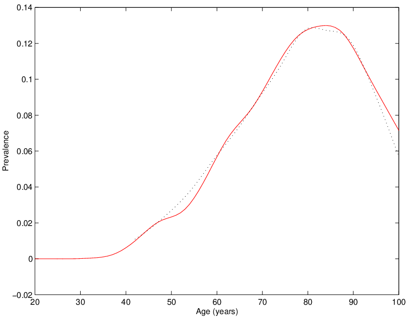
Visually this gives a fairly good agreement between the predicted curve with the actually observed age-specific prevalence. The maximum absolute deviation is 0.0146, which means that in this example the prevalence can be predicted up to 1.5 percent points. The largest deviation is in the oldest age class, when we have only a few cases of the disease.
3.2 Inverse problem
In epidemiological studies, it is more laborious to measure incidence rates than prevalences. Hence, in practice, the following inverse problem is much more important than the direct problem of the previous section. Assume in the year the functions , , and are known. Moreover, in year let the age profile of the prevalence be given. The functions and are also assumed to be known (for example from other epidemiological studies). The question then is, how well the incidence in the year can be derived from this information. For simplicity, we assume that the incidence of in can be expressed as a product
| (9) |
where The upper limit for stems from the fact, that incidence rates are non-negative. The lower limit reflects the prior knowledge, that incidence has not increased in compared to : for all Equation (9) corresponds to a proportional hazards approach, which is used widely in epidemiology.
To solve this inverse problem, we formulate an optimization problem. For given and by Eq. (9) the function is defined. If furthermore , and are known, then we are in the situation to calculate a unique function by solving the Cauchy problem described in the previous subsection 3.1. The solution of the direct problem depends on We can compare with the measured prevalence in the register. Thus, we seek for that minimizes the Euclidean distance between and
| (10) |
where .
Figure 4 shows the Euclidean distance between the prevalence in the register and the solution as a function of .

From the graph in Figure 4 it is obvious that the square of the distance is minimized at about . Since from the 50th calendar year the incidence decreases by 1% per year and a period of 20 years was considered, a factor of about is expected. The revealed value is about a factor of 1.4 too large.
4 Discussion
In this work we developed a new equation linking incidence-, remission- and mortality-rates with prevalence of a disease. In contrast to former works, the assumptions of stationary populations, independence from calendar time and zero net migration have been released. The new equation has a wide range of applicability in epidemiological, health care and health economic contexts.
However, it has several limitations. First, Eq. (5) needs the remission rate and mortality rate of the diseased to be independent from the duration of the disease. In real diseases independence from duration is only an approximation. For many infectious diseases, immune response is dependent on the time since onset of the disease. Also in chronic diseases duration since onset plays a major role. For example, the age- and sex-adjusted mortality due to coronary heart disease roughly doubles for each 10-year increase in diabetes duration. The all-cause mortality increases by a factor of 1.2 per 10-year duration, [4].
Second, although the new equation is not limited to the case , in practical applications information about the health of immigrants and emigrants is seldom obtainable. By Proposition 2.1 reasonable knowledge of prevalence in all migrants is necessary to accurately treat the case . To give an example, countries with large-scale immigration programs such as Canada observe a so-called healthy immigrant effect with respect to chronic diseases: immigrants are healthier than residents, [11]. Assumed that the emigrants from Canada have the same prevalence as the residents, it would follow However, surveys about the health status of emigrants are missing. The reason is obvious, Canada’s taxpayer-funded health care system is interested in measuring health of those who immigrate, but not in those who emigrate. Hence, information is lacking and assumptions have to be made.
Third, Eq. (5) only considers prevalence in migrants at the moment of emigration or immigration. Of course, large scale immigration is likely to change the incidence of the disease in the population, because immigrants’ health adapts to the new environment. There are many examples where immigrants from the developing countries increase incidence of diabetes and related complications when adopting westernized lifestyle, [12]. The opposite may also be true, in Canada immigrants continue to have a lower relative risk of chronic conditions compared to the native-born, even many years after immigration, [11].
Beside theoretical considerations, we use the new equation in a simulated register of a hypothetical chronic disease. The register has been simulated by Monte Carlo techniques and has been analyzed by a numerical implementation of the new equation. To check the practical applicability of the analysis, the simulation and the analysis have been strictly separated, i.e. neither was the PDE used in simulating the register, nor was information other than explicitly mentioned, used as input for the simulation exploited in the analysis. The PDE has only been used in the analysis of the direct and inverse problem. In the direct problem, the prevalence at the later point in time could be predicted from the prevalence in twenty years earlier with a high accuracy. Of course, the obtained accuracy is a result of the structure inherent to the simulation. The solution of both, direct and inverse problem, uses an affine-linear interpolation for the incidence- and mortality rates between and . In the simulated register this works well, because it reflects the trends in the incidence and mortalities. Affine-linear interpolation will impose problems if the incidence trend turns around between and . An example for a change of trends can be found in [3]: from 1995 to 2004 incidence of diabetes is found to be rising with an average of 5.3% per year in all age classes, and from 2005 to 2007 incidence is declining with 3.1% per year.
In the inverse problem, the incidence in was reconstructed from the observed prevalence in . Provided that the right-hand side of Eq. (5) is sufficiently smooth, existence of follows from the continuous dependency of the solution of the Cauchy problem on from the compact interval . Continuous dependency can be seen by noting that the solution constructed by the methods of characteristics inherits its smoothness properties from the smoothness of the right-hand side of Eq. (7), [6]. The question remains why the result (in terms of ) is about a factor 1.4 too large. The approach in solving the inverse problem is the proportional hazards assumption Eq. (9). Indeed, the simulation considers a decline of exponential type, see Eq. (8). Although the exponential in this case can approximated by an affine-linear interpolation function quite well, it appears that the solution of the inverse problem reacts quite sensitively on inaccuracies. This is in line with our observation, that the inverse problem is ill-posed [2].
References
- [1]
Brinks R (2011). A new method for deriving incidence rates from
prevalence data and its application to dementia in Germany.
http://arxiv.org/abs/1112.2720v1 - [2]
Brinks R (2012). On characteristics of an ordinary differential
equation and a related inverse problem in epidemiology.
http://arxiv.org/abs/1208.5476v1 - [3] Carstensen B, Kristensen JK, Ottosen P, Borch-Johnsen K (2008). The Danish NationalDiabetes Register: trends in incidence, prevalence and mortality. Diabetologia 51 (12):2187-96.
- [4] Fox CS, Sullivan L, D’Agostino RB Sr, Wilson PW (2004) The significant effect of diabetes duration on coronary heart disease mortality: the Framingham Heart Study. Diabetes Care 27 (3):704-8.
- [5] Gilli M, Maringer D, Schumann E (2011) Numerical Methods and Optimization in Finance. Academic Press, Waltham, MA.
- [6] Hale JK (1980) Ordinary differential equations. Robert Krieger Publishing, Malabar, FL.
- [7] Kalbfleisch JD, Prentice RL (2002) The Statistical Analysis of Failure Time Data, 2nd edn. John Wiley & Sons, Hoboken, NJ.
- [8] Keiding N, Hansen BE, Holst C (1990) Nonparametric estimation of disease incidence from a cross-sectional sample of a stationary population. Lect Notes Biomath 86: 36-45.
- [9] Keiding N (1991) Age-specific incidence and prevalence: a statistical perspective. J R Statist Soc A 154:371-412.
- [10]
Lexis W (1903) Abhandlungen zur Theorie der Bevölkerungs- und
Moralstatistik. Gustav Fischer, Jena,
http://dspace.utlib.ee/dspace/bitstream/10062/5316/4/lexis_abhandlocr.pdfAccessed 14 August 2011. - [11] McDonald JT, Kennedy S (2003) Insights into the healthy immigrant effect: health status and health service use of immigrants to Canada. Soc Sci & Med 59: 1613-27.
- [12] Misra A, Ganda OP (2007) Migration and its impact on adiposity and type 2 diabetes. Nutrition 23 (9):696-708
- [13] Murray CJL, Lopez AD (1994) Quantifying disability: data, methods and results. Bull World Health Organ 72 (3):481-494.
- [14] Murray CJL, Lopez AD (1996) Global and regional descriptive epidemiology of disability: incidence, prevalence, health expectancies and years lived with disability. In: Murray CJL, Lopez AD (ed) The Global Burden of Disease. Harvard School of Public Health, Boston, pp 201-46.
- [15] Polyanin AD, Zaitsev VF, Moussiaux A (2002) Handbook of First Order Partial Differential Equations. Taylor & Francis, London.
- [16] Preston SH, Coale AJ (1982) Age structure, growth, attrition, and accession: A new synthesis. Pop Index 48 (2):217-59.