Weighted bootstrap in GARCH models

We investigate bootstrap estimation of the parameters of GARCH processes, which are known to be able to capture the main stylized facts of observed financial series. In these models, the conditional variance is expressed as a linear function of the squared past values of the series.

It defines a stationary process for a well characterized parameter space, its most important features are presented in Section 2.

The most important question in modeling is the parameter estimation. In case of GARCH models, the QMLE estimation is the most popular one. This assumes Gaussian distribution for the observations, providing reasonable approximations even in the case of other distributions for the innovation $\eta_{t}$. We conclude Section 2 with presenting the properties of this estimator.
Of course, there are other estimation methods considered in the literature. The oldest and numerically simplest estimation method for GARCH models is the ordinary least squares (OLS). It performs poorer than the QML method and even for ARCH models the method requires moments of order 8 for the original process (Francq and Zakoian (2010), Chapter 6). An other well known method is the least absolute deviations (LAD) estimation, which outperforms the QML estimator if the innovations are Student’s $t$ distributed with 3 or 4 degrees of freedom (Peng and Yao (2003)). Ling (2007) proposed a self-weighted QML estimator for the parameters which is close in some aspects to our considerations. There are also several extensions of these estimators, see Berkes and Horvath (2004) and Francq and Zakoian (2010), Chapter 9.
Section 3 deals with the main objective of this paper, namely the investigation of bootstrap methods. Although there are different approaches for bootstrapping the GARCH models, (these will be explained in more detail in Section 3) we suggest the multiplier bootstrap approach recently proposed by Kojadinovic and Holmes (2011) for goodness of fit tests for copulas. This is a simple generalization of the standard bootstrap procedure, where the bootstrap sample is denoted by $(\tau_{ni}X_{i})$. This method is usually called weighted bootstrap and was investigated as early as in the 1990s (Barbe and Bertail, 1995; Præstgaard and Wellner, 1993).

The bootstrap weights $\tau_{ni}$ $(1\leq i\leq n,\ n\geq 1)$ are supposed to be independent from the process. We show the asymptotic normality of the bootstrap estimators under conditions, which are fulfilled in the majority of practical examples. The weighted bootstrap OLS and LAD estimators for AR(1) and ARCH processes were investigated by Bhattacharya and Bose (2012).

Other bootstrap methods for GARCH models proposed in the literature are the residual bootstrap (for instance, see Hall and Yao (2003)) and the block bootstrap (Corradi and Iglesias (2008)). These are tools for constructing confidence intervals for the parameters or for functionals of the parameters (Chen et al. (2011), Luger (2011), Pascual et al. (2006)) and for evolving goodness-of-fit tests (Luger (2011), Horvath et al. (2004)). Bootstrap methods are especially needed if the errors are heavy-tailed and this is the case in most financial applications.

Section 4 presents the results of a simulation study, where for simplicity we focus on ARCH(1) models. Here we also investigate the small-sample properties of the QMLE estimators, together with their bootstrap counterparts. This approach is practical as both the similarities and differences can be demonstrated. We give the conclusions in Section 5. The proofs can be found in the Appendix.

In this Section we summarize the needed fundamentals from the theory of GARCH processes (see Francq and Zakoian (2010) for example).

We denote the parameter vector by

which belongs to the parameter space $\Theta=(0,\infty)\times[0,\infty)^{p+q}$.
The true value of the parameters, $\theta_{0}=(\omega_{0},\alpha_{01},...,\alpha_{0q},\beta_{01},...,\beta_{0p})^{T}$ is unknown.

The GARCH($p$,$q$) process can be written in vector representation

where

$A_{t}=\left(\begin{matrix}\alpha_{1}\eta_{t}^{2}&&\cdots&&\alpha_{q}\eta_{t}^{2}&\beta_{1}\eta_{t}^{2}&&\cdots&&\beta_{p}\eta_{t}^{2}\\ 1&0&\cdots&&0&0&&\cdots&&0\\ 0&1&\cdots&&0&0&&\cdots&&0\\ \vdots&\ddots&\ddots&&\vdots&\vdots&\ddots&\ddots&&\vdots\\ 0&&\cdots&1&0&0&&\cdots&&0\\ \alpha_{1}&&\cdots&&\alpha_{q}&\beta_{1}&&\cdots&&\beta_{p}\\ 0&&\cdots&&0&1&0&\cdots&&0\\ 0&&\cdots&&0&0&1&\cdots&&0\\ \vdots&\ddots&\ddots&&\vdots&\vdots&\ddots&\ddots&&\vdots\\ 0&&\cdots&&0&0&0&\cdots&1&0\\ \end{matrix}\right)\in\mathbb{R}^{(q+p)\times(q+p)}$,

$\underline{b}_{t}=\left(\begin{array}[]{c}\omega\eta_{t}^{2}\\ 0\\ \vdots\\ 0\\ \omega\\ 0\\ \vdots\\ 0\end{array}\right)\in\mathbb{R}^{q+p}$,  $\underline{z}_{t}=\left(\begin{array}[]{c}X_{t}^{2}\\ X_{t-1}^{2}\\ \vdots\\ X_{t-q+1}^{2}\\ \sigma_{t}^{2}\\ \sigma_{t-1}^{2}\\ \vdots\\ \sigma_{t-p+1}^{2}\end{array}\right)\in\mathbb{R}^{q+p}$.

The following theorem shows that the Ljapunov exponent – thus the strict stationarity – is in connection with the existence of moments of the GARCH process, which will be helpful to verify the main results.

From now on we will concentrate on the maximum likelihood estimation of the parameters. Assume that $\{x_{1},\dots,x_{n}\}$ are observations from a GARCH(p,q) process (strictly stationary solution of the model). The Gaussian quasi-likelihood function, conditional on the $x_{1-q},...,x_{0},\tilde{\sigma}_{1-p}^{2},...,\tilde{\sigma}_{0}^{2}$ initial values, is

where the $(\tilde{\sigma}_{t}^{2})_{t\geq 1}$ are recursively defined by the following equation:

The QMLE of $\theta$ is defined as the solution $\hat{\theta}_{n}$ of

To maximize the Gaussian likelihood function, we have to minimize the following function:

Let $\mathcal{A}_{\theta}(z)$ and $\mathcal{B}_{\theta}(z)$ be the generating functions

The following assumptions A1-A6 are sufficient for the quasi-maximum likelihood estimator to have a Normal limit distribution (see Francq and Zakoian (2004)):

• A1:

  $\theta_{0}\in\Theta\text{ and }\Theta\text{ is compact}$

• A2:

  $\gamma(A_{0})<0\text{ and for all }\theta\in\Theta,\sum\limits_{j=1}^{p}\beta_{j}<1$

• A3:

  $\eta_{t}^{2}\text{ has a nondegenerate distribution and }E\eta_{t}^{2}=1$

• A4:

  $\text{If }p>0,\mathcal{A}_{\theta_{0}}(z)\text{ and }\mathcal{B}_{\theta_{0}}(z)\text{ have no common roots, }\\ \mathcal{A}_{\theta_{0}}(1)\neq 0,\alpha_{0q}+\beta_{0p}\neq 0$

• A5:

  $\theta_{0}\in\text{int}(\Theta)$

• A6:

  $\kappa_{\eta}=E\eta_{t}^{4}<\infty$.

With different assumptions, Theorem 4 was first proved by Berkes et al. (2003). Theorem 5 was proved by Berkes et al. (2003) and by Hall and Yao (2003). Hall and Yao (2003) also generalized the result to the case in which $E\eta^{4}=\infty$ and the distribution of $\eta^{2}$ is in the domain of attraction of a Gaussian or stable law with exponent $\zeta\in[1,2)$.

Although the GARCH(1,1) models perform usually better and surprisingly well against other, more sophisticated models (Hansen and Lunde, 2005, see), for the sake of simplicity we decided to illustrate the main results for stationary ARCH(1) models (special case $p$=0, $q$=1 of Definition 1). So suppose that $(X_{t})_{t\in\mathbb{Z}}$ is generated by the ARCH(1) process

where $\eta_{t}$ $(t\in\mathbb{Z})$ are i.i.d. (0,1) random variables, and $\theta_{0}=(\omega_{0},\alpha_{0})$, $\omega_{0}>0$, $\alpha_{0}\geq 0$ are the true parameters. The covariance matrix $(\kappa_{\eta}-1)J^{-1}$ of the limit distribution of the QMLE depends on the true parameters. We analyzed this dependence in stationary ARCH(1) processes, where the parameters are $\omega_{0}>0$ and $0<\alpha_{0}<1$. The matrix $J$ itself can only be approximated via simulations derived from (7): for large $N$ and simulated data $(x_{t})_{t=1,...,N}$,

Figure 1 displays the contours of the elements of the limiting covariance matrix if the innovations are Gaussian, based on $N=10^{8}$ simulations, which provides accurate results up to at least four digits. The variance of $\hat{\omega}$ and the covariance between $\hat{\omega}$ and $\hat{\alpha}$ are both more sensitive to changes in $\omega_{0}$ than in $\alpha_{0}$. The variance of the estimated parameter $\hat{\alpha}$ does not seem to depend on the true parameter value $\omega_{0}$. This is not trivial from the theoretical results, as from (7) we get

which needs further investigation.

From now on we will concentrate on the ARCH(1) process with parameters $\omega_{0}=1$ and $\alpha_{0}=0.5$. Then the limiting covariance matrix of the QML estimation is

Unfortunately (minimum) $10^{6}$ replications are needed to confidently estimate the matrix, which takes several hours for an i7 computer with 8 GB RAM memory. We will see that even the bootstrap can’t help much if we draw too few samples.
We drew $10^{6}$ samples with Gaussian innovations of size 100 to 5000 and calculated the covariance matrix of the QML estimations. Figure 2 shows that the rate of convergence drastically improves until the sample size is under 1000 and just slightly after that. We found also for other pairs of parameters that with simulations of sample size 2000, the covariance matrix can be estimated quite well, within a 1% margin.

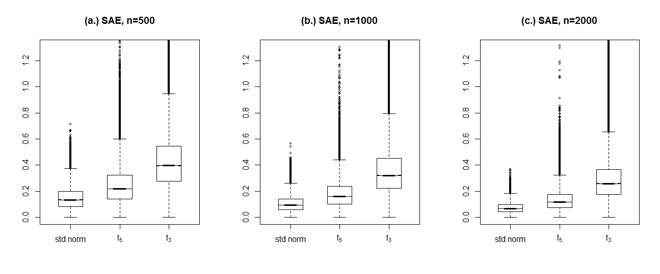
After that, 50000 samples of size n=500, 1000 and 2000 were generated with standard Gaussian and Student’s $t$ distributed innovations with 5 and 3 degrees of freedom, and we estimated the parameters with the QML method, described in Section 2. Boxplots of the sum of absolute errors (SAE) are depicted in Figure 3. The SAE is defined as $|\hat{\omega}-\omega_{0}|+|\hat{\alpha}-\alpha_{0}|$. We can see that the heavier tailes the innovations have, the larger the SAE is. Note that the Student’s $t$ errors with 3 degrees of freedom have infinite fourth moment – so Theorem 5 does not work –, but the quasi maximum likelihood estimates are fairly close on average to the original parameters. As the sample size increases, the SAEs of course become smaller. Figure 3 doesn’t display all SAE values for the Student’s $t$ innovations, the results for some samples are so bad that the SAE of the estimated parameters is more than 100.

If we take multinomially distributed weights, then the scaling factor of the covariance matrix is $\gamma=\underset{n\to\infty}{\lim}E\tau_{ni}^{2}=\underset{n\to\infty}{\lim}\left(2-\frac{1}{n}\right)=2$, therefore the quotient of the two matrices by its elements must be near 2. Figure 4 displays the convergence of the elements of the sample covariance matrix, divided element-wise by the theoretical covariance matrix (10), if the sample matrices are calculated with the multinomially weighted bootstrap (panels (a.) and (b.)) or with the residual bootstrap (panels (c.) and (d.)), for sample sizes ranging from 100 to 2000. Panel (a.) and (c.) show the convergence based on $R=1000$ samples which were bootstrapped $B=1000$ times, while the other two panels display simulations with $R=10000$ and $B=100$. The dashed lines are the sample covariance matrix values without bootstrap weights, divided by the theoretical values and scaled to 2.
Unfortunately in Theorem 5 there is not a swift convergence. In panel (a.) of Figure 4 we can’t see a straight convergence, the bootstrap can’t substantially improve the properties of the original samples, it only decreases the differences. Panel (b.) of Figure 4 helps to understand the reason: the number of samples $R=1000$ was too few. If we raise the number of samples to $R=10000$, and (for practical reasons) decrease the bootstrap repetitions to $B=100$, the convergence becomes quite good. Looking at the simulations it is not obvious which of the two bootstrap methods is the better one.

After that, we constructed 95% confidence intervals for the GARCH parameters with Gaussian innovations. Table 1 contains the average coverage percentage of confidence intervals for the parameters $\omega$ and $\alpha$ for different sample sizes (500, 1000, 2000) and using residual or weighted bootstrap methods, always compared to the Monte Carlo empirical confidence intervals. For sample size of $n=500$, the residual bootstrap outperformed the weighted bootstrap; but for sample size 2000, the residual bootstrap performed mostly better then the residual bootstrap. Using the weighted bootstrap, the average coverage of the confidence intervals improved by increasing the sample size which can’t be stated in case of residual bootstrap.

Using the limiting distributions (6) and (9) of the quasi-maximum likelihood estimator and its weighted bootstrap version, also confidence sets can be constructed. For the limiting distribution of the residual bootstrap QMLE, see Hall and Yao (2003). Table 2 reports the average coverage of the confidence sets, the row ’Empirical’ contains the 95% and 99% coverage of R=1000 samples, while the other two rows show the coverage of residual and weighted bootstrap QML estimates with $R=1000$ samples and $B=1000$ bootstrap replications. Note that in each case the weighted bootstrap QMLEs performed a bit better than the residual ones. Figure 5 represents the estimated pairs of parameters ($\hat{\omega},\hat{\alpha}$) and the 95% and 99% confidence sets – according to the limiting distribution – for different sample sizes (500, 1000, 2000). It can be seen that the confidence ellipses have a leaning longitudinal axis and the larger the sample size is, the smaller the ellipses become. The figures a.)–c.) were plotted for $R=1000$ samples and the figures d.)–f.) were plotted for the weighted bootstrap QMLEs, bootstrapped $B=100$ times. Compared the points against the coverage sets, the coverage looks quite decent, and there are no clusters on the outside of the ellipses.

We have demonstrated that the multiplier bootstrap method reflects well the properties of the original QMLE estimator, thus it may be used for investigating the estimators in practical problems (we plan to come back to this issue in another paper soon).

Another important observation of our simulations is that the asymptotic results presented in Sections 2 and 3 can be used for sample sizes in the range of thousands only, as for smaller samples the deviations may still be substantial.

It is also worth mentioning that we have found an interesting dependence between the asymptotic covariance matrix and the parameter values themselves, which should be taken into account in practical applications.

The work was supported by the European Union Social Fund (Grant Agreement No.TÁMOP 4.2.1/B-09/1/KMR-2010-0003).

Proof of Theorem 6.
We follow the proof of Francq and Zakoian (2004) and go into details only when changes are necessary. See the original proof in their paper or in their book (Francq and Zakoian (2010)) on pages 156-159.

First, we introduce some notations to write the system of equations

in matrix form.

$\underline{\sigma}_{t}^{2}:=\left(\begin{array}[]{c}\sigma_{t}^{2}\\ \sigma_{t-1}^{2}\\ \vdots\\ \sigma_{t-p+1}^{2}\end{array}\right),\ \underline{c}_{t}^{2}:=\left(\begin{array}[]{c}\omega+\sum\limits_{i=1}^{q}\alpha_{i}X^{2}_{t-i}\\ 0\\ \vdots\\ 0\end{array}\right),\ B:=\left(\begin{array}[]{cccc}\beta_{1}&\beta_{2}&\cdots&\beta_{p}\\ 1&0&\cdots&0\\ \vdots&\ddots&\ddots&\vdots\\ 0&\cdots&1&0\end{array}\right).$

So we have

Let us denote by $B_{k}(\theta)$ the open sphere with center $\theta$ and radius $k$.

The proof consists of five steps and we also need a modification of the ergodic theorem.

(I.) The initial values are asymptotically irrelevant

Iterating (11), we get that for some appropriate $K>0$ and $0<\rho<1$

To prove (12), it is sufficient to show that

and

For arbitrary $\delta>0$

and

In the estimation above we applied Markov’s inequality and Theorem 3.
Using the Borel-Cantelli lemma, we get

and

Finally, using Cesaro’s lemma, (14) and (15) are proved.

(II.) Identifiability of the parameter

For details, see Francq and Zakoian (2010), page 158.

(III.) The log likelihood function is integrable at $\theta_{0}$ and it has a unique minimum at the true value

It is easy to show that $E_{\theta_{0}}I_{n}^{*}(\theta)=E_{\theta_{0}}l_{nt}^{*}(\theta)\in\mathbb{R}\cup\{\infty\}$, because

The log likelihood function is integrable at $\theta_{0}$:

The limit criterion is minimized at the true value $\theta_{0}$

where the equality holds iff $\sigma_{t}^{2}(\theta)\overset{P_{\theta_{0}}-a.s.}{=}\sigma_{t}^{2}(\theta_{0})$ and as a consequence of (II.), this is equivalent to $\theta\overset{P_{\theta_{0}}-a.s.}{=}\theta_{0}$.

(IV.) For any $\theta\neq\theta_{0}$, there exists a neighborhood $V(\theta)$ such that

To prove this, we use (I.) and a consequence of the ergodic theorem.

In the last equation, we used that $\underset{\theta}{\text{inf }}l^{*}_{nt}(\breve{\theta})$ is an ergodic process. The expression $\underset{\breve{\theta}\in V_{1/k}(\theta)\cap\Theta}{\text{inf}}l_{1}(\breve{\theta})$ is monotonically increasing in $k$, so $E_{\theta_{0}}\underset{\breve{\theta}\in V_{1/k}(\theta)\cap\Theta}{\text{inf}}l_{1}(\breve{\theta})$ is also monotonically increasing and using Beppo Levi’s theorem,

(V.) Last step of the proof, using the compactness of $\Theta$.
For any neighborhood $V(\theta_{0})$ of $\theta_{0}$,

As $\Theta$ is a compact set, by definition, there exist $V(\theta_{0}),V(\theta_{1}),...,V(\theta_{k})$ open subsets of $\mathbb{R}^{p+q+1}$, for which $\Theta\subseteq\left(\cup_{i=0}^{k}V(\theta_{i})\right)$ and $V(\theta_{1}),...,V(\theta_{k})$ satisfy (IV.). So

As a consequence of (IV.) and (16), for $n$ large enough $\breve{\theta}_{n}^{*}$ $\in$ $V(\theta_{0})$ with probability 1. This is true for any neighborhood $V(\theta_{0})$, therefore

Proof of Theorem 7.
We follow the proof of Francq and Zakoian (2004) and go into details only when changes are necessary. See the original proof in their paper or in their book (Francq and Zakoian (2010)) on pages 159-168.
The Taylor-expansion of the function $\tilde{l}_{nt}^{*}(\theta)$ around $\theta_{0}$ is

where $\breve{\theta}$ is between $\theta_{0}$ and $\theta$.
Derivating, summarizing and multiplying this equation with $\frac{1}{\sqrt{n}}$, we get

where $\breve{\theta}$ is between $\theta_{0}$ and $\hat{\theta}^{*}_{n}$.
We will show that

References

• Barbe and Bertail (1995) P. Barbe and P. Bertail. The weighted bootstrap, volume 98. Springer, 1995.
• Berkes and Horvath (2004) I. Berkes and L. Horvath. The efficiency of the estimators of the parameters in GARCH processes. The Annals of Statistics, 32(2):633–655, 2004.
• Berkes et al. (2003) I. Berkes, P. Kokoszka, et al. GARCH processes: structure and estimation. Bernoulli, 9(2):201–227, 2003.
• Bhattacharya and Bose (2012) A. Bhattacharya and A. Bose. Resampling in time series models. Arxiv preprint arXiv:1201.1166, 2012.
• Chen et al. (2011) B. Chen, Y.R. Gel, N. Balakrishna, and B. Abraham. Computationally efficient bootstrap prediction intervals for returns and volatilities in ARCH and GARCH processes. Journal of Forecasting, 30(1):51–71, 2011.
• Corradi and Iglesias (2008) V. Corradi and E.M. Iglesias. Bootstrap refinements for QML estimators of the GARCH (1, 1) parameters. Journal of Econometrics, 144(2):500–510, 2008.
• Francq and Zakoian (2004) C. Francq and J.M. Zakoian. Maximum likelihood estimation of pure GARCH and ARMA-GARCH processes. Bernoulli, 10(4):605–637, 2004.
• Francq and Zakoian (2010) C. Francq and J.M. Zakoian. GARCH models: structure, statistical inference and financial applications. Wiley, 2010.
• Hall and Yao (2003) P. Hall and Q. Yao. Inference in ARCH and GARCH models with heavy–tailed errors. Econometrica, 71(1):285–317, 2003.
• Hansen and Lunde (2005) P.R. Hansen and A. Lunde. A forecast comparison of volatility models: does anything beat a GARCH (1, 1)? Journal of applied econometrics, 20(7):873–889, 2005.
• Horvath et al. (2004) L. Horvath, P. Kokoszka, and G. Teyssiere. Bootstrap misspecification tests for ARCH based on the empirical process of squared residuals. Journal of Statistical Computation and Simulation, 74(7):469–485, 2004.
• Kojadinovic and Holmes (2011) Yan J. Kojadinovic, I. and M. Holmes. Fast large-sample goodness-of-fit tests for copulas. Statistica Sinica, 21:841–871, 2011.
• Ling (2007) S. Ling. Self-weighted and local quasi-maximum likelihood estimators for ARMA-GARCH/IGARCH models. Journal of Econometrics, 140(2):849–873, 2007.
• Luger (2011) R. Luger. Finite-sample bootstrap inference in GARCH models with heavy-tailed innovations. Computational Statistics & Data Analysis, 2011.
• Pascual et al. (2006) L. Pascual, J. Romo, and E. Ruiz. Bootstrap prediction for returns and volatilities in GARCH models. Computational Statistics & Data Analysis, 50(9):2293–2312, 2006.
• Peng and Yao (2003) L. Peng and Q. Yao. Least absolute deviations estimation for ARCH and GARCH models. Biometrika, 90(4):967–975, 2003.
• Præstgaard and Wellner (1993) J. Præstgaard and J.A. Wellner. Exchangeably weighted bootstraps of the general empirical process. The Annals of Probability, 21(4):2053–2086, 1993.