Non Gaussianity and Minkowski Functionals: forecasts for Planck
Abstract
We study Minkowski Functionals as probes of primordial non-Gaussianity in the Cosmic Microwave Background, specifically for the estimate of the primordial ‘local’ bi-spectrum parameter , with instrumental parameters which should be appropriate for the Planck experiment. We use a maximum likelihood approach, which we couple with various filtering methods and test thoroughly for convergence. We included the effect of inhomogeneous noise as well as astrophysical biases induced by point sources and by the contamination from the Galaxy. We find that, when Wiener filtered maps are used (rather than simply smoothed with Gaussian), the expected error on the measurement of should be as small as when combining the 3 channels at 100, 143 and 217 GHz in the Planck extended mission setup. This result is fairly insensitive to the non homogeneous nature of the noise, at least for realistic hit-maps expected from Planck. We then estimate the bias induced on the measurement of by point sources in those 3 channels. With the appropriate masking of the bright sources, this bias can be reduced to a negligible level in the 100 and 143 GHz channels. It remains significant in the 217 GHz channel, but can be corrected for. The galactic foreground biases are quite important and present a complex dependence on sky coverage: making them negligible will depend strongly on the quality of the component separation methods.
Keywords:
Cosmology: Cosmic Microwave Background, Minkowski functionals; Methods: statistical, numerical1 Introduction
The Planck satellite was launched in May 2009 (Tauber et al., 2010; Planck Collaboration et al., 2011a) to observe the microwave sky and particularly the Cosmic Microwave Background (hereafter CMB). It will provide major pieces of information about the early evolution of the universe and the origin of structures thanks to its unprecedented combination of resolution, sensitivity, and spectral coverage. One of the important objectives of this mission is to bring new constraints on inflation theory and primordial non Gaussianities. In the simplest inflationary models based on a single slowly rolling scalar field, primordial fluctuations should be only weakly non Gaussian (Maldacena, 2003; Bartolo et al., 2006). Yet in more general models a much higher level of non-Gaussianity (hereafter NG) is expected. We can cite models with multiple scalar fields, features in the inflaton potential, non-adiabatic fluctuations, non-standard kinetic terms, warm inflation, deviations from Bunch-Davies vacuum (review in Bartolo et al. 2004) or completely different mechanisms, for example topological defects such as cosmic strings (Kaiser & Stebbins, 1984).
Non-Gaussianity is often parametrised in a phenomenological way by the non-linear ‘local’ coupling parameters , , … which appear in the perturbative development of the primordial curvature perturbation (Komatsu & Spergel, 2001; Okamoto & Hu, 2002),
| (1) |
where is the linear Gaussian part of the Bardeen curvature. We will focus here on constraining the first parameter, .
The latest results from WMAP (Komatsu et al., 2011) with 7 years of data provide the constraint
| (2) |
at the 68% confidence level. With Planck, we expect the error on to be at best of the order of from both temperature and polarisation (Yadav & Wandelt, 2010; Sefusatti et al., 2009) or of the order of for the temperature only (Komatsu & Spergel, 2001). These constraints on were obtained with bi-spectrum measurements (Komatsu et al., 2005; Yadav et al., 2007; Yadav et al., 2008). The CMB bi-spectrum is the harmonic transform of the three-point correlation function and it has been shown that this is theoretically an optimal estimator for as it saturates the Cramér-Rao inequality for a weak non Gaussianity (Babich, 2005).
However, alternative statistics to the bi-spectrum have been also developed, that can at least serve as checks and diagnoses of the results obtained from the bi-spectrum. One of the main reasons to study various probes of non Gaussianity is indeed that they are affected differently by different systematics and contaminants such as inhomogeneous noise and foreground residuals induced by our galaxy and point sources, as well as secondary anisotropies (e.g., Aghanim et al., 2008, and references therein) such as integrated Sachs-Wolfe effect, Sunyaev-Zeldovich effect (Sunyaev & Zeldovich, 1972) and weak gravitational lensing, which can all contribute to non Gaussianity of the CMB in a non trivial way. In particular, the most serious bias on from secondary anisotropies arises from the coupling between weak gravitational lensing and integrated Sachs-Wolfe effect (Goldberg & Spergel, 1999; Serra & Cooray, 2008; Hanson et al., 2009; Mangilli & Verde, 2009; Munshi & Heavens, 2010, see), which adds complexity to the analyses.
Here we focus on a complete set of topological tools, the Minkowski Functionals (hereafter MFs) introduced in cosmology by Mecke et al. (1994). MFs describe the morphological features of random fields over excursion sets, i.e. regions where the field exceeds some threshold level . These well-known probes of primordial non-Gaussianities (Schmalzing & Buchert, 1997; Winitzki & Kosowsky, 1998; Schmalzing & Gorski, 1998) have been widely used in two and three dimensions, for instance on WMAP CMB data (Hikage et al., 2006; Hikage et al., 2008) and on the SDSS galaxy catalogue (Park et al., 2005; Hikage et al., 2006).
For CMB studies, MFs provide a nice complement to the bi-spectrum for several reasons. Firstly, at variance with the bi-spectrum, which evolves in harmonic (or Fourier) space, MFs are defined in real space, which makes a robust implementation for MFs in practice much easier than for the bi-spectrum. Secondly, MFs are sensitive to the full hierarchy of higher-order correlations, instead of third order only, and can provide additional information on all the non-linear coupling parameters beyond the sole . Because they are measured on excursions of the density field smoothed with an isotropic window, MFs only probe angular averages of higher order statistics, leaving out the angular dependences, at variance with the bi-spectrum. This explains why MFs are less optimal than the bi-spectrum in terms of disentangling between various models of weak NG. However, the very nature of these angular averages eases considerably statistical analysis and reduces the number of parameters while performing maximum likelihood analysis. As a result, even though suboptimal, MFs represent powerful tools of investigation of NG. For instance, the first limit on the primordial non-Gaussianity in the isocurvature perturbation was measured with MFs, even though theoretical predictions where computed on the bi-spectrum (Hikage et al., 2009). Note finally that the constraint on obtained from the analysis of WMAP3 with MFs reads
| (3) |
at the 68% confidence level (Hikage et al., 2008), a rather competitive result, after all, compared to the bi-spectrum constraints from WMAP7 (eq. 2).
In this paper, we investigate constraints on obtained with MFs from a practical point of view, in order to ease at best future application of MFs to Planck data. After detailing the MFs estimators and the Bayesian method we implemented, we review the effects of the main systematics that can affect/bias the results. These systematics can be of instrumental nature –inhomogeneous noise, beams– or of astrophysical nature: the observed microwave sky contains foreground emission from the Milky Way and from extragalactic sources.
Our Galaxy is indeed a strong source of contamination. It is generally accounted for by masking and/or by using component separation methods and by assuming that the final residual bias on is negligible compared to error bars (Hikage et al., 2008; Komatsu et al., 2003). Nevertheless it has been shown that component separation leave Galactic features in CMB maps (Chiang et al., 2003). Indeed the various methods of component separation (Leach et al., 2008) need to be controlled at the new level of accuracy on expected for Planck. Another approach is to use foreground templates and to marginalise over them (Komatsu et al., 2002; Komatsu et al., 2011). Here, we chose to analyse the behaviour of MFs when using masks and a naïve model of component separation. For that, we used foreground templates provided by the Planck Sky model (PSM) code (Delabrouille et al, 2012).
Point sources are mostly unresolved galaxies (at least in low-density regions of Galactic emission), some emitting a signal sufficiently high to be detected individually, the others forming a diffuse unresolved background. Point sources consist first of radio-galaxies, active galactic nuclei which emit in radio frequencies with synchrotron process. They can also be dusty starburst galaxies which are observed via the thermal emission of their dust heated by the ultra-violet emission of young stars. Current instruments are not able to detect all these galaxies individually and the integrated emission of all the faint galaxies form a diffuse background, the Cosmic Infrared Background (CIB) which has been recently studied and observed (Puget et al., 1996; Lagache & Puget, 2000; Planck Collaboration et al., 2011c). The strong point sources are accounted for by masking them but the fainter ones can still induce biases in NG studies. The point source bi-spectrum has already been measured (Komatsu et al., 2011) and its effect in the estimates of evaluated, for bi-spectrum measurements (Babich & Pierpaoli, 2008; Serra & Cooray, 2008; Lacasa et al., 2012).
In addition to these contributions, as mentioned above, CMB contains secondary anisotropies imprinted between the surface of last scattering and present time. While we leave the treatment of these secondary anisotropies for future work, we shall treat in detail the contamination from our galaxy and point sources.
This paper is organised as follows. In section 2, we review the Bayesian method we use to optimise the constraint on from MFs. In section 3, we study the effects of pixelisation and filtering. Section 4 deals with the effect of inhomogeneous noise. In sections 5 and 6, we study astrophysical sources of systematic effects: first point sources, then Galactic foregrounds. Section 7 summarises and discusses the results. For completeness, some additional technical details can be found in Appendix A, which discusses analytic predictions for MFs in the weakly non Gaussian regime, Appendix B, which details the algorithm used to measure MFs, Appendix C, with a convergence study of our , and Appendix D, which provides some details on the Planck simulation experiments performed in this work.
The pixelisation scheme adopted in this paper is the same as in Planck processed maps, namely HEALPix11 1 Available at http://healpix.jpl.nasa.gov (Górski et al., 2005).
Note finally that there are a number of tables to illustrate the results. Some of these tables are purposely incomplete to lighten the presentation.
2 Method
In this section, we set notations by first recalling basics of Minkowski functionals and their measurement inside an excursion of varying height (§ 2.1). Then we detail the Bayesian approach we use to estimate (§ 2.2), by comparing the measurement of a functional or a combination of functionals to its expected value. Within a set of reasonable simplifying assumptions, in particular weak non Gaussianity, this approach reduces to a simple test (§ 2.2.1). The numerical estimate of this requires the accurate calculation of the covariance matrix of our estimator from a large set of Gaussian simulations, as discussed in § 2.2.2. Additional details concerning the Gaussian simulations set up as well as the method used to test the convergence of the are given in Appendix C. Once we have a numerically robust test, we study its sensitivity to important parameters of the problem, such as the number of bins used to explore the excursion and the range of the excursion levels, as well as the choice of the functionals and/or their combination (§ 2.3).
2.1 Minkowski Functionals
For a two-dimensional field of zero mean and of variance , defined on the sphere, and smoothed with a window of typical size (to be defined later), we consider an excursion set of height , i.e. the set of points where the field exceeds the threshold . In what follows, we shall study the topological properties of the excursion with four quantities, denoted by (). The first three ones correspond to MFs: is the fractional Area of the regions above the threshold, is the Perimeter of these regions and is the Genus, defined as the total number of connected components of the excursion above the threshold minus the total number of connected components under the threshold. The fourth one, that will be called the Number of clusters, also noted , is just the number of connected regions above the threshold for positive thresholds and reversely for negative thresholds (Chingangbam et al., 2012, these regions are also known as Betti numbers or as cold/hot spots,). Analytic formulae (theoretical expectation values) for the quantities are known for Gaussian and weakly non Gaussian fields and are summarised in Appendix A. An interesting property of these functionals is that the pure spectral dependence can be factorised out:
| (4) |
where the amplitude is determined by the shape of the power-spectrum of the field fluctuations. The renormalised functionals depend only on the non Gaussian corrections, i.e. on the behaviour of correlations functions beyond second order. The analysis of allows us to focus on non Gaussianity, which is the goal of this paper.
2.2 Testing non Gaussianity with a
To provide constraints on non-Gaussianity, we adopt a Bayesian approach similar to that of Hikage et al. (2008), comparing measurement of normalised functionals on the data map under consideration to the “theoretical predictions” obtained from the average of measurements of on a large number of non-Gaussian simulations, the non Gaussian part being simply proportional to . We will focus here on the non-linear coupling parameter ‘local’ but the method can be applied to other types of non Gaussianities.
To perform the measurements, we consider an ensemble of values of ranging from and , defining a vector for each of the functionals. The statistics under consideration will then be a vector of elements, if only one functional is used in the analysis, or if a combination of functionals is considered.
The Bayes formula writes
| (5) |
In what follows, we shall take a flat prior for , with a constant, while the evidence will be just considered as a normalisation.
2.2.1 Construction of a test
We assume that the likelihood is a Gaussian, which allows us to define a simple test for . This approximation is expected to be good in the regime where the fluctuations of each component of the vector remain small compared to its ensemble average , when one considers a large number of realisations of the random field. Keeping these fluctuations small sets practical constraints on (i) the value of , which should not be too extreme to avoid sensitivity to rare events, (ii) the smoothing scale , that should be small enough to probe a sufficient number of independent harmonic modes on the sky. Because we consider only small values of in most of what follows our main concern is the choice of . We shall restrict to the range (Gott et al., 1990, see also the discussion in).
With all these simplifications, the posterior becomes
| (6) |
with
| (7) | |||||
| (8) |
where is the model under test. It can be derived analytically in the weakly non Gaussian regime (see Hikage et al., 2008, and appendix A) or by direct measurements on simulations. Since we want to take into account complex additional contributions such as inhomogeneous noise and masks, we use here the more flexible second approach with non-Gaussian simulations provided by Elsner & Wandelt (2009). So is the mean of measured over maps with a level non-Gaussianity . In practice, we shall take
| (9) |
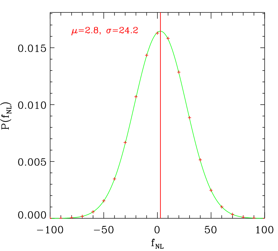
Since non-Gaussianity is weak (Komatsu et al., 2011), one can compute the covariance matrix in a Monte-Carlo fashion relying on simulations of Gaussian maps of the CMB (to which we add, when relevant, beam effects, noise, masks). In that case, the posterior probability distribution function is expected to be very close to a Gaussian, as illustrated by Fig. 1 for the Perimeter. Indeed, in the weakly non Gaussian regime, is, at first order, a linear function of (see, e.g., Appendix A).
To estimate the most likely posterior value of and an uncertainty, instead of trying to find iteratively the maximum of followed by an estimate of the local curvature using e.g. the Fisher information matrix to estimate the error, we prefer, for simplicity and robustness, to compute directly the average and the variance of the posterior distribution, . This latter is estimated using a number of equally spaced bins, , , with, for the purpose of this paper . From this approximation of the posterior, the average and the variance are directly estimated numerically via the simple formulae
| (10) | |||||
| (11) |
where is proportional to .
Finally, one might consider performing a number of realisations of the data –also called in this paper “test” maps– to have a more accurate description of the “typical” expected posterior probability. However such a forecasting is not obvious, as we have to define a frequentist average over Bayesian quantities, to predict the typical value expected for and . Our choice, equivalent to Fisher information forecast in the pure Gaussian case, consists in estimating and from the following averages
| (12) | |||||
| (13) |
where and are obtained from the analysis of “data” map number using eqs. (10) and (11). In what follows, we shall always take (for each individual value of considered in the tests maps)
| (14) |
2.2.2 Convergence issues
The covariance matrix is estimated from the average over simulations, on each of which a vector of functionals is measured:
| (15) |
with .
The calculation of the requires the inversion of the covariance matrix, an uneasy task, because can be ill-conditioned, especially if is not large enough. The number of simulations required to have a good estimate of the function indeed depends on the number of bins, , on the functionals under consideration, their number, , and on the choice of . The way we estimate is exposed in detail in Appendix C. The results of our analyses are summarised in table 1, where the minimum values of required for having a better than two percent accuracy on the obtained from the perimeter are displayed for various realistic set-ups in terms of the number of bins and of the excursion range. Similar orders of magnitude are expected for other functionals or when combining a set of functionals, as explicitly checked for the combination , and , where the corresponding value found in Table 1 remains unchanged within 5%. This latter property comes from the fact that in practice, two different functionals are much less correlated than the same functional estimated at two successive bins of the excursion: combining functionals doubles the dimensions of matrix but does not make it significantly more degenerate. In the subsequent calculations performed in this paper, we shall take
| (16) |
a number of simulations sufficient for a good estimate of the for and .
2.3 Sensitivity of the estimator
In this section we discuss the sensitivity of our estimator, that is the uncertainty on the estimated , with respect to the number of bins, , the excursion range, , and the set of functionals used, whether it is the Area, the Perimeter, the Genus, the Number of clusters, or a arbitrary combination of any of them. Our simulation setup is the same as in the previous paragraph (and detailed in Appendix C). We checked, in this full sky configuration with homogeneous noise, that our estimator is unbiased, (within numerical limits set by the finiteness of and ).
The results of our analyses are displayed in Tables 2 and 3. They show that the combination
| (17) |
is fairly optimal and shall represent our choice in the subsequent analyses. Note that it is important to notice that assuming the covariance matrix to be diagonal, as done for instance in Eriksen et al. (2004); Gott et al. (1990) is not a good approximation in the case of and decreases by more than a factor two the constraining power of the .
The comparison between various functionals lead to the following ranking, in term of discriminative power:
| (18) |
While the Perimeter, the Genus and the Number of cluster present the same order of sensitivity, the Area is about twice less discriminative than them. Most of the information on can be extracted by a combined analysis of the perimeter and the genus, , with a little improvement when taking into account the number of clusters, , but the area does not carry significant pieces of additional information compared to the three others.
| 29 | 25.5 | 25 | 25 | |
| 27 | 25 | 25 | 25 | |
| 37.5 | 37 | 37 | 36.5 |
| Functionals | ||
|---|---|---|
| 44 | ||
| 25 | ||
| 25 | ||
| 28 | ||
| 20 | ||
| 19 | ||
| 18.5 |
3 Filtering and smoothing
The measurement of Minkowksi Functionals requires smoothing of temperature maps in order to remove the contribution of the noise. This smoothing is performed at various scales on a pixelised map in order to extract all the statistical information available. First, one has to deal with discreteness effects brought by the pixelisation. In § 3.1, we show that for practical measurements, it is not needed to have a large value of HEALPix resolution parameter to extract all the relevant information even if this means a pixel size comparable to the size of the smoothing window: this is because we explicitly account for these pixelisations effects in the model. In § 3.2, we consider Gaussian smoothing and show that most information on obtained from MFs is present at the smallest possible scales, i.e. at scales comparable to the size of the beam of the instrument. Note however that this result stands for local and might vary for different types of non Gaussianity. Finally, § 3.3 deals with Wiener filtering for the field, its first and second derivatives. We show that the results obtained with a simple combination of Wiener filters set much better constraints on than naïve Gaussian smoothing at various scales.
In what follows, smoothing scale will be expressed in units of the full width at half maximum (FWHM), (see Appendix D.2 for more details).
3.1 Pixelisation effects: choice of
In principle, the pixel size should be small compared to the smoothing kernel size, in order to avoid systematic errors introduced by the discrete nature of the pixelisation (Colombi et al., 2000; Novikov et al., 2006, see, e.g.). We checked in practice that no bias is introduced on the measurement of even when the pixel size becomes comparable to the smoothing window size, because the defects of the pixelisation are present as well in the model. However, introducing larger pixels is similar to coarse graining and decreases the effective level of statistical richness, which in turn increases the uncertainty on . Furthermore, a too large pixel size would simply make the additional filtering operation inoperative: instead, what we would get in that case is simply the dominant part of filtering to be a convolution with a top-hat of the pixel shape.
Table 4 gives the error obtained on when using the combination of all four functionals, for various values of HEALPix resolution parameter , different levels of noise and a Gaussian smoothing with . For Planck purpose, we also find that the improvement brought by the resolution is tiny, as expected for higher level of noise, and this table shows that it is not needed in practice to go beyond , which is rather handy computationally speaking. From now on, unless specified otherwise, we shall assume
| (19) |
for all subsequent analyses.
| Noise | |||
|---|---|---|---|
| 0.33 K.deg | 19.5 | 16.5 | 16 |
| 0.5 K.deg | 20 | 16.5 | 16.5 |
| 0.7 K.deg | 20 | 17 | 16.5 |
| 1.1 K.deg | 20 | 18.5 | 18 |
3.2 Gaussian Smoothing
Smoothing with a Gaussian kernel depends only on angular scale, . A priori, each type non-Gaussianity is characterised by a specific scale range where the sensitivity of the estimator of is the best and we have to stay aware that we are limited here to only one particular case of non Gaussianity, although quite typical.
We tested different smoothing scales, including even very small scales (), smaller than size of the beam ( in the case of the combined channels), and just above the size of the pixel, which might look awkward, but in fact does not introduce any significant bias on the measurement of , as already argued in § 3.1 when discussing about pixelisation effects.
One issue about smoothing at large scales is that it reduces the number of independent modes available on the sky. This in turns reduces the quality of the measurement of the MFs in the tails (large values of ) and can make the likelihood function non Gaussian, as discussed in the beginning of § 2.2.1, particularly if is too large. For instance, with , the Gaussian assumption for the likelihood is legitimate for but not for . Here we checked that our analysis was still valid and well converged at smoothing scales as large as for our default choice for the parameters, , and .
Table 5 summarises the results of our analyses for the case when the combination of all functionals is used at various scales or various combinations of scales. Note that when combining 4 scales, we have a large number of entries in the data vector, , but we checked that this did not affect the convergence of the calculation of the covariance matrix with . The results of Table 5 show that there is no significant statistical information for . Most of the signal is captured by the combination with .
Note that the scales we consider here are much smaller than those considered in Table 3 of Hikage et al. (2006) that correspond to , which explains the better constraints we obtain on .
| 5’ | 16.5 | |
| 10’ | 20 | |
| 20’ | 26.5 | |
| 40’ | 34 | |
| 5’ + 10’ | 14 | |
| 5’ + 10’ + 20’ | 13.5 | |
| 5’ + 10’ + 20’ +40’ | 13.5 |
3.3 Wiener filters
Now we consider Wiener filtering, which is an optimal way of recovering the signal of a data map in case both the underlying signal and the noise are Gaussian. The Wiener filter writes, in harmonic space,
| (20) |
where is the forecasted power-spectrum of the signal we want to analyse and is the known power spectrum of the noise. Here, signal will refer to the dominant, Gaussian, cosmological part of the CMB. Obviously, this is sub-optimal, since we are after the non Gaussian part of the CMB, while all the rest should be considered as noise. However, using a Wiener filter designed for extracting the non Gaussian signal would require a stronger prior, making the measurement of potentially more accurate but only for a restricted class of non Gaussianities.
Similarly, one can define in harmonic space a “derivative” Wiener operator,
| (21) |
and a “second derivative” Wiener filter optimal for recovering the Laplacian of the signal, ,
| (22) |
In practice, we use a smoothed version of the quantity , a “Wiener-like” function used for component separation method (CMB removal) in Planck HFI Core Team et al. (2011). Before applying the Wiener filters we also correct the map for the Gaussian beam corresponding to the channel configuration. The three resulting filters, , and are represented on Fig. 2.
Table 6 summarises the results of our analyses using them. It shows, not surprisingly, that alone does much better than Gaussian smoothing (Table 5) and a significant improvement is obtained when combining with resulting in an overall reduction of the error on of 30% compared to the best results obtained with Gaussian smoothing. On the other hand, does not bring anything interesting, but this is somewhat expectable: for a stationary and isotropic random field, there is no correlation between the field and its first derivatives, but there is a strong correlation between the field and its second derivatives.

| Functional | ||||||
|---|---|---|---|---|---|---|
| 51 | ||||||
| 14 | ||||||
| 21 | ||||||
| 20 | ||||||
| 13 | ||||||
| 12.5 | 32 | 27 | 9 | 12.5 | 9 |
4 Inhomogeneous Noise
Due to the scanning strategy and the orientations of the different horns and bolometers (Dupac & Tauber, 2005), the distribution of the noise in the raw sky maps is correlated, anisotropic and inhomogeneous. In what follows, we treat effects of inhomogeneity and anisotropy of the noise, by relying on hitmaps (Keihänen et al., 2005, generated with the software MADAM of), in which each pixel value represents the number of times the pixel has been observed by the satellite. Our modelling of the noise in each pixel of the map then reads
| (23) |
Note thus that, since correlations are neglected, anisotropy of the noise is modelled only partly, through the anisotropy of the hit map. Even more realistic analyses would take into account of the effects of correlations in the noise, which will be addressed in future work. Figures 3 and 4 show a hit map and the corresponding noise map for the 143 GHz channel in a simulation of Planck signal (Planck HFI Core Team et al., 2011, which used the characteristics of the instrument described in).


To analyse the impact of various levels of realism in modelling of the noise on the determination of , we consider two configurations: one where inhomogeneous noise is included in all the steps of the analysis, and one where only each of the test maps has its own realisation of inhomogeneous noise -- relying on the same hit map22 2 The one obtained in the 143 GHz channel, to be specific. but with different random seeds. We test here the null hypothesis but we checked that the conclusions do not change significantly for other values of . All the simulations are performed as detailed in Appendix D for full sky surveys with no foregrounds, , and a Gaussian smoothing with to filter out the noise, which corresponds to a rather (almost the most) pessimistic case in terms of inhomogeneous noise.
The results of our analyses are summarised in table 7 and table 8 for four levels of noise which are likely to bracket the actual sensitivity of Planck. To understand the results displayed in the tables, Figures 5 and 6 compare the effect of neglecting inhomogeneous noise to the presence of a “true” on the functionals for the nominal mission in the 143 GHz channel.
The Area functional, , seems fairly insensitive to the effect of the inhomogeneity of the noise, which in turns makes the determination of from the Area quite robust to that respect. This is not very surprising: the area is proportional to the cumulated one point distribution function (pdf). The presence of inhomogeneous noise locally induces a convolution of this pdf with a Gaussian of varying width depending on the value of the number of hits in the map. The effect of this convolution is negligible when the r.m.s. of the local noise is small compared to the r.m.s. of the field under consideration.33 3 Note that this argument would be valid as well for a non Gaussian noise. Here this is the case: the additional Gaussian smoothing with reduces the typical local rms of the smoothed noise map to whatever the channel considered, to be compared to .
The examination of Fig. 5 shows that other functionals are rather sensitive to the effect of inhomogeneous noise, which is also expected. Indeed, we can guess that the presence of inhomogeneous noise augments the contrasts between cold and hot spots compared to the homogeneous case, hence building up a signal in , and . However, this signal is also contained in the parameter in eq. (4) which tends to compensate for the effect on . Hence, the normalised functionals, , appear to be less affected by inhomogeneous noise than the “raw” functionals, , as illustrated by Fig. 6. There is still some rather significant residual signal, at least for the small smoothing scale considered here. However, the parity of the black curves in the different panels of Fig. 6 is opposite to that of the curves corresponding to a true primordial (green and red curves): we do not expect in that case the presence of inhomogeneous noise to introduce any bias on the measurement of . These simple statements are confirmed by the examination of Table 7. On the other hand, the presence of inhomogeneous noise makes the uncertainty on slightly larger, increasingly with the average level of noise, as shown in Table 8. Fortunately, for the three combined channels in extended Planck mission, the effects of the inhomogeneity of the noise become nearly negligible and can be fairly ignored, as we shall do from now on.
| Noise (K.deg) | 1.1 | 0.7 | 0.5 | 0.33 | ||||
|---|---|---|---|---|---|---|---|---|
| Functional | ||||||||
| 1 | 38.6 | |||||||
| -4 | 23.6 | |||||||
| -0.4 | 22 | |||||||
| -0.2 | 24.7 | |||||||
| -4.4 | 18.8 | -3.8 | 17.9 | -2.3 | 17 | -0.8 | 16.7 | |
| Noise (K.deg) | 1.1 | 0.7 | 0.5 | 0.33 | ||||
|---|---|---|---|---|---|---|---|---|
| Functionals: | ||||||||
| Configuration 144 4 For the reference maps and the test maps, we introduce isotropic noise. | 0.19 | 17.8 | -0.05 | 16.5 | 16.2 | |||
| Configuration 255 5 For the reference maps, we introduce isotropic noise and for test maps we introduce inhomogeneous noise. | -4.4 | 18.8 | -3.8 | 17.9 | -2.3 | 17 | -0.8 | 16.7 |
| Configuration 366 6 For the reference maps and the test maps, we introduce inhomogeneous noise. | 0.002 | 25.5 | -0.44 | 23 | -0.15 | 19.9 | -0.15 | 17 |
 |
 |
 |
 |
 |
 |
 |
 |
5 Foregrounds I: Point sources
“Point sources” refer to the (large) number of radio and infra-red galaxies that are detectable at the CMB frequencies. These galaxies are in general not all resolved by CMB all-sky experiments like WMAP or Planck, even if the brightest objects are detected individually. The faint ones contribute to an inhomogeneous sky background. In this section, we test for the first time the effect of these sources on the estimate of with Minkowski Functionals. In previous studies relying on MFs analyses (Hikage et al., 2008; Natoli et al., 2010, e.g.,), the effect of point sources was indeed supposed to be completely subtracted off by an appropriate masking or simply negligible compared to error bars.
This section is divided into two parts: § 5.1 describes in details the simulation pipeline we used to perform our analyses while § 5.2 discusses the results of our investigations.
5.1 Method
To perform our simulations of the data, we need to compute accurately the contribution of point sources. To do so, we use the Planck Sky Model (PSM) code described in Delabrouille et al. (2012)77 7 http://www.apc.univ-paris7.fr/delabrou/PSM/psm.html. As reviewed in § 5.1.1, the point source contribution depends significantly on frequency. As a result, our simulations and analyses will consider separately the three cosmological channels, 100, 143 and 217 GHz, in the extended mission configuration for the noise level (see Appendix D). In particular each channel will have different masking treatment for the brightest point-sources. Since masks represent a crucial part of the treatment of point sources, we discuss about them in § 5.1.2. Other technical details about our simulations are provided in § 5.1.3.
5.1.1 Point sources simulations
The Planck Sky Model (PSM) code (Delabrouille et al., 2012) is specifically designed to simulate all relevant sky emissions at Planck frequencies, including secondaries and foreground emission, as they were known before the launch of Planck. In this paper we used only the part of the PSM that deals with point sources, the rest of the simulation pipeline being detailed in § 5.1.3.
Firstly, we use the PSM code to add radio sources, namely Active Galactic Nuclei (AGN), to our simulations. These AGNs are observed via their synchrotron emission. The PSM relies on numerous surveys of radio sources at frequencies ranging from 0.85 GHz to 4.85 GHz to model this emission. In regions not observed by surveys or with shallower observations, sources are copied from other regions, until a coverage down to at least 20 mJy at 5 GHz is achieved over the full sky. Then flux densities are extrapolated at all frequencies by using a power law approximation for the spectra, of the form . For the spectral index estimates, sources are classified into steep or flat spectrum class and is drawn from a Gaussian distribution with mean and variance corresponding to its class (Ricci et al., 2006) and matching WMAP data (Bennett et al., 2003), in several frequency ranges. Besides, WMAP sources are accounted for in the simulations. Source counts at 5 and 20 GHz are found to be consistent with the model of Toffolatti et al. (1998) and an updated version of the model of de Zotti et al. (2005). These sources are known to contribute essentially at low frequencies, from 30 to 90 GHz but they have been detected at higher frequencies up to 217 GHz (Planck Collaboration et al., 2011a; Planck Collaboration et al., 2011b).
We note that radio sources are nearly Poisson distributed on the sky, so they essentially contribute to the CMB as a shot noise.
Secondly, we add infra-red (IR) sources to the simulations. Indeed, at high frequencies (above 150 GHz), a thermal emission arising from dust heated by the UV emission of young stars also contributes. In addition to normal stars surrounded by a disk, numerous starburst galaxies which form stars at extreme rates contribute to this thermal emission. In the PSM, sources are taken from the IRAS Point Source Catalogue (PSC) (Beichman et al., 1988) and the Faint Source Catalogue (FSC) (Moshir et al., 1992). The flux densities are extrapolated to Planck frequencies by adopting a model with modified black body spectra and the gaps in sky coverage are filled up using the same procedure as for the radio sources.
Finally, we add to the simulations the Cosmic Infra-red Background (CIB) which is possibly the dominating component. Distant starburst galaxies are not all detected individually and the cumulated emission from the fainter ones form a diffuse background of anisotropies. The PSM adopts the count model of Lapi et al. (2006), which is consistent with SCUBA and MAMBO surveys. Sources are clustered following model 2 in Negrello et al. (2004) and the spatial distribution follows the method of González-Nuevo et al. (2005), then flux densities are extrapolated to all frequencies. The CIB power spectra of the simulation agree sufficiently well with those measured by Planck (Planck Collaboration et al., 2011c) and ACT (Dunkley et al., 2011) for our forecast studies.
The main difference between the distribution of radio and IR sources on the sky is that IR sources, being either observed as individual entities or as a background, are clustered in their host dark-matter halos. So their power spectrum is not flat as for the radio sources.
5.1.2 Masks
Brightest point sources can be detected individually and can be masked properly when their flux density is beyond a chosen detection threshold when compared to the level of the underlying noise in the CMB data. Here, we create three sets of point source masks corresponding to three flux density cuts (referred simply as flux cuts). The choice of these different flux cuts has been mainly derived from the Early Release Compact Source Catalogue (ERCSC) published by the Planck Collaboration (Planck Collaboration et al., 2011b). The first set of masks refers to sources beyond a level in the 3 bands 100, 143 and 217 GHz, corresponding to respective flux density thresholds at , , Jy as chosen in the ERCSC. The second set of masks concerns sources beyond the level, which corresponds to the threshold choice in the cleanest parts of the sky of the ERCSC. The third set of masks corresponds to the level, which is not mentioned in the ERCSC, but we use it because we believe it represents a more appropriate set of masks for cosmological purposes. Indeed, in the ERCSC, the goal was to set flux density thresholds to have a sufficiently good signal to noise ratio for reliable analysis of the point sources properties. Our goal here is to remove the contribution from the point sources, which requires a much less stringent criterion on the quality of their detection. Furthermore, the ERCSC signal to noise level does not match that of the nominal mission and by no mean that of the extended mission.
Each mask associated to an individual point source is a disk of radius 3 times the FWHM of the beam of the instrument in the channel under consideration. When adding up the contributions of all the sources, a certain fraction of the sky is masked, as illustrated by Fig. 7. The value of the sky fraction which is then used, , ranges from for the 100 GHz channel up to for the 217 GHz channel. These differences come from two factors on which the construction of masks depend: the beam width and the number of point sources detected beyond the threshold of interest. These two parameters decrease when passing from 100 to 217 GHz.

5.1.3 Simulation pipeline
To test the effects of point sources in the estimation of or more specifically the approximation of neglecting their presence, we add their contribution only to the “data” (test) maps, in eq. (8). We simulate of these tests maps with , where stands for the “primordial” (to be contrasted later with other contributions to the effective arising from biases induced by unaccounted point sources). The Gaussian maps used to compute the covariance matrix as well as the non Gaussian maps used to calculate the model prediction in eq. (8) neglect this contribution, but have exactly the same treatment otherwise, including sky coverage and instrumental noise as detailed below. This way, our analysis will be able to confirm if appropriate masking is enough to render the effects of point sources negligible on the measurement of .
The details of our simulation pipeline now follow. CMB maps are created first with the beam corresponding to each channel frequency (see Appendix D), are supplemented with point sources (only for the test maps) convolved with the same beam and with the noise corresponding to each channel for the extended mission. Next, point source masks are applied to the maps. These masks depend on the channel – so the beam width is a parameter– and on the chosen flux cut . The punched holes are filled by diffusive in-painting.88 8 Choosing a lexical order (defined by HEALPix), the values inside masked pixels are computed using the average over the values inside neighbouring pixels, when available, whether it is from an unmasked pixel or a pixel inside the mask that was calculated with the algorithm in a previous step. To achieve convergence, the process is reiterated a number of times. We take , which is sufficient in practice for the mask size we have in our simulations. Then, the maps are smoothed with a Gaussian window of size . Finally, a galactic mask is applied to the maps, here corresponding to a valid fraction of the sky . The procedure to construct the galactic mask will be described in § 6. The complete pipeline is summarised as follows:
| (24) | |||||
We checked that the results derived in this section are qualitatively the same for other values of and for the Wiener filters studied in § 3.3. Of course, a quantitative calculation of the biases induced by point sources will require a new analyse each time a new filter is considered.
5.2 Results
Table 9 shows the estimate on obtained for different channels as a function of source masking level and primordial non Gaussianity, . Again, a frequentist average of the posterior averages is performed over 200 test maps realisations, and is noted . Note that while point sources can introduce a significant bias on the estimate of , they do not change significantly the error bars, , that depend linearly on square root of sky coverage given the overall level of noise (Table 14). Therefore, error bars on the measured are not mentioned further in this section, for simplicity. We now discuss the results obtained in Table 9, starting with the 100 and 143 GHz channels, dominated by radio sources (§ 5.2.1) and finishing with the 217 GHz channel, where one has to account for the additional IR source contribution (§ 5.2.2).
| Flux cut (detection | GHz | GHz | GHz |
|---|---|---|---|
| level in the ERCSC) | , noise=K.deg | , noise=K.deg | , noise=K.deg |
| 10 | |||
| 5 | |||
| 3 | |||
| 10 | |||
| 5 | |||
| 3 | |||
| 10 | |||
| 5 | |||
| 3 | |||
| 10 | 64 | 61 | 72 |
| 5 | 57 | 54 | 69 |
| 3 | 52 | 51.7 | 69 |
5.2.1 100 and 143 GHz: effect of radio sources
In the first two bands, 100 and 143 GHz, faint point sources are composed mainly of radio sources, as can be seen in the ERCSC. Radio sources are not clustered: their power spectrum is known to be flat so they act as a positive, uncorrelated noise. To understand the effect of such a noise, we study in details the configuration of a minimal mask in the 143 GHz channel as illustrated for each functional by Fig. 8.
As a positive uncorrelated noise, radio sources do not affect significantly the Area MF. Indeed, the positive nature of such a noise is subtracted out when computing the density contrast of the map and, as discussed in § 4, the convolution effect of a zero average distribution on the Area is negligible as long as its variance is small compared to the variance of the signal.
The presence of point sources brings an excess of positive clusters; it also slightly shifts the curve to smaller values of as an effect of subtracting the average from the temperature map when computing the density contrast, as can be easily noticeable on the Perimeter panel of Fig. 8. These effects induce an overall positive bias for the Genus and the Perimeter, while presents an excess for positive thresholds but a deficit (of under-dense regions) for negative thresholds. These biases remain after renormalisation, i.e. when passing from to , except for the perimeter, where division by the factor inverts the bias. Indeed, the presence of point sources increases the ratio , hence the measured value of , (see Appendix A).
Table 10 shows the corresponding bias on the measurement of in the null hypothesis . The results of this table can partly be inferred intuitively from the examination of Fig. 8: small bias for the Area, positive bias for the Genus and , negative bias for the Perimeter, resulting in an overall positive bias for the combination of all functionals. The examination of other masking levels confirms the results of this analysis: the effect of point sources in the 100 and 143 GHz is a positive bias on the measured which, in addition, does not depend on the primordial level of non Gaussianity,
| (25) |
and decreases, as expected, when more point sources are excluded by the masks, as illustrated by Table 11. In particular, the bias induced by point sources becomes nearly negligible compared to expected error bars (, Table 14) when masks are set up at the level.
 |
 |
 |
 |
| All | |||||
|---|---|---|---|---|---|
| 0.8 | -8 | 14 | 2.3 | 10 |
| Flux cut | @100 GHz | @143 GHz |
|---|---|---|
| 10 | ||
| 5 | ||
| 3 |
5.2.2 217 GHz: effect of radio and IR sources
In the 217 GHz band, in addition to radio sources, an IR background contributes to the faint point sources, which results in a new bias on the measurement of , as Table 9 shows.
The contribution from unclustered radio sources is a decreasing function of frequency and masking. It should act, as in the 100 and 143 GHz channels, as a positive bias on the measurement of that does not depend on the value of (see eq. 25).
On the other hand, IR sources are clustered and form mainly a diffuse, unresolved background, which cannot be dealt with masks. They induce a bias on the measurement of which appears to depend on the value of as can be inferred from Table 9. To analyse this bias more in depth, we concentrate on a configuration where the contribution of radio sources is masked out as much as possible and nearly negligible, with the 3 flux cut setting for the masks. Figure 9 displays the functionals obtained in two cases, and . It is interesting to notice that the curve obtained for is nearly exactly the sum of the curve for with no point source contribution and the curve for with point sources. Unfortunately, this linear property does not translate in a simple way in terms of bias on the measured , when performing the analysis, as illustrated by Tables 12 and 13. What we find, instead, is the bias due to IR sources to be roughly proportional to , when one considers the combination of all functionals to perform the measurements.
Our final approximation for the total bias in the 217 GHz channel is therefore
| (26) |
with depending only of the masking level, as in § 5.2.1. Here, this bias grows from negligible for the masks to for the masks (right column part of Table 9 with ). The other term, does not depend on masking but is approximately proportional to for moderate values of :
| (27) |
Note that with Planck extended mission signal to noise, one expects to be able to characterise more accurately the IR background. It might then be possible to account for it in a better way, by e.g. including it in the model itself instead of ignoring it due to lack of precise knowledge.
 |
 |
 |
 |
| All | |||||
|---|---|---|---|---|---|
| 1.5 | -7.5 | 3 | 2 | 0.6 |
| All | |||||
|---|---|---|---|---|---|
| 50 | 69 | 46.5 | 44.5 | 69 |
6 Foregrounds II: Galactic Residuals and Galactic Mask
Galactic signals are a major issue for cosmological studies of the CMB and have to be accurately assessed. It is usually treated in two ways: masking alone or in conjunction with component separation. Here, we test the effects of the Galactic residuals left from these methods on the estimation of with Minkowski Functionals by using simulations of the Foreground emission, masks constructed from these simulations for different sky coverages, and a naïve model of component separation quality.
The philosophy adopted here is similar to that in the previous section: we do not include in the model templates of Galactic foregrounds. Instead, we analyse the biases on introduced by neglecting the presence of galactic emission. Such biases are expected to be small if one restricts to regions far from the galactic plane or/and if proper component separation has been performed prior to the measurements.
This section is divided into four parts. The first one, § 6.1, details our simulation settings. The second one,§ 6.2, looks at the statistical uncertainty expected on the measured from Minkowski functionals as a function of sky coverage. The third one, § 6.3, examines, as functions of sky coverage, the biases brought by Galactic foregrounds, if these latter would not be removed at all, and the expected improvements on such biases brought by component separation.
6.1 Method
To perform our simulations, we need a way to generate realistic maps of the Galactic emission, which is reviewed in § 6.1.1. To do so, we use again the PSM (Delabrouille et al., 2012). § 6.1.2 explains how masks are generated, in order to exclude regions where Galactic emission is too strong. § 6.1.3 details the very simple method we decided to use to assess the affect of component separation quality. Other technical details of our simulations are provided in § 6.1.4.
6.1.1 Simulations of the foreground emission: the different components
We use again the PSM to construct the Galactic emission. The code uses template maps interpolated at the desired frequencies. The detailed modelling of each component is described in Delabrouille et al. (2012). Here are the list of the components we simulated in our map of the Foreground emission.
The diffuse Galactic emission arises from of the interstellar medium (ISM) in the Milky Way. The ISM is composed of different phases, from cold molecular clouds to hot ionised regions, of magnetic fields and cosmic rays. The intensity of the corresponding emission depends on Galactic latitude. It is stronger near the center of the Galaxy and decreases at lower/higher latitudes following approximately a cosecant law . More precisely, we usually classify the different ISM components according to their physical emission processes:
- 1.
synchrotron radiation is emitted by relativistic cosmic rays spiralling in the Galactic magnetic field. Its intensity depends on the cosmic ray density and on the magnetic field strength perpendicular to the line of sight;
- 2.
free-free emission originates from the ionised medium in the ISM, as a result of the interaction of free electrons with positively charged nucleï. It comes principally from star forming regions in the Galactic plane;
- 3.
there is also a thermal emission coming from dust grains heated by stars, which is the dominant contribution above 70 GHz;
- 4.
another type of emission have been found at microwave frequencies which is probably due to small spinning dust particles (“Anomalous emission”);
- 5.
At these frequencies, there are also molecular lines emerging from molecular clouds, particularly those of 12CO at 100 and 217 GHz.
For the last contribution, i.e. CO lines, templates and models of the emission are mostly unknown at present time and we choose not to model it and to simulate only the 143 GHz part of the Galactic foreground. However, concerning noise level, our analyses correspond to a combination of the 100, 143 and 217 GHz channels in the framework of the Planck extended mission. The specific CO contribution, even if sub-dominant compared to the other physical processes, will be studied when Planck templates of CO will be available.
The resulting foreground map is represented on Fig. 10, with two colour scales enhancing different aspects of this emission.
 |
| Foreground map (linear colour scale) |
 |
| Foreground map (histogram-equalised colour scale in HEALPix) |
6.1.2 Galactic Mask
To create Galactic masks, we consider the fraction of the sky we aim to keep, which sets up an intensity threshold for the Galactic foreground above which the corresponding region of the sky is masked out. Once the mask function is set-up, which is equal to one for valid pixels and zero for excluded pixels, convolution of this function is performed with a Gaussian kernel of size , to obtain a smoothed version . New masks with smooth boundaries are extracted from this map, by selecting pixels with and excluding the others, where the value of is tuned to get the correct value of . An example of masks constructed that way is given on Figure 11.

6.1.3 Component separation quality
In order to asses simply the impact of the residuals of component separation, i.e. of its quality, we model component separation results by simply adding to the CMB the map of Galactic foregrounds multiplied by a scaling factor , where and are respectively the standard deviations of the CMB and foreground maps at high latitudes, i.e. measured in pixels outside the mask with . So for a “quality factor” , the normalised contributions of Galactic foreground and CMB at high latitudes will be the same. The value corresponds to the initial level of foreground emission, so it is equivalent to no component separation (top panel of Fig. 12). Realistic values of , when examining maps obtained from actual component separation methods, rather appear to range typically between (bottom panel of Fig. 12) and .
Obviously our modelling of Galactic residuals after component separation is very rough, but it should be sufficient to assess what should be the value of for making the biases on induced by these residuals negligible. A better modelling of the residuals would require detailed examination of the results obtained from actual component separation. Furthermore, a new analysis would be required each time a new component separation method is considered: this is far beyond the scope of this paper.
 |
 |
6.1.4 Simulations pipeline
The simulation strategy used here is the same as in § 5.1.3: the Galactic foregrounds are added only to the test maps, or, in other words, the “data” maps. The maps used to compute the model prediction and the used to estimate the covariance matrix in the function do not have the foregrounds, but the treatment is the same otherwise. We test 4 values of , for each of which test maps are generated, to which we add Galactic foregrounds in the GHz channel, with a level as described in § 6.1.3. Then Gaussian beaming is performed with the beam of the instrument in this channel, , that corresponds as well as to the beam for the 3 combined channels (that we assume to be used for this analysis) and the noise at the level of the extended mission (for the 3 combined channels) is added (see Appendix D). Then filtering is performed using either a Gaussian window of size or Wiener filters discussed in § 3.3. Finally, the Galactic mask calculated as in § 6.1.2 is added, for a given . Note that at variance with the point-source analysis, the Galactic mask is not inpainted, due to its rather large size: the pixels inside the mask are just ignored by the MFs code. The complete pipeline is summarised as follows:
| (28) | |||||
6.2 Sensitivity versus sky coverage
First, we test the sensitivity of our estimator to sky coverage, using maps of the CMB without Galactic foreground i.e. and just looking at the resulting error bars, . Table 14 shows as a function of , obtained from the combination of all four functionals for various Gaussian smoothing scales and different Wiener filterings. As expected, is approximately a linear function of . Note that these results do not change significantly in the presence of Galactic foregrounds as long as .
| or Wiener | =0.4 | =0.6 | =0.7 | =0.8 | =1 |
|---|---|---|---|---|---|
| 5’ | 28 | 23 | 21 | 19 | 16.5 |
| 10’ | 32 | 27 | 26 | 24 | 20 |
| 5’+10’ | 25 | 19 | 18 | 17 | 14 |
| 21.5 | 17.5 | 16 | 14.5 | 12.5 | |
| 15.5 | 12 | 11 | 9.5 | 9 |
6.3 Effect of Galactic foreground
In the following, we study the actual effects of the Galactic foregrounds, which present a rather complex behaviour as a function of sky coverage, . Our analyses restrict to Gaussian smoothing and put aside Wiener filtering. From the qualitative point of view, the latter indeed leads to results similar to what is obtained with the smallest Gaussian smoothing scale. This section is divided into two parts. Section 6.3.1 assumes no component separation and analyses in details the biases brought on the measurement of by the Galactic foregrounds, while § 6.3.3 examines the biases as functions of component separation quality factor, .
6.3.1 Two behaviours, two components
We now examine what kind of biases the Galactic foregrounds induce on . Table 15 shows our forecast for as a function of and , at the smallest Gaussian smoothing scale, . Remind that Galactic foregrounds are completely present, without any attempt to remove them with component separation.
| -22 | -23 | -21 | -15 | |
| -26 | -27 | -25 | -21 | |
| -61 | ||||
| -42 | ||||
| -12 | ||||
| -58 | ||||
| 0.8 | -12 | 10.6 | 53 | |
| -5 | -16.2 | 6.5 | 50 | |
| -15 | ||||
| -5 | ||||
| 8 | ||||
| -22 | ||||
| 17 | 6 | 27 | 63 | |
| 16 | 5 | 26 | 63 | |
| 13 | 4 | 23 | 60 | |
| 12 | 3 | 22 | 60 | |
| 9 | -0.1 | 18.5 | 56 | |
| 9 | -0.16 | 18.5 | 56 |
Numerous interesting results can be extracted from Table 15.
- (a).
First, close to the galactic plane, so for close to unity, a very important signal, that we denote by , overrides the primordial one. Indeed, when , does not depend much on the value of and can be approximated as follows:
(29) with for the combination and for the combination.
- (b).
At higher latitudes, a second type of signal less powerful than appears. This new contribution, denoted by , brings a positive bias on the measurement of and does not hide the primordial signal. For , both –which brings a negative bias– and –which brings a positive bias– contribute:
(30) with and given by eq. (29). Those two signals compensate each other and it is remarkable to see that if only three functionals are used, excluding the Area, the bias on is almost negligible (apart from the contribution)!
- (c).
Finally, for smaller , the signal from the Galactic plane is totally hidden and only contributes as a positive bias:
(31) The quantity is shown in Table 16 for various sky coverages. As expected, is a decreasing function of .
| 0.80 | ||||
|---|---|---|---|---|
| for | 22 | 17 | 13 | 9 |
| for | 12 | 9 |
6.3.2 Smoothing
To understand more deeply the effects of the two types of Galactic foregrounds we found above, we examine what happens when the smoothing scale is varied. Table 17 gives as a function of , for various sky coverages. Obviously, one can infer from this table that the positive bias increases with smoothing scale, suggesting that the Galactic signal at high latitude dominates at large scales, while the Galactic plane signal is present with its negative bias only at small scales. This result, in addition to the analyses performed in previous paragraphs, show that Minkowski Functionals remain helpful in understanding and isolating the different biases induced by Galactic foregrounds, similarly as for the bi-spectrum. This demonstrates again the discriminative power of MFs.
| -5 | 16 | 12 | 9 | |
| 12 | 25 | 17 | ||
| 32 | 39 | 22 | ||
| 37 | 36 | 25 |
6.3.3 Component separation
The analyses in previous paragraph were performed in the most pessimistic case, when no component separation is performed, i.e. in eq. (28). Now we consider the case when the Galactic foregrounds have been largely removed with a component separation method and that only a fraction remains, . Table 18 shows the bias expected on the measured due to Galactic foreground residues as a function of and for various sky coverages. Here, we focus on small scales, with Gaussian smoothing at and on the measurement of with the combination .
| =0.77 | -5 | 16 | 12 | 9 |
|---|---|---|---|---|
| =0.35 | 14 | 10 | 8 | 3.3 |
| =0.1 | 6.5 | 3.6 | 2 | 1.2 |
| =0.05 | 3 | 2 | 0.9 | 0.3 |
| =0.01 | 0.9 | 0.4 | 0.2 | 0.03 |
7 Conclusion
In this article we have studied in detail the ability of Minkowski Functionals99 9 and the number of clusters, that we call a Minkowski Functional here to simplify the presentation. of excursions of the temperature fields to estimate primordial non Gaussianity, , in a Planck like experiment. To do that we used a standard Monte-Carlo approach to define a statistics assuming the weakly non Gaussian regime, where the errors are dominated by the Gaussian part of the signal. We first assessed the numerical limits in the approach. Then we studied the effects of inhomogeneous noise, point sources and galactic foregrounds on the determination of . The main results of our investigations, performed for the 100, 143 and 217 GHz channels, are the following:
- 1.
It is best to measure normalised functionals, , to reduce the effects of inhomogeneous noise.
- 2.
The functionals are all sensitive to non Gaussianity, but the following hierarchy can be set: Perimeter Genus Area. It is worth combining several Minkowski functionals to obtain better constraints on , although the Area does not improve much the results.
- 3.
To extract most of the information of interest while keeping the approach valid, it is convenient to perform the analyses in the “ sigma” excursion range with a number of bins for each of the functionals.
- 4.
To have proper convergence of the , it is required in practice to perform about Gaussian simulations to estimate properly the covariance matrix.
- 5.
Combining Wiener filtering for the field and its derivative bring the best constraints on when using MFs. In particular, Wiener filtering does better than Gaussian smoothing. Note that most of the information on non Gaussianity is contained at the smallest possible scales, of the order of the beam size.
- 6.
Point sources foregrounds introduce a bias on the measurement of that can be estimated and thus corrected for accurately. Note that with appropriate masking of the brightest sources followed by a simple in-painting procedure, this bias becomes negligible except at the 217 GHz frequency.
- 7.
Galactic foregrounds introduce a complex bias on the measurement of that depends on the fraction of sky covered, , or in other words, depends on how much the most luminous part of the galaxy has been masked out. This bias can be again corrected for and is coïncidentally negligible when the combination of Perimeter, Genus and number of clusters is used and . With appropriate component separation the bias due to Galactic foregrounds should become negligible compared to the error bars on , at least for .
- 8.
With all the effects described above under control, we expect to be able to measure using Minkowski Functionals with an error of the order of .
These are excellent news overall, since it suggests that Minkowski Functionals should be capable of putting interesting constraints on , even in view of the performance of fully optimal estimators for that purpose. It is reasonable to assume that they should also provide non-trivial constraints on other types of primordial non-Gaussianity even if there are no prediction yet at the time of the analysis which would allow building dedicated and somewhat more stringent indicators. Finally, although rather detailed, our analyses could be improved by lifting the following limitations before practical applications are considered:
- 1.
Our model for testing component separation quality is rather naïve and two major issues remain to be addressed before drawing definite conclusions: (a) component separation methods do not remove galactic components the same way in each part of the sky nor each component: the description of Galactic residuals in terms of a contribution simply proportional to them has to be improved; (b) here, galactic components are “added” everywhere: component separation can subtract CMB signal too, an effect that we did not consider here. In fact the analysis of component separation method quality needs a specific study for each method at use (Leach et al., 2008).
- 2.
In this study we did not consider the use of foreground templates in the reference maps (Komatsu et al., 2002; Komatsu et al., 2011) to assess for the residuals. The use of templates, if they are reliable, is expected to correct for the biases introduced by the foregrounds. We can thus consider the results of our analyses as pessimistic in that respect.
- 3.
We did not characterise biases induced by secondary anisotropies: they could be important, even dominant, as a bi-spectrum is created from the covariance between weak lensing and Sunyaev-Zeldovich effect or Integrated Sachs-Wolfe effect (ISW). Indeed, previous studies (Goldberg & Spergel, 1999; Serra & Cooray, 2008; Hanson et al., 2009) have warned about these spurious signals and a future work about their effects on Minkowski functionals is planned.
- 4.
Our analyses neglected correlations in the noise. In a future work we shall refine them when reliable simulations of correlated noise are available.
In this paper, we have not used explicitly the analytic formulations of Minkowski functionals for our non Gaussianity studies, as what was done for example in Hikage et al. (2006); Hikage et al. (2008). Actually, using the “Skewness parameters” (Matsubara, 2003) to study biases induced by secondaries, galactic foreground and point sources would allow us to use the numerous bi-spectra studies in an effective way. On the other hand, the advantage of our Monte-Carlo method is that it can be generalised to any statistics, e.g. for instance the skeleton length in the excursion (Novikov et al., 2006), or any type of non Gaussianity, e.g. that induced by cosmic strings (e.g., Bouchet et al., 1988; Ringeval, 2010, and references therein).
8 Acknowledgements
We thank G. Roudier for providing us the hit maps, J.-F. Cardoso for useful discussions about component separation and G. Castex for advices on point source masks.
References
- Aghanim et al. (2008) Aghanim N., Majumdar S., Silk J., 2008, Reports on Progress in Physics, 71, 066902
- Babich (2005) Babich D., 2005, Phys. Rev. D , 72, 043003
- Babich & Pierpaoli (2008) Babich D., Pierpaoli E., 2008, Phys. Rev. D , 77, 123011
- Bartolo et al. (2004) Bartolo N., Komatsu E., Matarrese S., Riotto A., 2004, Physics Reports, 402, 103
- Bartolo et al. (2006) Bartolo N., Matarrese S., Riotto A., 2006, JCAP, 6, 24
- Beichman et al. (1988) Beichman C. A., Neugebauer G., Habing H. J., Clegg P. E., Chester T. J., eds., 1988, Infrared astronomical satellite (IRAS) catalogs and atlases. Volume 1: Explanatory supplement, Vol. 1
- Bennett et al. (2003) Bennett C. L. et al., 2003, ApJS, 148, 97
- Bouchet et al. (1988) Bouchet F. R., Bennett D. P., Stebbins A., 1988, Nat., 335, 410
- Chiang et al. (2003) Chiang L.-Y., Naselsky P. D., Verkhodanov O. V., Way M. J., 2003, ApJ , 590, L65
- Chingangbam et al. (2012) Chingangbam P., Park C., Yogendran K. P., van de Weygaert R., 2012, ApJ , 755, 122
- Colombi et al. (2000) Colombi S., Pogosyan D., Souradeep T., 2000, Physical Review Letters, 85, 5515
- de Zotti et al. (2005) de Zotti G., Ricci R., Mesa D., Silva L., Mazzotta P., Toffolatti L., González-Nuevo J., 2005, A&A , 431, 893
- Delabrouille et al. (2012) Delabrouille J. et al., 2012, ArXiv e-prints
- Dunkley et al. (2011) Dunkley J. et al., 2011, ApJ , 739, 52
- Dupac & Tauber (2005) Dupac X., Tauber J., 2005, A&A , 430, 363
- Elsner & Wandelt (2009) Elsner F., Wandelt B. D., 2009, ApJS, 184, 264
- Eriksen et al. (2004) Eriksen H. K., Novikov D. I., Lilje P. B., Banday A. J., Górski K. M., 2004, ApJ , 612, 64
- Gay et al. (2012) Gay C., Pichon C., Pogosyan D., 2012, Phys. Rev. D , 85, 023011
- Goldberg & Spergel (1999) Goldberg D. M., Spergel D. N., 1999, Phys. Rev. D , 59, 103002
- González-Nuevo et al. (2005) González-Nuevo J., Toffolatti L., Argüeso F., 2005, ApJ , 621, 1
- Górski et al. (2005) Górski K. M., Hivon E., Banday A. J., Wandelt B. D., Hansen F. K., Reinecke M., Bartelmann M., 2005, ApJ , 622, 759
- Gott et al. (1990) Gott, III J. R., Park C., Juszkiewicz R., Bies W. E., Bennett D. P., Bouchet F. R., Stebbins A., 1990, ApJ , 352, 1
- Hanson et al. (2009) Hanson D., Smith K. M., Challinor A., Liguori M., 2009, Phys. Rev. D , 80, 083004
- Hikage et al. (2006) Hikage C., Komatsu E., Matsubara T., 2006, ApJ , 653, 11
- Hikage et al. (2009) Hikage C., Koyama K., Matsubara T., Takahashi T., Yamaguchi M., 2009, MNRAS, 398, 2188
- Hikage et al. (2008) Hikage C., Matsubara T., Coles P., Liguori M., Hansen F. K., Matarrese S., 2008, MNRAS, 389, 1439
- Kaiser & Stebbins (1984) Kaiser N., Stebbins A., 1984, Nat., 310, 391
- Keihänen et al. (2005) Keihänen E., Kurki-Suonio H., Poutanen T., 2005, MNRAS, 360, 390
- Kofman et al. (1990) Kofman L., Pogosian D., Shandarin S., 1990, MNRAS, 242, 200
- Kofman et al. (1992) Kofman L., Pogosyan D., Shandarin S. F., Melott A. L., 1992, ApJ , 393, 437
- Komatsu et al. (2003) Komatsu E. et al., 2003, ApJS, 148, 119
- Komatsu et al. (2011) Komatsu E. et al., 2011, ApJS, 192, 18
- Komatsu & Spergel (2001) Komatsu E., Spergel D. N., 2001, Phys. Rev. D , 63, 063002
- Komatsu et al. (2005) Komatsu E., Spergel D. N., Wandelt B. D., 2005, ApJ , 634, 14
- Komatsu et al. (2002) Komatsu E., Wandelt B. D., Spergel D. N., Banday A. J., Górski K. M., 2002, ApJ , 566, 19
- Lacasa et al. (2012) Lacasa F., Aghanim N., Kunz M., Frommert M., 2012, MNRAS, 2556
- Lagache & Puget (2000) Lagache G., Puget J. L., 2000, A&A , 355, 17
- Lapi et al. (2006) Lapi A., Shankar F., Mao J., Granato G. L., Silva L., De Zotti G., Danese L., 2006, ApJ , 650, 42
- Leach et al. (2008) Leach S. M. et al., 2008, A&A , 491, 597
- Maldacena (2003) Maldacena J., 2003, Journal of High Energy Physics, 5, 13
- Mandolesi et al. (2010) Mandolesi N. et al., 2010, A&A , 520, A3
- Mangilli & Verde (2009) Mangilli A., Verde L., 2009, Phys. Rev. D , 80, 123007
- Matsubara (2003) Matsubara T., 2003, ApJ , 584, 1
- Matsubara (2010) Matsubara T., 2010, Phys. Rev. D , 81, 083505
- Mecke et al. (1994) Mecke K. R., Buchert T., Wagner H., 1994, A&A , 288, 697
- Moshir et al. (1992) Moshir M., Kopman G., Conrow T. A. O., 1992, IRAS Faint Source Survey, Explanatory supplement version 2, Moshir, M., Kopman, G., & Conrow, T. A. O., ed.
- Munshi & Heavens (2010) Munshi D., Heavens A., 2010, MNRAS, 401, 2406
- Natoli et al. (2010) Natoli P. et al., 2010, MNRAS, 408, 1658
- Negrello et al. (2004) Negrello M., Magliocchetti M., Moscardini L., De Zotti G., Granato G. L., Silva L., 2004, MNRAS, 352, 493
- Novikov et al. (2006) Novikov D., Colombi S., Doré O., 2006, MNRAS, 366, 1201
- Okamoto & Hu (2002) Okamoto T., Hu W., 2002, Phys. Rev. D , 66, 063008
- Park et al. (2005) Park C. et al., 2005, ApJ , 633, 11
- Planck Collaboration et al. (2011a) Planck Collaboration et al., 2011a, A&A , 536, A1
- Planck Collaboration et al. (2011b) Planck Collaboration et al., 2011b, A&A , 536, A7
- Planck Collaboration et al. (2011c) Planck Collaboration et al., 2011c, A&A , 536, A18
- Planck HFI Core Team et al. (2011) Planck HFI Core Team et al., 2011, A&A , 536, A6
- Pogosyan (1989) Pogosyan D., 1989, The 2D numerical code for the Large Scale Structure of the Universe in the Adhesion Model, Preprint A-7, Estonian Academy of Sciences, Section of Physics and Astronomy
- Puget et al. (1996) Puget J.-L., Abergel A., Bernard J.-P., Boulanger F., Burton W. B., Desert F.-X., Hartmann D., 1996, A&A , 308, L5
- Ricci et al. (2006) Ricci R., Prandoni I., Gruppioni C., Sault R. J., de Zotti G., 2006, A&A , 445, 465
- Ringeval (2010) Ringeval C., 2010, Advances in Astronomy, 2010
- Schmalzing & Buchert (1997) Schmalzing J., Buchert T., 1997, ApJ , 482, L1
- Schmalzing & Gorski (1998) Schmalzing J., Gorski K. M., 1998, MNRAS, 297, 355
- Sefusatti et al. (2009) Sefusatti E., Liguori M., Yadav A. P. S., Jackson M. G., Pajer E., 2009, JCAP, 12, 22
- Serra & Cooray (2008) Serra P., Cooray A., 2008, Phys. Rev. D , 77, 107305
- Sunyaev & Zeldovich (1972) Sunyaev R. A., Zeldovich Y. B., 1972, Comments on Astrophysics and Space Physics, 4, 173
- Tauber et al. (2010) Tauber J. A. et al., 2010, A&A , 520, A1
- Toffolatti et al. (1998) Toffolatti L., Argueso Gomez F., de Zotti G., Mazzei P., Franceschini A., Danese L., Burigana C., 1998, MNRAS, 297, 117
- Vanmarcke (1983) Vanmarcke E., 1983, Random Fields, Vanmarcke, E., ed.
- Winitzki & Kosowsky (1998) Winitzki S., Kosowsky A., 1998, NewA, 3, 75
- Yadav et al. (2007) Yadav A. P. S., Komatsu E., Wandelt B. D., 2007, ApJ , 664, 680
- Yadav et al. (2008) Yadav A. P. S., Komatsu E., Wandelt B. D., Liguori M., Hansen F. K., Matarrese S., 2008, ApJ , 678, 578
- Yadav & Wandelt (2010) Yadav A. P. S., Wandelt B. D., 2010, Advances in Astronomy, 2010
Appendix A Minkowski Functionals: definitions and theory
For a field of zero average and variance defined on the two-dimensional sphere , an overdense excursion set writes
| (32) |
The boundary of the excursion is
| (33) |
Then the three Minkowski functionals on the sphere write
| (34) |
| (35) |
| (36) |
where and are respectively elements of solid angles (surface) and of angle (distance), is the geodesic curvature. Note that the Genus can be also expressed as the number of components1010 10 A component is a connected subset of the excursion. in the excursion minus the number of holes in the excursion.
The fourth functional we use in this paper, , is defined, for , as the number of components in the excursion. Symmetrically, for , it is the number of underdense components (or the number of components in the excursion ).
In the Gaussian limit, the functionals can be expressed the following way (Matsubara, 2010; Vanmarcke, 1983, see, e.g.):
| (37) |
with
| (38) | |||||
| (39) |
and
| (40) |
The amplitude depends only on the shape of the power spectrum :
| (41) | |||||
| (42) |
where , which gives , , and and are respectively the rms of the field and its first derivatives.
In the weakly non Gaussian regime, one can write, at leading order (Matsubara, 2010, see, e.g.)
| (43) |
where is given by eqs. (38) and (39), while the first order non Gaussian correction writes
| (44) |
with
| (45) |
and where
| (46) | |||||
| (47) | |||||
| (48) |
are skewness parameters (Matsubara, 2003). Each of them is a weighted integral of the bi-spectrum and is thus directly proportional to .
Appendix B Algorithm used to compute Minkowski Functionals
The code we developed is available by simple e-mail request. The numerical technique we use for measuring Minkowski functionals on HEALPix maps, consists, for each threshold value of the temperature, of two steps.
In the first step of our algorithm, an on-grid cluster analysis is performed in order to define the connected ensembles of pixels that have temperature values above the threshold. The output of this step is a map of integers (flags) that assign a negative “outside” flag for pixels below the threshold and a positive flag that corresponds to the cluster number of each connected region above the threshold. Optionally, the boundary pixels (defined either within high excursion regions or just outside them) can be marked. The implementation follows closely the cnd_reg2d procedure developed first for the Adhesion model (Pogosyan, 1989; Kofman et al., 1990; Kofman et al., 1992).
The on-grid cluster analysis then proceeds as follows. At the onset, all pixels are considered as “unseen”. In the outer loop, the code scans the map, checking the temperature values until the first pixel exceeding the threshold is encountered. Along the way, the checked pixels that have been found to be below the threshold are marked with the “seen, below” flag. The new pixel above the threshold is assigned the flag that corresponds to the cluster order number (zero for the first found). Its neighbours are investigated. The ones below the threshold are marked as “seen, below”, the ones above the threshold are given the same cluster number flag and are put onto stack for further analysis. Next the pixel from a stack is drawn, its neighbours are checked in the same way, with the ones above the threshold further added to the stack. This inner loop proceeds until the stack is exhausted which signifies that all connected pixels belonging to the first cluster are found. The control is reverted to the outer scanner that proceeds checking the pixels, skipping over those already analysed, until the next previously unseen pixel above the threshold is found. This pixel acquires the next cluster order number and then the inner, stack-based, loop finds all the pixels connected to it, and so on.
This code is fast and linear in the number of pixels since the neighbours of each pixel are analysed only once. Optionally, the boundary pixels can be marked differently from pixels inner to the regions. Different decisions about what constitute connected pixels can be easily implemented. In the current implementation, we consider all pixels that have at least a common vertex belonging to the same cluster (as we shall see below this has to be taken into account when considering the Euler characteristic of the total excursion set). The immediate by-products of the cluster analysis are the volume (area) of all connected regions above the threshold, which constitutes the first Minkowski Functional, and their number .1111 11 To compute for negative thresholds, one just multiplies the map by -1, and repeats the procedure.
The other two Minkowski functionals of the 2D excursion sets, the Euler characteristics and the perimeter of the set are computed in the second step of our algorithm, using the just obtained clustering information.
The Euler characteristic of each individual cluster, and, after summation over all the clusters, of the whole excursion set above the threshold, can be obtained in one pass by analysing the pixel grid vertices on the cluster boundaries. Gauss-Bonnet theorem links Euler characteristics of the region to the integration of the curvature of its boundary. However, since topological properties are invariant under any continuous transformation of the boundary, the need to explicitly evaluate the boundary curvature is eliminated by considering the curvature to be accumulated just in the outside vertices of the boundary pixels. Thus one only needs to assign the appropriate curvature weights to the grid vertices and sum over them. Similar procedure on the Cartesian grid has been described in Gay et al. (2012). A 3D version of the code is also readily available.
Clearly, the vertex contribution is determined solely by the temperature distribution of the pixels that form this vertex - which are below and which are above the threshold. Necessary weights can be boot-strapped by considering the elementary situations. Most of the grid vertices in HEALPix pixelisation are regular, being formed by four adjacent pixels.
- (a).
Consider a single pixel cluster above the threshold. Its Euler characteristic is . It has 4 boundary vertices, all four equivalent, formed by one adjacent pixel above the threshold and three below. They should contribute equally, thus we assign the weight to any vertex of this type.
- (b).
Consider next a two pixels cluster, formed by pixels having a common side. The boundary has six vertices, four corner ones of the type (a) and two new ones, which are formed by two side-by-side adjacent pixels above the threshold and two below it. The cluster has , thus new vertices must contribute a weight equal to .
- (c).
Consider a three pixels cluster that forms a corner. It has 5 vertices of type (a), which weights add up to , two vertices of type (b) and one new vertex that is formed by three pixels above the threshold and one below it. For the total this vertex must contribute the weight .
- (d).
The last possibility arises when we consider the boundary vertex formed by two pixels above the threshold that are touching just at the vertex. Its weight depends whether we consider the clusters to be linked through the vertex or disjoint. In the former case, which corresponds to our choice in cluster analysis, the weight is , while in the latter case it is . However, for statistical analysis of the total Euler characteristic of the excursion sets, both choices, while exact for the corresponding clustering decision, will lead to biased results. Indeed, one may argue that in a situation when the discretised field has high and low pixels mixing at a vertex, it is equally probable that the regions below the threshold or above it connect through this vertex. Assigning the weight zero in this case will reflect such a “statistical” consideration and this is the choice that we make in our statistical analyses.
- (e).
The vertex that is formed by four pixels above the threshold is not a boundary vertex and its weight is zero.
The HEALPix grid on a sphere has eight special vertices that are formed only by three pixels. Their weights need to be defined separately. Consider elementary clusters that have one of such vertices.
- (f).
A one pixel cluster with a special vertex has three regular vertices of type (a). Thus, a special vertex with one pixel above the threshold and two below has the weight .
- (g).
A two pixels cluster with a special vertex on a side shows that a special vertex formed by two pixels above the threshold and one below has the weight .
- (h).
A three pixels cluster with a special vertex inside has only 3 exterior regular vertices of type (a). Thus, a special vertex formed by all three pixels above the threshold, albeit being an inner one, has a weight . These eight special vertices are providing the Euler characteristic of the entire spherical manifold, , when all pixel values lie above the threshold.
Once the weights are defined, the computation of the Euler characteristic of individual clusters and the entire excursion set is a simple one pass loop over vertices to determine their type from the temperature value at the adjacent pixels and add the weights based on the index of pixels that are above the threshold. Our method does not involve any differentiation nor integration of the field. Moreover, if only the total is needed, the cluster analysis step can be omitted. The code works in the presence of masks of arbitrary complexity, treating the field as defined on a manifold that itself has a non-trivial Euler characteristic.
The measurement of the perimeter of the excursion set is somewhat more complex. Our technique is again based on a scan over the boundary grid vertices, for each of which we linearly interpolate the field based on the values in the four (or three) adjacent pixels. Interpolation is least-squares, linear, performed in the plane tangent to the sphere at the vertex. Interpolation requires first derivatives of the field which are precomputed by standard HEALPix routines and stored. After finding the best-fit plane for the local field behaviour, we compute the intersection of this plane with the polygon formed by the pixel centres around the vertex. The length of the intersection is then added to the perimeter of the cluster the vertex belongs to. We found that linear interpolation is sufficient given the level of accuracy offered by the pixelisation and there is no advantage to go for a higher order interpolation in comparison with increasing the pixelisation level.
The code we developed along these lines is available by simple e-mail request.
Appendix C Inversion of the covariance matrix: a convergence study of the
The inversion of matrix in eq. (7) is performed using Singular Value Decomposition (SVD): or
| (49) |
hence
| (50) |
where is an orthogonal matrix and a diagonal matrix such that its diagonal terms , the singular values, are ranked in descending order. Here, these latter are expected to be positive, since is definite positive by construction. When there is a large contrast between the singular values, , the calculation of the inverse of becomes an ill-conditioned problem if is not computed with sufficient accuracy. In our calculations, the accuracy is mainly controlled by the number of simulations used to estimate , but it also depends on other parameters such as the number of bins, the value of , the smoothing scale , the presence of masks, etc. In particular, the ratio increases when the space between successive bins in the excursion is reduced, because they become more correlated. A sufficiently accurate calculation of can be costly. For instance, it takes about 3 mn at present time to mesure MFs on a HEALPix map with , , and a Gaussian smoothing of , an operation that can become prohibitive if repeated many times, this is why it is worth investigating in details what should a reasonable value of to have a few percent error on the estimate of the .
In this appendix, instead of studying the accuracy in the determination of the inverse of , we analyse directly the convergence of the as a function of for . We focus on the perimeter functional, , but similar results would be obtained for other functionals. To perform the Gaussian simulations for computing the covariance matrix, we shall use the following typical configuration: the HEALPix resolution is and the power-spectrum is calculated as detailed in Appendix D. The maps are convolved with a Gaussian beam of size , then supplemented with a white noise of K.deg, and finally smoothed with a Gaussian smoothing kernel with . Our concept of infinity corresponds to simulations for estimating the covariance matrix in the “ideal” case.
Here we want to be able to estimate for various choices of the parameters which are the most influent in the convergence of the covariance matrix, namely the number of bins, and the excursion range, . We already computed a covariance matrix for a rather large value of . However, the optimal value of remains unknown and might be larger than 20 000 in some cases. Now, to make a convergence study, we should realise a large number of trials, each of them with a subset of realisations, in order to estimate the error in the estimate of with simulations. To avoid that procedure to be prohibitive, instead of generating random maps and measuring the genus on each of them, we use the property that the random vectors are nearly Gaussianly distributed to simulate directly and rapidly a Gaussian distribution of vectors of zero average and covariance . To do that, we use the following standard procedure. We draw
| (51) |
then the vector
| (52) |
verifies, as required,
| (53) |
The point is to see whether using realisations, , , of vector to estimate the covariance matrix is sufficient to compute the accurately enough. For one data realisation with ,
| (54) |
where is generated randomly the same way as just above, the estimator of the writes
| (55) |
with the covariance matrix estimated from realisations,
| (56) |
while the “true” should write
| (57) |
where we approximate here by the inverse of . The relative difference between the exact and the one driven from simulations writes
| (58) |
where . To assess the convergence, we need the second moment of over many realisations of [this corresponds to random numbers in total] to be small
| (59) |
We performed this exercise for , with and for the following set of values of . The results of our analyses are summarised in Table 1.
Appendix D Simulating Planck data
| Channels | Beam size | Noise (nominal mission) | Noise (extended mission) |
|---|---|---|---|
| 100 GHz | 10’ | 1.1K.deg | 0.7K.deg |
| 143 GHz | 7.2’ | 0.7K.deg | 0.5K.deg |
| 217 GHz | 5’ | 1.1K.deg | 0.7K.deg |
| 100+143+217 GHz | 7.2’ 1212 12 The beam for this combination of channels is not known but should be in-between those of the 143 GHz and 217 GHz channel, which are the most CMB constraining at high and very high angular resolution. We have conservatively used the resolution of the 143 GHz for this study | 0.5K.deg | 0.33K.deg |
D.1 Observations with Planck
Planck is the third and latest generation of space observatory designed to observe the anisotropies of the cosmic microwave background (CMB) over the entire sky, at a high sensitivity and angular resolution. It observes the sky in nine frequency bands: the Low Frequency Instrument (Mandolesi et al., 2010, LFI;) covers the 30, 44 and 70 GHz bands with amplifiers cooled to 20 K; the High Frequency Instrument (Planck HFI Core Team et al., 2011, HFI;) covers the 100, 143, 217, 353, 545 and 857 GHz bands with bolometers cooled to 0.1 K.
In order to assess characteristics of Planck which are particularly relevant for the specific purposes of this paper, i.e. the noise level and the resolution of the CMB map analysed, we consider the expected performances of the three HFI channels at 100, 143 and 217 GHz, and we adopt two durations for the mission: 15 months and 30 months which we shall refer to in the following as the nominal and extended mission.
D.2 Simulations
The simulation procedure used in this article can be summarised as follows
| (60) | |||||
where is the considered frequency. We mainly describe here how the first line of this equation is dealt with, while other aspects are examined in various sections of the article.
To generate the Gaussian part of the CMB, we use harmonic coefficients derived from standard Cold Dark Matter (CDM) cosmology, with the best parameters obtained from WMAP7+BAO+ (Komatsu et al., 2011): , , , km/s/Mpc, , and .
The maps are generated using HEALPix pixelisation (Górski et al., 2005). Most of the calculations performed in that paper use and assume a truncation of the harmonic modes at , but we also examined other values of and as shown on Table 4.
For the non Gaussian part of the CMB, we used updated versions of simulations of harmonic coefficients provided by Elsner & Wandelt (2009) which allow us to choose and up to .
Convolution, in particular with the Gaussian window, was performed in harmonic space using HEALPix package. In our conventions, the Gaussian kernel, writes, in harmonic space,
| (61) |
where is the Gaussian size. Here we will use instead the corresponding full width at half maximum (FWHM): .