Control of Noisy Differential-Drive Vehicles from Time-Bounded Temporal Logic Specifications
Abstract
We address the problem of controlling a noisy differential drive mobile robot such that the probability of satisfying a specification given as a Bounded Linear Temporal Logic (BLTL) formula over a set of properties at the regions in the environment is maximized. We assume that the vehicle can determine its precise initial position in a known map of the environment. However, inspired by practical limitations, we assume that the vehicle is equipped with noisy actuators and, during its motion in the environment, it can only measure the angular velocity of its wheels using limited accuracy incremental encoders. Assuming the duration of the motion is finite, we map the measurements to a Markov Decision Process (MDP). We use recent results in Statistical Model Checking (SMC) to obtain an MDP control policy that maximizes the probability of satisfaction. We translate this policy to a vehicle feedback control strategy and show that the probability that the vehicle satisfies the specification in the environment is bounded from below by the probability of satisfying the specification on the MDP. We illustrate our method with simulations and experimental results.
I Introduction
Robot motion planning and control has been widely studied in the last twenty years. In “classical” motion planning problems [LaV06], the specifications are usually restricted to simple primitives of the type “go from to and avoid obstacles”, where and are two regions of interest in some environment. Recently, temporal logics, such as Linear Temporal Logic (LTL) and Computational Tree Logic (CTL) ([BK08, CGP99]) have become increasingly popular for specifying robotic tasks (see, for example [LK04], [KGFP07], [KF08], [KB08b], [WTM09], [BMKV11]). It has been shown that temporal logics can serve as rich languages capable of specifying complex motion missions such as “go to region and avoid region unless regions or are visited”.
In order to use existing model checking tools for motion planning (see [BK08]), many of the above-mentioned works rely on the assumption that the motion of the vehicle in the environment can be modeled as a finite system [CGP99] that is either deterministic (applying an available action triggers a unique transition [DLB12]) or nondeterministic (applying an available action can enable multiple transitions, with no information on their likelihoods [KB08a]). Recent results show that, if sensor and actuator noise models can be obtained from empirical measurements or an accurate simulator, then the robot motion can be modeled as a Markov Decision Process (MDP), and probabilistic temporal logics, such as Probabilistic CTL (PCTL) and Probabilistic LTL (PLTL), can be used for motion planning and control (see [LAB12]).
However, robot dynamics are normally described by control systems with state and control variables evaluated over infinite domains. A widely used approach for temporal logic verification and control of such a system is through the construction of a finite abstraction ([TP06, Gir07, KB08b, YTC+12]). Even though recent works discuss the construction of abstractions for stochastic systems [JP09, ADBS08, DABS08], the existing methods are either not applicable to robot dynamics or are computationally infeasible given the size of the problem in most robotic applications.
In this paper, we consider a vehicle whose performance is measured by the completion of time constrained temporal logic tasks. In particular, we provide a conservative solution to the problem of controlling a stochastic differential drive mobile robot such that the probability of satisfying a specification given as a Bounded Linear Temporal Logic (BLTL) formula over a set of properties at the regions in the environment is maximized. Motivated by a realistic scenario of an indoor vehicle leaving its charging station, we assume that the vehicle can determine its precise initial position in a known map of the environment. The actuator noise is modeled as a random variable with a continuous probability distribution supported on a bounded interval, where the distribution is obtained through experimental trials. Also, we assume that the vehicle is equipped with two limited accuracy incremental encoders, each measuring the angular velocity of one of the wheels, as the only means of measurement available.
Assuming the duration of the motion is finite, through discretization, we map the incremental encoder measurements to an MDP. By relating the MDP to the vehicle motion in the environment, the vehicle control problem becomes equivalent to the problem of finding a control policy for an MDP such that the probability of satisfying the BLTL formula is maximized. Due to the size of the MDP, finding the exact solution is prohibitively expensive. We trade-off correctness for scalability and we use computationally efficient techniques based on sampling. Specifically, we use recent results in Statistical Model Checking for MDPs ([HMZ+12]) to obtain an MDP control policy and a Bayesian Interval Estimation (BIE) algorithm ([ZPC10]) to estimate the probability of satisfying the specification. We show that the probability that the vehicle satisfies the specification in the original environment is bounded from below by the maximum probability of satisfying the specification on the MDP under the obtained control policy.
The main contribution of this work lies in bridging the gap between low level sensory inputs and high level temporal logic specifications. We develop a framework for the synthesis of a vehicle feedback control strategy from such specifications based on a realistic model of an incremental encoder. This paper extends our previous work ([CB12]) of controlling a stochastic version of Dubins vehicle such that the probability of satisfying a temporal logic statement, given as a PCTL formula, over some environmental properties, is maximized. Specifically, the approach presented here allows for richer temporal logic specifications, where the vehicle performance is measured by the completion of time constrained temporal logic tasks. Additionally, in order to deal with the increase in the size of the problem we use computationally efficient techniques based on sampling. In [HMZ+12], the authors use Statistical Model Checking for MDPs to solve a motion planning problem for a vehicle moving on a finite grid and knowing its state precisely, at all times, when the task is given as a BLTL formula. We adopt this approach to control a vehicle with continuous dynamics and allowing for uncertainty in its state.
The remainder of the paper is organized as follows. In Sec. II, we introduce the necessary notation and review some preliminaries. We formulate the problem and outline the approach in Sec. III. In Sec. IV - VII we explain the construction of the MDP and the relation between the MDP and the motion of the vehicle in the environment. The vehicle control policy is obtained in Sec. VIII. Case studies and experimental results illustrating our approach are presented in Sec. IX. We conclude with final remarks and directions for future work in Sec. X.
II Preliminaries
In this section we provide a short and informal introduction to Markov Decision Processes (MDP) and Bounded Linear Temporal Logic (BLTL). For details about MDPs the reader is referred to [BK08] and for more information about BLTL to [JCL+09] and [ZPC10].
Definition 1 (MDP)
A Markov Decision Process (MPD) is a tuple , where is a finite set of states; is the initial state; is a finite set of actions; is a function specifying the enabled actions at a state ; is a transition probability function such that for all states and actions : , and for all actions and : ;
A control policy for an MDP resolves nondeterminism in each state by providing a distribution over the set of actions enabled in .
Definition 2 (MDP Control Policy)
A control policy of an MDP is a function , s.t., and only if is enabled in . A control policy for which either or for all pairs is called deterministic.
We employ Bounded Linear Temporal Logic (BLTL) to describe high level motion specifications. BLTL is a variant of Linear Temporal Logic (LTL) ([BK08]) which requires only paths of bounded size. A detailed description of the syntax and semantics of BLTL is beyond the scope of this paper and can be found in [JCL+09] and [ZPC10]. Roughly, formulas of BLTL are constructed by connecting properties from a set of proposition using Boolean operators ( (negation), (conjunction), (disjunction)), and temporal operators ( (bounded until), (bounded finally), and (bounded globally), where is the time bound parameter). The semantics of BLTL formulas are given over infinite traces , , , , where is the set of satisfied propositions and is the time spent satisfying . A trace satisfies a BLTL formula if is true at the first position of the trace; means that will be true within time units; means that will remain true for the next time units; and means that will be true within the next time units and remains true until then. More expressivity can be achieved by combining the above temporal and Boolean operators.
III Problem Formulation and Approach
III-A Problem Formulation
A differential drive mobile robot ([LaV06]) is a vehicle having two main wheels, each of which is attached to its own motor, and a third wheel which passively rolls along preventing the robot from falling over. In this paper, we consider a stochastic version of a differential drive mobile robot, which captures actuator noise:
| (1) |
where and are the position and orientation of the vehicle in a world frame, and the control inputs (angular velocities before being corrupted by noise), and are control constraint sets, and and are random variables modeling the actuator noise with continuous probability density functions supported on the bounded intervals and , respectively. is the distance between the two wheels and is the wheel radius. We denote the state of the system by .
Motivated by the fact that the time optimal trajectories for the bounded velocity differential drive robots are composed only of turns in place and straight lines ([BM00]), we assume and are finite, but we make no assumptions on the optimality. We define
as the sets of applied control inputs, i.e, the sets of angular wheel velocities that are applied to the system in the presence of noise. We assume that time is uniformly discretized (partitioned) into stages (intervals) of length , where stage is from to . The duration of the motion is finite and it is denoted (later in this section we explain how is determined). We denote the control inputs and the applied control inputs at stage as , , and , , respectively.
We assume that the vehicle is equipped with two incre- mental encoders, each measuring the applied control input (i.e., the angular velocity corrupted by noise) of one of the wheels. Motivated by the fact that the angular velocity is considered constant inside the given observation stage ([PTPZ07]), the applied controls are considered piecewise constant, i.e., , , are constant over each stage.
Incremental encoder model: As shown in [PTPZ07], the measurement resolution of an incremental encoder is constant and for encoder we denote it as , . Given and , , then the following holds: s.t. , . For more details see Sec. IX where we also explain how to obtain the measurement resolutions and the probability density functions. Then, can be partitioned11 1 Throughout the paper, we relax the notion of partition by allowing the endpoints of the intervals to overlap. into noise intervals of length : , , . We denote the set of all noise intervals , . At stage , if the applied control input is , the incremental encoder will return measured interval
where , . In Fig. 1 we give an example. The pair of measured intervals at stage , , returned by the incremental encoders, is denoted .

The vehicle moves in a planar environment in which a set of non-overlapping regions of interest, denoted , is present. Let be the set of propositions satisfied at the regions in the environment. One of these propositions, denoted by , signifies that the corresponding regions are unsafe. In this work, the motion specification is expressed as a BLTL formula over :
| (2) |
, and , , is of the following form:
where , , and .
Example 1
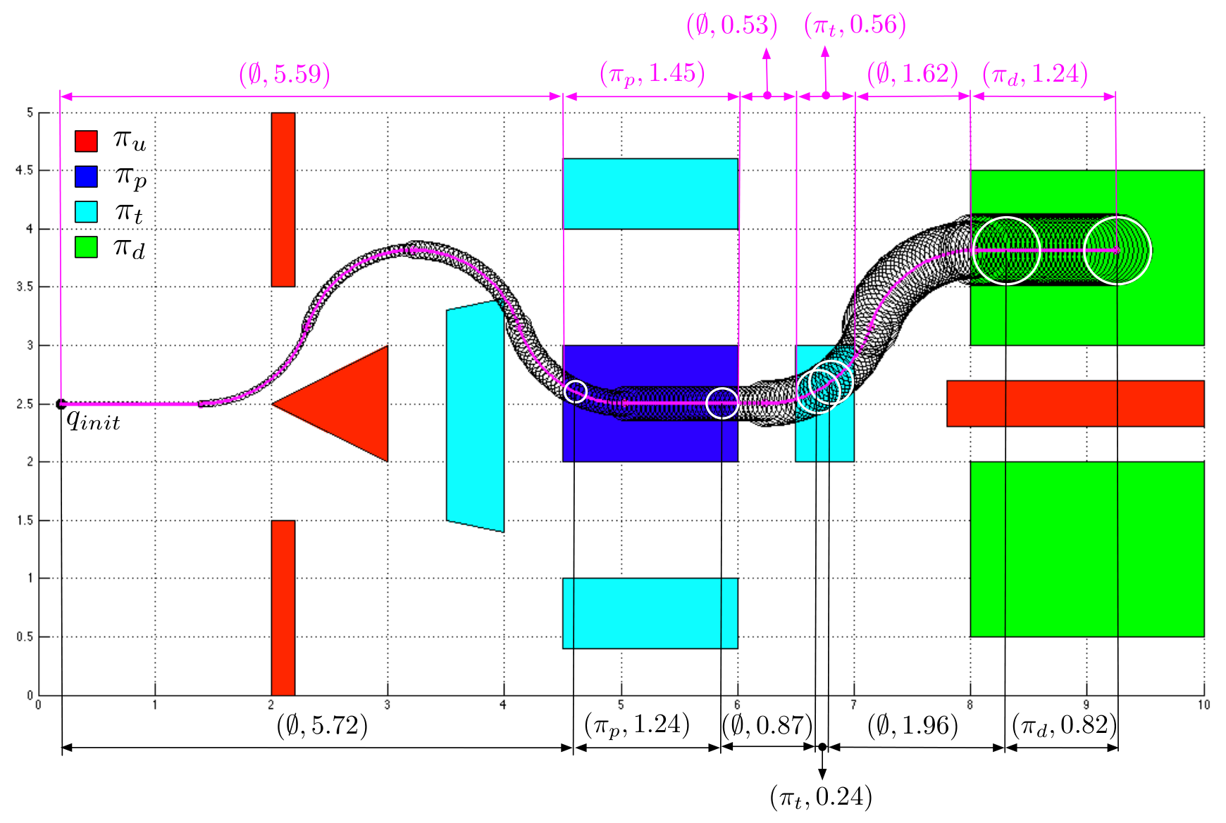
Consider the environment shown in Fig. 2. Let , where label the unsafe, pick-up, test and the drop-off regions, respectively. Let the motion specification be as follows:
Start from an initial state and reach a pick-up region within time units to pick up a load. After entering the pick-up region reach a test region within time units and stay in it at least time units. Finally, after entering the test region reach a drop-off region within time units to drop off the load. Always avoid the unsafe regions.
The specification translates to BLTL formula :
| (3) |

We assume that the vehicle can precisely determine its initial state , in a known map of the environment. While the vehicle moves, incremental encoder measurements are available at each stage . We define a vehicle control strategy as a map that takes as input a sequence of pairs of measured intervals , and returns control inputs and at stage . We are ready to formulate the main problem we consider in this paper:
Problem 1
To fully specify Problem 1, we need to define the satisfaction of a BLTL formula by a trajectory of the system from Eqn. (1). Formal definition is given in Sec. IV. Informally, produces a finite trace , , , , where is the satisfied proposition22 2 Since the regions of interest are non-overlapping it follows that . and is the time spent satisfying , as time evolves. A trajectory satisfies BLTL formula if and only if the generated trace satisfies the formula. Given , for the duration of the motion we use the smallest for which model checking a trace is well defined, i.e., the smallest for which the maximum nested sum of time bounds (see [ZPC10]) is at most .
III-B Approach
In this paper, we develop a suboptimal solution to Problem 1 consisting of three steps. First, we define a finite state MDP that captures every sequence realization of pairs of measurements returned by the incremental encoders. States of the MDP correspond to the sequences of pairs of measured intervals and the actions correspond to the control inputs.
Second, we find a control policy for the MDP that maximizes the probability of satisfying BLTL formula . Because of the size of the MDP, finding the exact solution is computationally too expensive. We decided to trade-off correctness for scalability and we use computationally efficient technique based on system sampling. We use recent results in SMC for MDPs ([HMZ+12]) to obtain an MDP control policy and BIE algorithm ([ZPC10]) to estimate the probability of satisfying .
Finally, since each state of the MDP corresponds to a unique sequence of pairs of measured intervals, we translate the control policy to a vehicle control strategy. In addition, we show that the probability of satisfying , in the original environment, is bounded from below by the probability of satisfying the specification on the MDP under the obtained control policy.
IV Generating a trace
In this section we explain how, given a state trajectory the corresponding trace is generated. Let us denote as the set of positions that satisfy proposition , where is the set of regions labeled with proposition .
Definition 3 (Generating a trace)
The trace corresponding to a state trajectory is a finite sequence , , , , , where is the satisfied proposition and is the time spent satisfying , generated according to the following rules, for all :
iff and otherwise.
Let be the satisfied proposition at some . Then:
- 1.
If , then , iff (i) s.t. , and (ii) s.t. , and , with .
- 2.
If , then iff s.t. , and , with .
Let for , be the current satisfied propositions. Then, .
A trajectory satisfies BLTL formula (Eqn. (2)) if and only if the trace generated according to the rules stated above satisfies the formula. Note that, since the duration of the motion is finite, the generated trace is also finite. In [ZPC10] the authors show that BLTL requires only traces of bounded lengths. The fact that the trace satisfies is denoted . Given a trace , the -th state of , denoted , is , . We denote as the finite subsequence of that starts in . Finally, given a formula , we denote subformula as , . Using the BLTL semantics one can derive the following conditions to determine whether :
Definition 4 (Satisfaction conditions)
Given a trace and a BLTL formula (Eqn. (2)), let for , be such that for some the following holds:
- 1.
,
- 2.
for each , ,
- 3.
, and
- 4.
.
Then, . If , s.t. where with , then .
Example 2
Consider the environment and the sample state (position) trajectory shown in Fig. . Let be as in Eq. (3) with the following numerical values for the time bounds: , , , and . The trajectory generates trace . The following holds: since for and , , , ; since for and , , , and ; and since for and , , and ; Thus, .
V Construction of an MDP Model
Recall that is a random variable with a continuous probability density function supported on the bounded interval , . The probability density functions are obtained through experimental trials (see Sec. IX) and they are defined as follows:
| (4) |
, , s.t. , .
An MDP that captures every sequence realization of pairs of measurements returned by the incremental encoders is defined as a tuple , where:
- •
. The meaning of the state is as follows: , means that at stage , , the pair of measured intervals is .
- •
is the initial state.
- •
is the set of actions, where is a dummy action.
- •
gives the enabled actions at state : if , i.e., if the termination time is reached, , otherwise .
- •
is a transition probability function constructed by the following rules:
- 1.
If then iff and where , and ;
- 2.
If then iff and ;
- 3.
otherwise.
- 1.
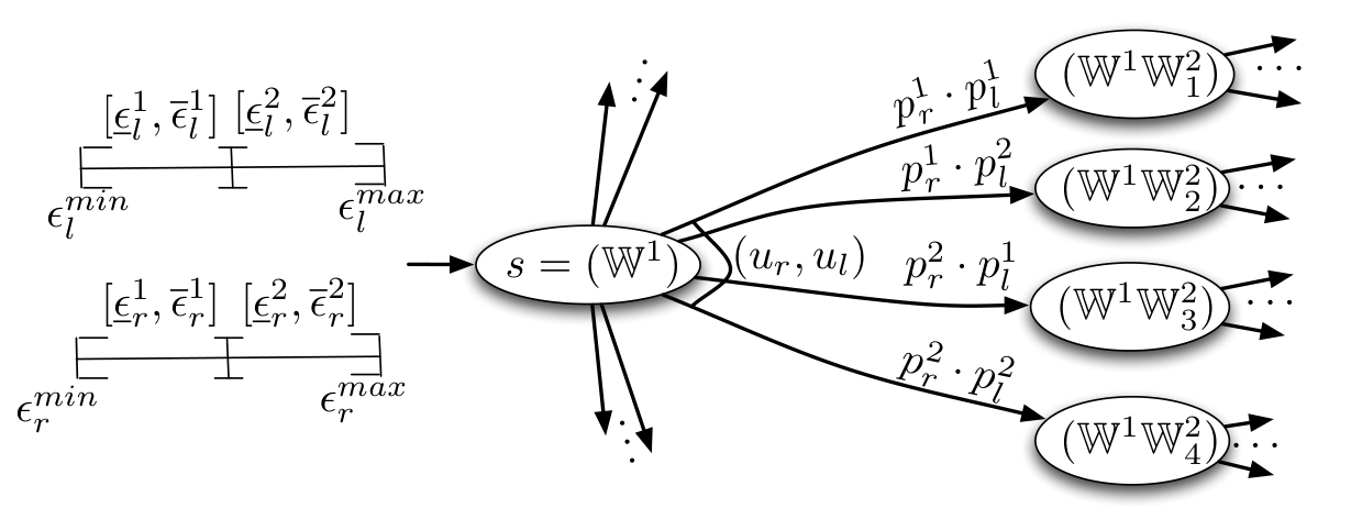
Rule 1) defined above follows from the fact that given and as the control inputs at stage , the pair of measured intervals at stage is with probability , since and , which follows from Eqn. (4) (see the MDP fragment in Fig. 3). Rule 2) states that if the length of is equal to , i.e., if the termination time is reached, then with
Proposition 1
The model defined above is a valid MDP, i.e., it satisfies the Markov property and is a transition probability function.
Proof: The proof follows from construction of . Given current state and an action , the conditional probability distribution of future states depends only on the current state , not on the sequences of events that preceded it (see rule 1) above). Thus, the Markov property holds. In addition, since for every and : , it follows that is a valid transition probability function.
VI Position uncertainty
VI-A Nominal state trajectory
For each interval belonging to the set of noise intervals , we define a representative value , , , i.e., is the midpoint of interval , . We denote the set of representative values as , .
We use , and , , , to denote the state trajectory and the constant applied controls at stage , respectively. With a slight abuse of notation, we use to denote the end of state trajectory , i.e., . Given state , the state trajectory can be derived by integrating the system given by Eqn. (1) from the initial state , and taking into account the applied controls are constant and equal to and . Throughout the paper, we will also denote this trajectory by , when we want to explicitly capture the initial state and the constant applied controls and .
Given a path through the MDP:
| (5) |
where , with , , we define the nominal state trajectory , , as follows:
, where is such that , and . For every path through the MDP, its nominal state trajectory is well defined. The next step is to define the uncertainty evolution, along the nominal state trajectory, since the applied controls can take any value within the measured intervals.
VI-B Position uncertainty evolution
Since a motion specification is a statement about the propositions satisfied by the regions of interest in the environment, in order to answer whether some state trajectory satisfies BLTL formula it is sufficient to know its projection in . Therefore, we focus only on the position uncertainty.
The position uncertainty of the vehicle when its nominal position is is modeled as a disc centered at with radius , where denotes the distance uncertainty:
| (6) |
where denotes the Euclidian distance. Next, we explain how to obtain .
First, let denote the orientation uncertainty. Let , , be the nominal state trajectory corresponding to a path through the MDP (Eqn. (5)). Then, can be partitioned into state trajectories: , , , where is such that , and (see Fig. 4). The distance and orientation uncertainty at state are denoted as and , respectively. We set and at state equal to:
| (7) |
where
| (8) |
for , where and .

Eqn. (7) and (8) are obtained using a worst scenario assumption. At stage , the pair of measured intervals is and we use the endpoints of the measured intervals to define set . is the smallest set of points in , at the end of stage , guaranteed to contain (i) the state with the maximum distance (in Euclidian sense) from given that the applied controls at stage are within the measured intervals at stage , and (ii) the state with the maximum orientation difference compared to given that the applied controls at stage are within the measured intervals at stage , . (for more details about see [FMAG98]). An example is given in Fig. 4.
From Eqn. (7) and (8) it follows that, given a nominal state trajectory , , the distance uncertainty increases as a function of time. The way it changes along makes it difficult to characterize the exact shape of the position uncertainty region. Instead, we use a conservative approximation of the region. We define as an approximate distance uncertainty trajectory and we set , , , i.e., we set the distance uncertainty along the state trajectory equal to the maximum value of the distance uncertainty along , which is at state . An example illustrating this idea is given in Fig. 4.
Proposition 2
Given a path through the MDP (Eqn. (5)), and the corresponding and , , as defined above, then any state trajectory , , , where , and , is within the uncertainty region, i.e., , .
VII Generating a trace under the position uncertainty
Let be a nominal state trajectory with the distance uncertainty trajectory , . In this subsection we introduce a set of conservative rules according to which the trace corresponding to the uncertainty region is generated. This rules guarantee that if the generated trace satisfies (Eqn. (2)) then any state (position) trajectory, inside , will satisfy .
Definition 5 (Generating a trace under uncertainty)
The trace corresponding to an uncertainty region is a finite sequence , , , , , where is the satisfied proposition and is the time spent satisfying , generated according to the following rules, for all :
iff , iff and otherwise.
Let be the satisfied proposition at some . Then:
- 1.
If , then iff s.t. and , with .
- 2.
If , then iff s.t. and , with .
- 3.
If , then , iff
- (a)
s.t. ,
- (b)
s.t. ,
- (c)
s.t.
and , with .
- (a)
- 4.
If , then , iff
- (a)
s.t. ,
- (b)
s.t. , , and
and , with .
- (a)
Let for , be the current satisfied proposition. Then .
In Fig. 5 we show an uncertainty region and the corresponding trace generated according to rules stated above. Next, we show that if the trace corresponding to an uncertainty region satisfies , then any state (position) trajectory inside the uncertainty region also satisfies .
Proposition 3
Proof: First, we state two relations between the given traces:
- 1.
Let for some . Then, the following holds: such that and .
Informally, if is the time spent inside the region satisfying proposition , then will spend at least time units inside that region. - 2.
Let and for some , . Then, the following holds: , such that and . In addition, .
Informally, if the time between entering a region satisfying and then entering a region satisfying is time units, then the time between entering the region satisfying and then entering the region satisfying is bounded from above by . For more intuition about this relations see Fig. 5.
VIII Vehicle Control Strategy
Given the MDP , the next step is to obtain a control policy that maximizes the probability of generating a path through such that the corresponding trace (as defined in Sec. VI and VII) is satisfying. There are existing approaches that, given an MDP and a temporal logic formula, generate an exact control policy that maximizes the probability of satisfying the specification. In general, exact techniques rely on reasoning about the entire state space, which is a limiting factor in their applicability to large problems. Given , , , and , the size of the MDP is bounded above by . Even for a simple case study, due to the size of , using the exact methods to obtain a control policy is computationally too expensive. Therefore, we decide to trade-off correctness for scalability and use computationally efficient techniques based on system sampling.
VIII-A Overview
We obtain a suboptimal control policy by iterating over the control synthesis and the probability estimation procedure until the stopping criterion is met (see Sec. VIII-C). In the control synthesis procedure we use the control synthesis approach from [HMZ+12] to generate a control policy for the MDP . In particular we use a control policy optimization part of the algorithm which consists of the control policy evaluation and the control policy improvement procedure to incrementally improve a candidate control policy (control policy is initialized with a uniform distribution at each state). Next, in the probability estimation procedure we use SMC by BIE, as presented in [ZPC10]. We estimate the probability that the MDP , under the candidate control policy, generates a path such that the corresponding trace satisfies BLTL formula . Finally, if the estimated probability converges, i.e., if the stopping criterion is met, we map the control policy to a vehicle control strategy. Otherwise, the control synthesis procedure is restarted using the latest update of the control policy. The flow of this approach is depicted in Fig. 6.

VIII-B Control synthesis
The details of the control policy optimization algorithm can be found in [HMZ+12] and here we only give an informal overview of the approach. In the control policy evaluation procedure we sample paths of the MDP under the current control policy . Given a path , where , the corresponding trace is generated as described in Sec. VI and VII. Next, we check formula on each and estimate how likely it is for each action to lead to the satisfaction of BLTL formula , i.e., we obtain the estimate of the probability that a path crossing a state-action pair, , , in will generate a trace that satisfies . These estimates are then used in the control policy improvement procedure, in which we update the control policy by reinforcing the actions that led to the satisfaction of most often. The authors ([HMZ+12]) show that the updated control policy is provably better than the previous one by focusing on more promising regions of the state space.
The algorithm takes as input MDP , BLTL formula and the current control policy , together with the parameters of the algorithm (a greediness parameter , a history parameter , and the number of sample paths in control policy evaluation procedure, denoted by ), and returns the updated probabilistic control policy . In the next step, to estimate the probability of satisfaction, we use the deterministic version of , denoted where: for all and ,
In words, we compute a control policy that always picks the best estimated action at each state.
VIII-C Probability estimation
Next, we determine the estimate of the probability that the MDP , under the deterministic control policy , generates a path such that the corresponding trace satisfies BLTL formula . To do so we use the BIE algorithm as presented in [ZPC10]. We denote the exact probability as and the estimate as .
The inputs of the algorithm are the MDP , control policy , BLTL formula , half interval size , interval coefficient , and the coefficients of the Beta prior. The algorithm returns . The algorithm generates traces by sampling paths through under (as described in Sec. VI and VII) and checks whether the corresponding traces satisfy , until enough statistical evidence has been found to support the claim that is inside the interval with arbitrarily high probability, i.e., .
We stop iterating over the control synthesis and the probability estimation procedure when the difference between the two consecutive probability estimates converges to a neighborhood of radius , i.e., when the difference is smaller or equal to . Let and be the current control policy and the corresponding probability estimate, respectively, when the stopping criterion is met.
VIII-D Control strategy
The vehicle control strategy is a function that maps a sequence of pairs of measured intervals, i.e., a state of the MDP, to the control inputs:
| (9) |
with .
At stage , the control inputs are
Thus, given a sequence of pairs of measured intervals, returns the control inputs for the next stage; the control inputs are equal to the action returned by at the state of the MDP corresponding to that sequence.
Theorem 1
The probability that the system given by Eqn. (1), under the vehicle control strategy , generates a state trajectory that satisfies BLTL formula (Eqn. (2)) is bounded from below by , where .
Proof: Let be a path through the MDP and the corresponding uncertainty region as defined in Sec. VI. Let be any state trajectory as defined in Prop. 2. Also, let and be the corresponding traces. Trace can (i) satisfy and (ii) not satisfy .
Let us first consider the former. If from Prop. 3 it follows that . Under the probability of generating is equivalent to generating path under . Since under the probability that a path through the MDP generates a satisfying trace is it follows that the probability that the system given by Eqn. (1), under , will generate a satisfying state trajectory is also .
To show that is the lower bound we need to consider the latter case. It is sufficient to observe that because of the conservative approximation of it is possible that satisfies , even though does not satisfy it. Therefore, it follows that the probability that system given by Eqn. (1), under the vehicle control strategy , generates a state trajectory that satisfies BLTL formula , is bounded from below by . The rest of the proof, i.e., , is given in [ZPC10].
VIII-E Complexity
As stated above, the size of the MDP is bounded above by . Obviously, it can be expensive (in sense of memory usage) to store the whole MDP. Since our approach is sample-based, it is not necessary for the MDP to be constructed explicitly. Instead, a state of the MDP is stored only if it is sampled during the control synthesis procedure. As a result, during the execution, the number of states stored in the memory is bounded above by , where is the number of iterations between the control synthesis and the probability estimation procedures.
IX Case study
We considered the system given by Eqn. (1) and we used the numerical values corresponding to Dr. Robot’s x80Pro mobile robot equipped with two incremental encoders. The parameters were m and m. To reduce the complexity, was limited to , where the pairs of control inputs corresponded to a vehicle turning left at , going straight, and turning right at , respectively, when the forward speed is .
Measurement resolution: To obtain the angular wheel velocity, the frequency counting method [PTPZ07] was used, i.e., the encoder pulses inside a given sampling period were counted. The number of pulses per revolution (i.e., the number of windows in the code track of the encoders) was and the sampling period was set to s. Thus, according to [PTPZ07] the measurement resolution was .
Probability density functions: We obtained the distributions through experimental trials. Specifically, we used control inputs from as the robot inputs and then measured the actual angular wheel velocities using the encoders. We obtained () by taking the minimum (maximum) over (), where , , , was the noise interval, of length , determined from the -th measurement of the encoder and was the total number of measurements. Note that , . Finally, the probabilities for Eq. (4) that defined the probability density functions, were equal to the number of times a particular noise interval was measured over . For (i.e., by using each control input from times) we obtained and the corresponding probabilities.
The set of propositions was where labeled the unsafe, pick-up, test1, test2 and the drop-off regions, respectively. The motion specification was:
Start from an initial state and reach a pick-up region within time units and stay in it at least time units, to pick-up the load. After entering the pick-up region, reach a test1 region within time units and stay in it at least time units or reach a test2 region within time units and stay in it at least time units. Finally, after entering the test1 region or the test2 region reach a drop-off region within time units to drop off the load. Always avoid the unsafe regions.
The specification translates to BLTL formula :
| (10) |
Two different environments are shown in Fig. 7. The estimated probability corresponding to environment and was and , respectively. From Eq. (10) it followed that . The numerical values in the control synthesis procedure and the probability estimation procedure were as follows: , , , , , , and . For both environments, we found the vehicle control strategy through the method described in Sec. VIII.

Since it is not possible to obtain the exact probability that the system given by Eqn. (1), under the vehicle control strategy, generates a satisfying state trajectory, in order to verify our result (Theorem 1), we performed multiple runs of BIE algorithm by simulating the system under the vehicle control strategy (using the same numerical values as stated above and by generating traces as described in Sec. IV). We denote the resulting probability estimate as and we compare it to .
| Environment | ||||
|---|---|---|---|---|
| Run 1 | Run 2 | Run 3 | ||
In Fig. 7 we show sample state trajectories and in Table I we compare the estimated probabilities obtained on the MDP, , with the estimated probabilities obtained by simulating the system, . The results support Theorem 1, since is bounded from below by . The discrepancy in the probabilities is mostly due to the conservative approximation of the uncertainty region in Sec. VI. The Matlab code used to obtain the vehicle control strategy ran for approximately 2.2 hours on a computer with a 2.5GHz dual processor.
In Fig. 8 we show a sample run of the robot in environment . A projector was used to display the environment and the state (position) trajectory was reconstructed using the OptiTrack (http://www.naturalpoint.com/optitrack) system with eight cameras.

X Discussion
We developed a feedback control strategy for a stochastic differential drive mobile robot such that the probability of satisfying a time constrained specification given in terms of a temporal logic statement is maximized. By mapping sensor measurements to a Markov Decision Process (MDP) we translate the problem to finding a control policy maximizing the probability of satisfying a Bounded Linear Temporal Logic (BLTL) formula on the MDP. The solution is based on Statistical Model Checking for MDPs and we show that the probability that the vehicle satisfies the specification is bounded from below by the probability of satisfying the specification on the MDP.
The key limitation of the proposed approach is the computation time. Since our algorithm is based on Statistical Model Checking for MDPs presented in [HMZ+12], to put the running time of our algorithm into perspective, we compare it to the running time of Statistical Model Checking for MDPs when dealing with the following motion planning study: each of the two robots living in a grid world must pick up some object and then meet with the other robot within a certain time bound, while avoiding unsafe grids. At each point in time, either robot can try to move 10 grid units in any of the four cardinal directions, but each time a robot moves, it has some probability of ending up somewhere in a radius of grid units of the intended destination. Statistical Model Checking for MDPs (when ) solves this problem in approximately minutes. Now, let us consider the algorithm and the case study presented in this paper. First, note that in order for Theorem 1 to hold, when generating a trace corresponding to an uncertainty region, we have to perform a computationally expensive step of taking the intersection between the uncertainty region and all of the regions of interest (see Def. 5, Sec. VII). Second, note that we are dealing with a system that is continuous both in space and time. Therefore, at each time step, when constructing an uncertainty region, the algorithm is required to perform multiple integrations of the system. Thus, the increase in the computational complexity, in order to have probabilistic guarantees for the original system, is the reason the running time of our algorithm (when ) is approximately hours.
Since sampling (i.e., generating traces) accounts for the majority of our runtime, future work includes improving the sampling performance and making the implementation fully parallel. Additionally, to address the problem of discrepancy between the probabilities obtained on the MDP and the probabilities obtained by simulating the system the future work also includes developing a less conservative uncertainty model.
XI Acknowledgements
The authors gratefully acknowledge David Henriques from Carnegie Mellon University for comments on an earlier draft. Also, the authors would like to thank Benjamin Troxler, Michael Marrazzo and Matt Buckley from Boston University for their help with the experiments.
References
- [ADBS08] A. Abate, A. D’Innocenzo, Maria D. Di Benedetto, and S. Shankar Sastry. Markov Set-Chains as Abstractions of Stochastic Hybrid Systems, volume 1. Springer Verlag, 2008.
- [BK08] C. Baier and J. P. Katoen. Principles of Model Checking. MIT Press, 2008.
- [BM00] D. Balkcom and M. T. Mason. Time Optimal Trajectories for Bounded Velocity Differential Drive Robots. In IEEE International Conference on Robotics and Automation (ICRA) 2000, volume 3, pages 2499 – 2504, 2000.
- [BMKV11] A. Bhatia, M. R. Maly, L. E. Kavraki, and M. Y. Vardi. Motion Planning with Complex Goals. Robotics Automation Magazine, IEEE, 18(3):55 –64, September 2011.
- [CB12] I. Cizelj and C. Belta. Probabilistically Safe Control of Noisy Dubins Vehicles. In International Conference on Intelligent Robots and Systems (IROS) 2012, October 2012.
- [CGP99] E. Clarke, O. Grumberg, and D. A. Peled. Model Checking. The MIT Press, 1999.
- [DABS08] A. D’Innocenzo, A. Abate, M. D. Di Benedetto, and S. Shankar Sastry. Approximate Abstractions of Discrete-Time Controlled Stochastic Hybrid Systems. In IEEE Conf. on Decision and Control, December 2008.
- [DLB12] X. C. Ding, M. Lazar, and C. Belta. Receding Horizon Temporal Logic Control for Finite Deterministic Systems. In American Control Conference (ACC) 2012., June 2012.
- [FMAG98] T. Fraichard, R. Mermond, and R. Alpes-Gravir. Path Planning with Uncertainty for Car-Like Robots. In IEEE International Conference on Robotics and Automation (ICRA) 1998, pages 27–32, 1998.
- [Gir07] A. Girard. Approximately Bisimilar Finite Abstractions of Stable Linear Systems. In International Conference on Hybrid Systems: Computation and Control (HSCC) 2007, pages 231–244, Berlin, Heidelberg, 2007. Springer-Verlag.
- [HMZ+12] D. Henriques, J. Martins, P. Zuliani, A. Platzer, and E. M. Clarke. Statistical Model Checking for Markov Decision Processes. In 9th International Conference on Quantitative Evaluation of SysTems (QEST) 2012, September 2012.
- [JCL+09] S. Kumar Jha, E. M. Clarke, C. J. Langmead, A. Legay, A. Platzer, and P. Zuliani. A Bayesian Approach to Model Checking Biological Systems. In International Conference on Computational Methods in Systems Biology (CMSB) 2009, pages 218–234, 2009.
- [JP09] A. A. Julius and G. J. Pappas. Approximations of Stochastic Hybrid Systems. IEEE Transactions on Automatic Control, 54(6):1193 –1203, 2009.
- [KB08a] M. Kloetzer and C. Belta. Dealing with Non-Determinism in Symbolic Control. In Hybrid Systems: Computation and Control: 11th International Workshop, Lecture Notes in Computer Science, pages 287–300. Springer Berlin / Heidelberg, 2008.
- [KB08b] M. Kloetzer and C. Belta. A Fully Automated Framework for Control of Linear Systems from Temporal Logic Specifications. IEEE Transactions on Automatic Control, 53(1):287 –297, 2008.
- [KF08] S. Karaman and E. Frazzoli. Vehicle Routing Problem with Metric Temporal Logic Specifications. In IEEE Conference on Decision and Control (CDC) 2008., pages 3953 –3958, 2008.
- [KGFP07] H. Kress-Gazit, G. E. Fainekos, and G. J. Pappas. Where’s Waldo? Sensor-Based Temporal Logic Motion Planning. In IEEE International Conference on Robotics and Automation (ICRA) 2007, pages 3116–3121, 2007.
- [LAB12] M. Lahijanian, S. B. Andersson, and C. Belta. Temporal Logic Motion Planning and Control With Probabilistic Satisfaction Guarantees. IEEE Transactions on Robotics, 28(2):396 –409, 2012.
- [LaV06] S. M. LaValle. Planning Algorithms. Cambridge University Press, Cambridge, U.K., 2006.
- [LK04] S. G. Loizou and K. J. Kyriakopoulos. Automatic Synthesis of Multi-Agent Motion Tasks Based on LTL specifications. In Decision and Control, 2004. CDC. 43rd IEEE Conference on, volume 1, pages 153 – 158 Vol.1, Dec. 2004.
- [PTPZ07] R. Petrella, M. Tursini, L. Peretti, and M. Zigliotto. Speed Measurement Algorithms for Low-Resolution Incremental Encoder Equipped Drives: A Comparative Analysis. In International Aegean Conference on Electrical Machines and Power Electronics (ACEMP) 2007, pages 780 –787, 2007.
- [TP06] P. Tabuada and G. J. Pappas. Linear Time Logic Control of Discrete-Time Linear Systems. IEEE Transactions on Automatic Control, 51(12):1862 –1877, 2006.
- [WTM09] T. Wongpiromsarn, U. Topcu, and R. M. Murray. Receding Horizon Temporal Logic Planning for Dynamical Systems. In 48th IEEE Conference on Decision and Control (CDC) 2009, pages 5997 –6004, 2009.
- [YTC+12] B. Yordanov, J. Tumova, I. Cerna, J. Barnat, and C. Belta. Temporal Logic Control of Discrete-Time Piecewise Affine Systems. IEEE Transactions on Automatic Control, 57(6):1491 –1504, 2012.
- [ZPC10] P. Zuliani, A. Platzer, and E. M. Clarke. Bayesian Statistical Model Checking with Application to Simulink/Stateflow Verification. In International Conference on Hybrid systems: Computation and Control (HSCC) 2010, pages 243–252, 2010.