Dynamics of waves in 1D electron systems:
Density oscillations
driven by population inversion
Abstract
We explore dynamics of a density pulse induced by a local quench in a one-dimensional electron system. The spectral curvature leads to an “overturn” (population inversion) of the wave. We show that beyond this time the density profile develops strong oscillations with a period much larger than the Fermi wave length. The effect is studied first for the case of free fermions by means of direct quantum simulations and via semiclassical analysis of the evolution of Wigner function. We demonstrate then that the period of oscillations is correctly reproduced by a hydrodynamic theory with an appropriate dispersive term. Finally, we explore the effect of different types of electron-electron interaction on the phenomenon. We show that sufficiently strong interaction [ where is the fermionic mass and the relevant spatial scale] determines the dominant dispersive term in the hydrodynamic equations. Hydrodynamic theory reveals crucial dependence of the density evolution on the relative sign of the interaction and the density perturbation.
pacs
73.23.-b, 73.21.Hb, 71.10.PmI Introduction
Transport properties of interacting one-dimensional (1D) systems keep attracting a great deal of research interest. Experimental realizations of 1D fermionic systems include, in particular, carbon nanotubes, semiconductor and metallic nanowires, as well as quantum Hall (and other topological insulator) edges. Further, 1D bosonic and fermionic systems can be engineered by using cold atomic gases in optical traps of the corresponding geometry. A standard and powerful theoretical approach to interacting 1D systems is the bosonization [1, 2, 3, 4, 5]. When (i) the spectrum is linearized, (ii) backscattering processes are neglected, and (iii) the physics near equilibrium is explored, the bosonization reduces the original interacting problem to a Gaussian field theory, thus reducing evaluation of physical observables to a straightforward calculation of Gaussian integrals. When one (or several) of the above three conditions is not fulfilled, the theoretical analysis becomes much more involved. In the present paper we will focus on non-equilibrium physics of 1D fermionic systems in the regime where the spectral curvature is of crucial importance.
Properties of 1D interacting systems with spectral nonlinearity have been addressed in a series of recent theoretical works[6, 7, 8, 9, 10]. Here we will consider the time evolution of a density pulse created by a local quench in a 1D fermionic system (that will be assumed to be spinless or spin-polarized for simplicity). We will assume that this pulse is quasiclassical (i.e., has a characteristic spatial extension much larger than the Fermi wave length) and sufficiently strong (i.e., contains a large number of electrons). For not too long times the evolution seems to be fully harmless: the pulse splits into left- and right-moving parts that separate and move away from each other, approximately preserving theirs shape. They key point is that the shape would remain strictly unchanged only for linear dispersion of excitations, while the non-linearity of dispersion leads to a deformation of the pulse. As a result, at a certain finite time the pulse tends to “overturn”. The problem to be addressed is what happens with the density profile beyond this time.
The above problem was formulated in Ref. 11 in the context of Calogero model that was argued to describe the fractional quantum Hall (FQH) edges (see also a recent paper Ref. 12). Using quantum hydrodynamics approach, the authors of Refs. 11, 12 came to a conclusion that a density pulse formed in a FQH edge will evolve in a sequence of well separated solitons with a quantized charge (equal to for Laughlin states).
In the present work we perform a systematic analysis of the pulse dynamics for free fermions as well for those with different types of interaction. We begin by considering a non-interacting case (Sec. II). Quantum simulations show development of density oscillations at sufficiently large times. By analyzing evolution of the Wigner function, we show that once the semiclassical phase-space distribution overturns (i.e. develops a population inversion characterized by three “Fermi momenta”), strong oscillations of density are generated in the corresponding region of space. The characteristic scale of these oscillations is much larger than the Fermi wave length . The oscillations can be understood as Friedel oscillations between different Fermi-momentum branches.
In Sec. III we switch to the bosonization language and discuss a connection between free-fermion oscillations studied in Sec. II and classical hydrodynamics. In the latter class of problems [13] oscillating structures are known to develop when shock waves are regularized by dispersive terms. We show that although dispersive terms arise already within Haldane bosonization formalism of free fermions with curvature, the dominant terms should come from summing the loop expansion. While we do not know how to take into account these effects systematically, we approximate them by including in the classical hydrodynamic equation a term corresponding to an upper (for a positive pulse) branch of the particle-hole continuum. Solving the corresponding equation (which is of Benjamin-Ono type), we show that it yields oscillations with correct period (including its spatial variation) but with an amplitude several times larger than the right one. This shows that the above classical hydrodynamic equation does catch some important physics of the developing “dispersive shock” of a free-fermion pulse but does not represent a fully controllable approximation.
Section IV is devoted to an analysis of the interaction effects on the pulse evolution. We consider first the case of a short-range interaction and argue that the discovered oscillations remain largely preserved, up to two modifications: (i) conventional Luttinger-liquid renormalization of the Fermi velocity, and (ii) washing out of oscillations at long times due to inelastic processes. We turn then to the case of a long-range interaction. We show that when the interaction decays sufficiently slowly (specifically, at large distances , and is a electronic mass), the leading contribution to the dispersion results from the interaction term, and the problem can be treated quasiclassically (i.e. loops can be neglected), giving rise to a classical hydrodynamic equation. The evolution of the pulse according to such an equation depends crucially on the sign of the pulse and the sign of the interaction (or, more precisely, on the relative sign between them). When the interaction is repulsive and the density pulse is downward, oscillations develop similarly to the case of free fermions (or short-range interaction). The period of oscillations gets however parametrically larger. On the other hand, for an upward pulse (and still assuming a repulsive long-range interaction), the pulse splits in a sequence of “solitons” (whose charge is in general not quantized, except for the case of interaction).
Section V contains a summary of our results and a discussion of prospective research directions.
II Free fermions


In this section and in Sec. III we study the evolution of a “quasiclassical” density disturbance of the Fermi sea of free fermions. We begin (Sec. II.1) by formulating the problem and performing its numerical modelling which shows emergence of density oscillations after the time corresponding to overturning of the initial packet. In Sec. II.2 we solve this problem analytically by using the straightforward (“fermionic”) approach. Specifically, we demonstrate that, once the dispersion induces a population inversion within the pulse, phase-space oscillation of the Wigner function give rise to density oscillations. Analyzing the resulting density oscillations, we find a perfect agreement with the results of numerical simulations of Sec. II.1. Finally, in Sec. III we make a link to “dispersive shocks” in the classical hydrodynamics. We show that when the dispersive term corresponding to the appropriate branch of the particle-hole spectrum is incorporated into classical hydrodynamic equations, the latter reproduce correctly the period of emerging oscillations (but considerably overestimates their amplitude).
II.1 Formulation of the problem and numerical simulations


The problem that we address is formulated in a rather simple way. We assume that a non-uniform fermionic density was created by application of a smooth (on the scale of ) and relatively weak (compared to the Fermi energy ) external potential to the unperturbed Fermi sea (Fig. 1). The system at is in its ground state characterized by the fermionic density
| (1) |
Here, is the Fermi momentum at infinity. Note that all the corrections to the semi-classical result (1) are exponentially small as long as is smooth on the scale of . For transparency of discussion we assume that the density pulse has a shape of a single hump (as shown schematically in Fig. 1), i.e. that and has a single minimum at .
At the potential is suddenly switched off, which results in the appearance of a non-equilibrium state and subsequent propagation of the density perturbation created by . Our goal will be to explore this density evolution at sufficiently long times. We will assume that the number of particles within the initial pulse is large, , where and are the characteristic extension of the pulse and its amplitude, respectively. The interesting physics will emerge at times , when the semiclassical phase-space distribution overturns.
Since the fermions are free and their state was prepared in the coherent manner described above, the full information on the quantum state of the system is encoded in the Wigner function
| (2) | |||
satisfying at the (exact!) Boltzmann equation
| (3) |
In this equation we have set the particle mass to unity. Let us note that the mass will enter our results only through the overall time scale. Thus, dependence on can be eliminated completely by measuring in units of .
Equation (3) is trivially solved, yielding
| (4) |
Therefore, once we know the Wigner function of the initial () state, the Wigner function of the evolved () state can be immediately obtained.
Let us examine now the Wigner function of the initial state. Semiclassically one would expect that takes value unity for the occupied electronic states that are below the position-dependent Fermi momentum and is zero for empty ones (above ):
| (5) |
In this approximation, the time-dependent state of the fermions after the quench (i.e. at ) is fully characterized by the Fermi surface separating occupied and unoccupied single-particle states in the phase space and satisfying the Euler equation (we concentrate on the Fermi surface for the right-moving particles with )
| (6) |
While capturing correctly the physics at small times, the Euler equation (6) suffers from the shock-wave phenomenon. Specifically, for arbitrarily smooth initial conditions, the curvature of the electronic dispersion relation , makes the Fermi surface multivalued at large enough times () and leads to the appearance of infinite spatial gradients of fermionic density (Fig. 3, middle and bottom panels). This suggests that the simple semiclassical description (6), (5) may become insufficient beyond the time when the shock occurs, raising the question of what happens with the density profile at .
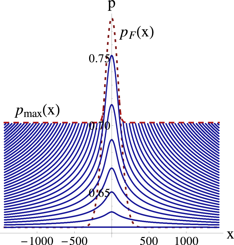
We have performed direct quantum simulations of this problem by using a tight-binding free-fermion model. Figure 2 demonstrates the density evolution from initial state at (left panel) to state at certain time after the shock (approximately five times larger than ). At only the right-moving part of the density pulse is shown. A full movie of density evolution is available online [14]. The initial density perturbation was Gaussian
| (7) |
with dispersion of about lattice sites and contained electrons. The density of the underlying Fermi sea is fermion per site, so that the cosine-shaped dispersion relation of the tight-binding model can be well approximated by a parabola.
For convenience of the reader the snapshot of the density at is also shown in the top panel of Fig. 3. Comparing the exact quantum result (Fig.3, top) to the naive semiclassical result dictated by the Euler equation (Fig. 3, bottom), we see that the shock gets regularized via the onset of pronounced density oscillations at the front edge of the pulse. It is important to emphasize that the period of those oscillations is controlled by the amplitude of the density perturbation and is thus much larger than . (We will perform a detailed quantitative analysis of the oscillation period below in Sec. II.2.) From this point of view, the developing oscillations may be considered as quasiclassical: their characteristic scale is much larger than . Thus, a smooth initial density stays smooth at scale also at times after the “shock”.
We thus face an apparent contradiction: the density profile remains “quasiclassical” (smooth on the scale of ) after the shock but develops strong oscillations that are not caught by the quasiclassical approximation based on Eqs. (6), (5). The resolution of this “paradox” is related to the fact that Eq. (5) is not the fully correct semiclassical (in the above sense) approximation for the Wigner function of fermions in a smooth potential well. As was pointed out in Ref. 15, instead of having abrupt drop from to at Fermi momentum, as a function of develops oscillations near . Those oscillations can be considered as a semiclassical effect in the sense that their form knows nothing about and is controlled solely by the derivatives of . In Sec. II.2 we give a detailed account of the oscillations in the Wigner function and of their implications for the density evolution.
II.2 Wigner function of fermions in a potential well and density oscillations
The Wigner function of the initial state satisfies the equation
| (8) |
where the coordinate is conjugate (in the sense of Fourier transformation) to the momentum , cf. Eq. (2). As we are interested in the behavior of close to one of the Fermi edges we can replace by (we concentrate here on the right Fermi edge). This corresponds to taking the limit while keeping the profile fixed. Solving the resulting equation
| (9) |
with the condition at infinity
| (10) |
and transforming the result to momentum space, we find in agreement with Ref. 15
| (11) | |||
| (12) |
Note that our approach is slightly different from that of Ref. 15: we consider an equilibrium state in a potential , while the authors of Ref. 15 construct a coherent state by acting on the homogeneous Fermi vacuum with an exponential of a bilinear in fermionic operators.
The general structure of the Wigner function can be inferred from Eqs. (11), (12) by performing the integration with making use of the saddle-point method. The saddle-point equation for the action (12)
| (13) |
has no real-valued solutions for or
| (14) |
In these parts of the phase space the integral (11) is controlled by the singularity at , and can be well approximated by Heaviside -function.
On the contrary, for there exist (at least) two solutions to the saddle point equation providing an oscillatory contribution to the Wigner function
| (15) |
Here is the coefficient controlled by the fluctuations around the saddle points. The phase of oscillations is given by . It defines the period of oscillations with the momentum via . Counting the powers of imaginary unit in the saddle point integration one easily finds that the maxima of the Wigner function appear at .
In a sufficiently close vicinity of the local Fermi surface, one can locally approximate by a parabola and express the Wigner function in terms of the Airy function [15]. This approximation is however insufficient for our purposes, as the density oscillations will originate from Wigner function oscillations at all scales .

The oscillatory behavior of is illustrated in Fig. 4 where we plot (calculated via numerical integration of (11)) as a function of momentum. To generate the plot we have assumed the Gaussian density used in the quantum simulations presented in Sec. II.1 and in Fig. 2. A straightforward analysis of the saddle-point equation shows that, upon variation of momentum from to , varies monotonically from to , where
| (16) |
is (generally non-integer) number of particles in the pulse. Accordingly, the Wigner function of Fig. 4 shows oscillations corresponding to approximately right-moving particles. Vertical lines in Fig. 4 mark the momenta satisfying the condition .
The overall behavior of in the phase space can be conveniently represented by lines of constant action . For the case of Gaussian density the corresponding pictures is shown on Fig. 5. The green dashed line here represents the border of the region of developed oscillations. The solid blue lines are the lines of constant action . Finally, the dotted line shows the -dependent Fermi level. The “topology” of the plot can be understood on general grounds and does not depend on the specific density . At large the action is a steep function of momentum and, when taken modulo , acquires any given value many times. Among the lines of constant action coming from , exactly (this denotes the integer part of ) lines cross the -axes and flow to , while other lines end up on the border where the solution to the saddle point equation becomes complex.
Let us now discuss the implications of the above results for the fermionic density which is equal to the integral over momentum of the Wigner function. In the initial state the density is insensitive to the oscillations of the Wigner function. Indeed, one can observe that the contour of momentum integration (vertical line on Fig. 5) crosses many contours of constant but does not touch any of them, so that there is no stationary-point contribution to the integral. In fact, evaluating the integral of Eq. (11), we find that in the considered (large ) approximation the equality is exact.
The evolution of each contour line of the action is governed by the Euler equation (6). The behavior of the Wigner function after the shock, , is illustrated by Fig. 6. Now the vertical lines do touch the contours of constant action. A touching point becomes the saddle point for the integration over momentum and the oscillations in start to contribute to the density. This implies a maximum in the density each time the integration line touches the contour line corresponding to .
The brown curve in the upper part of Fig. 6 shows the density obtained via numerical integration of the Wigner function (11). This is almost indistinguishable from the result of first-principle quantum simulations (top panel of Fig. 3). We observe that the positions of the maxima of the density are in accord with the above argument based on the saddle-point approximation.

One can now determine the period of the density modulations. Let us focus on the region closer to the front edge of the pulse where the oscillations are clearly governed by a single harmonics, see Fig. 3, and are perfectly described by the saddle-point argument as shown in Fig. 6. As this figure further illustrates, the integration contour touches the contour lines near and the period of the density oscillations is set by . In this regime we have
| (17) |
Thus, and we immediately infer the period
| (18) |
It is not difficult to generalize this argument to the region closer to the top of the pulse. Assuming for simplicity that the time that has passed after shock is of the order of the shock time , we find that the characteristic spatial scale for the first few oscillations (just to the right of the maximum of the pulse) is larger than (18) by a factor (for the parameters used in our plots this is approximately two). Some complication comes from the fact that in this region a superposition of oscillations originating from different regions in phase space takes place. Indeed, as is clearly seen in the lower panel of Fig. 6, constant-action contours that do not terminate at may have two points with infinite slope, and each of them will give a stationary-phase contribution when the momentum integration is performed. This superposition explains a somewhat irregular oscillation pattern in the corresponding spatial region.
The obtained oscillations can be interpreted as Friedel-type oscillations between different branches of the Fermi momentum (that becomes multivalued after the “shock”). In particular, in the front region, the upper two branches are close to the maximum value, , while the lower branch is essentially equal to , which yields exactly Eq. (18).
III Hydrodynamics of free fermions
The analysis of the previous section provides a detailed description of the evolution of coherent perturbation in the density of free fermions. The analysis is complete and, as was also confirmed by numerical simulations, essentially exact under our basic assumptions. It is appealing however to try to formulate a hydrodynamic description of the problem which, in contrast to the fermionic approach utilizing the notion of Wigner function, would involve as fundamental objects only the density and the velocity of the electronic fluid. Indeed, the hydrodynamics (bosonization) constitutes a convenient and powerful framework for the discussion of interaction effects (to be considered in Sec. IV below) which are otherwise hard to access.
Usually, hydrodynamics rests on the assumption of local equilibrium forced by the particle collisions which wash out any features in the particle distribution function. In the present problem no such equilibrium exists. Moreover, we saw above that the oscillating behavior of is crucial for the density ripples observed in the shock region. Hence, one can expect that the evolution of the quantum-coherent many-particle state can not be controllably described by classical equations of hydrodynamic type. Despite this fact, one can ask if it is possible to design phenomenological hydrodynamic equations which would capture qualitative features of the true density evolution. In this section we show that this is indeed possible and such phenomenological equations provide important insight into the physics of non-equilibrium many-particle system.
In our search for hydrodynamics it is convenient to start from the Euler equation (6) corresponding to the neglect of all oscillatory features in the Wigner function . Combined with analogous equation for the Fermi surface of left electrons at it can be rephrased in terms of the mean density and velocity of the fluid as
| (19) | |||
| (20) |
Of course, equations (19) suffer from the same shock phenomenon as the original equation (6). Phenomenologically, we would like to add some terms to Eq. (19) regularizing the shock instability. We know that regularization goes trough the onset of density ripples in the shock region. This phenomenon is well known in hydrodynamics and usually referred to as “dispersive regularization”[16]. It takes place when the shock caused by non-linearity gets regularized by higher order derivatives consistent with the time reversal invariance of the equations. The classical examples are the Korteweg-de-Vries (KdV) and Gross-Pitaevskii equations. It is the requirement of time reversal that makes the “dispersive regularization” very different from “dissipative regularization” achieved by the introduction into the system of some type of viscosity. Examples of the latter type are Navier-Stokes and Burgers equations.
Let us now point out that Eqs. (19) appear in the theory of Fermi gas in yet another context and with slightly different meaning. Specifically, the standard bosonization procedure applied to the fermions with quadratic spectrum leads to Hamiltonian [17, 18, 19]
| (21) |
Here, and are operators with the commutation relations
| (22) |
The Hamiltonian and the commutation relations imply the operator equations of motion usually referred to as “quantum Euler equations”
| (23) |
One can now see that there exist two sources of corrections to hydrodynamic equations (19). First, there can be corrections to the quantum Hamiltonian (21) missed by the bosonization in its simplified form. If present, they would yield a direct contribution to the quantum Euler equations (23). Second, passing from quantum equations (23) to identically-looking classical equations (19) implies averaging of the former over the quantum state. In the functional integral formulation of the problem, classical equations (19) correspond to the saddle-point treatment of the functional integration. However, loop corrections can also contribute to the average density and current and generate new terms in (19). Below we discuss both aforementioned effects.
III.1 Correction to Hamiltonian
Let us first explore corrections to the Hamiltonian (21). For a while we put the loop corrections aside (we will return to them in Sec. III.2) and thus make no distinction between classical and quantum equations of motion.
We start with the Haldane’s theory[20] that accounts for a discrete nature of particles as well as for their spectrum [21]. Within this model, the fermionic operator is represented by an infinite sum
| (24) |
where the bosonic fields have the standard commutation relations
| (25) |
and are related to the velocity and density fields as
| (26) |
After substituting Eq. (24) into the free Hamiltonian
| (27) |
one obtains
| (28) |
This result contains an infinite summation over odd integers , and formally diverges. To properly define this series, one needs to regularize the divergent sums. This can be achieved by describing the series as an expansion of an analytic function of some argument (). A series of this type has to be summed within the range of its convergence and then analytically continued to . Bearing such a procedure in mind and comparing Eq. (28) with Eq. (21), we establish that such regularization implies
| (29) |
Thus, one obtains
| (30) |
The first two terms in Eq. (30) are contained in the Hamiltonian (28). However, the last term in Eq. (30) represents the gradient corrections that are beyond the Hamiltonian (28). Note that though the derivation outlined above may not appear rigorous, there is no ambiguity in determining the last term in Eq. (30). Indeed, the regularization procedure we use is fully determined by the first two terms in the Hamiltonian. Therefore, the coefficient in front of the third term is unambiguously determined. The Hamiltonian (30) leads to the following equations of motion
| (31) |
Here
| (32) |
is the enthalpy of the Fermi gas. The first term in Eq.(32) is the pressure of a homogeneous Fermi gas, while the last two terms describe the cyclotronic pressure that accounts for the finite density gradient. Interestingly enough, this latter contribution is quite universal and appears also in the Madelung fluid[1] as well as in the hydrodynamic form of the Gross-Pitaevskii equation [16]. The presence of the finite gradient terms stabilizes the classical equation of motions. Thus, it is natural to ask a question whether Eqs. (31), (32) are sufficient to describe the evolution of the density pulse discussed in Sec. II.1.

To answer this question, we simulate the evolution of the density pulse (7) in accordance with Eq. (32). The results of this analysis shown in Fig. 7 clearly indicate the formation of a region of oscillations in the density profile. However, the period of the oscillations is parametrically different from that obtained from the direct quantum-mechanical solution of the free-fermion problem of Sec. II, see Appendix A for details. Indeed, the spatial scale of the oscillations is determined by the competition between the non-linearity and the dispersion. In the present case, a simple estimate gives
| (33) |
This is smaller by a factor than the result (18) of the direct solution of the free-fermion problem. We thus conclude that equations (31), (32) yield a parametrically wrong scale for the density ripples: the dispersive term in Eqs. (30), (32) is too weak. Thus, in our search for hydrodynamics we must resort to loop corrections to the equations of motion.
Before passing to the analysis of loop corrections, let us make the following comment. While the dispersive term in Eq. (30) turns out to be parametrically small in comparison to quantum effects for free fermions, such a term (with a parametrically enhanced prefactor) will become a dominant dispersive term for the case of electrons with finite range interaction with a sufficiently large interaction radius, see Sec. IV.1. Consequently, the semiclassical analysis of Eq. (30) (with an appropriately modified coefficient of the last term) performed above and in Appendix A will become a controllable description in that case, as discussed in Sec. IV.1.
III.2 Loop corrections
Let us follow our phenomenological approach and try to guess the form of the loop corrections to the enthalpy (32) on the basis of our knowledge of the characteristic scale of the ripples. It is easy to see that to produce the correct period of the density oscillations the correction should scale as first power of momentum. A simple term of the form is not acceptable as it would break the symmetry with respect to the spatial inversion. This symmetry can be saved however by inclusion of the Hilbert transform ,
| (34) |
By definition, in momentum domain the Hilbert transform acts according to . From now on we will reserve a special notation for the operator . The reason for such a notation will become clear in Sec. IV. In momentum space
| (35) |
The enthalpy corrections of the form (34) were first suggested by Jevicki [22] in his study of the -theory defined by the the Hamiltonian (21). He pointed out that such a theory contains two single-particle branches. In fermionic language these correspond to the electron and hole parts of the spectrum,
| (36) |
with subscripts and referring to particles and holes, respectively. Further, it was observed in Ref. 22 that each of the Lagrangians
| (37) | |||
| (38) |
when treated semiclassically (i.e. on the saddle-point level), reproduces correctly the dispersion relation for the corresponding branch of excitations (36). In other words, Eq. (37) is an effective semiclassical theory that takes into account explicitly quantum corrections of the original cubic theory (21).
The term with the Hilbert transform in Eq. (37) gives rise to correction to the linear spectrum of the conventional bosonization, see Eq. (36). It is known that loops in the perturbative diagrammatic treatment (in the context of equilibrium problems) of the Hamiltonian (21) lead indeed to such an effect [23, 24]. Specifically, with loops taken into account, the support of the bosonic spectral weight in the -plain, which is just a line for the linear electronic spectrum, starts to receive a finite width[25] of order . We thus see, that the inclusion of the term (34) into the enthalpy is a natural way to simulate the effect of loop corrections.

Motivated by this findings, we try to apply the effective semiclassical Langrangians (37) to our problem. At this point, a question naturally arises: which of the two Lagrangians , should we choose [i.e., which sign should we choose in Eq. (37)]? We argue here in the following way. Let us assume that the original density perturbation is positive, i.e, has a form of a hump as shown in Fig. 1. Such a perturbation can be obtained by generating particle excitations on top of a homogeneous vacuum state. Therefore, we choose the Lagrangian as appropriate in this situation. Similarly, in the case of a dip-like (i.e, negative) density perturbation, the Lagrangian should be taken. This choice is by no means innocent, as will be discussed in more detail below.
For definiteness, we consider a hump-like excitation (as was also done in Sec. II) and thus the Lagrangian . Corresponding hydrodynamic equations (31) with the enthalpy
| (39) |
are of the Benjamin-Ono type. They were studied previously in the literature in the context of Calogero model (see Sec. IV.2). In Sec. III.3 we analyze these equations and compare the outcome to the result of the fermionic solution presented in Sec. II.2.
III.3 Non-local hydrodynamics of free fermions
As a first step of our analysis of the classical hydrodynamics defined by Eqs. (31), (39), we have performed their numerical simulations for the initial density used previously in our quantum computations. The result is shown in Fig. 8. The dashed vertical lines mark the positions of the maxima in the exact fermionic density analyzed in Sec. II (the same lines as in Fig. 6). We observe a very good agreement between the free-fermion problem and the classical hydrodynamics 31), (39) in the period of the oscillations induced by the shock. This agreement becomes essentially perfect close to the front edge of the impulse.
To explore analytically the oscillations emerging in the hydrodynamics Eqs. (31), (39) at times exceeding the shock time , we employ the Whitham modulation theory [13]. Within this approach, one considers the solution to hydrodynamic equations in the shock region (the interval between the points and of Fig. 3 as a periodic single-phase wave with slowly modulated parameters (wave vector, frequency amplitude, etc.). The modulation equations for those parameters are obtained from the Lagrangian averaged over a period of oscillations. For the Lagrangian the single-phase periodic wave was found in Ref. 36:
| (40) |
Here and represent mean density and the current in the wave; and are the wave vector and frequency, and -periodic function is defined by its derivative
| (41) | |||
| (42) | |||
| (43) |
The density in the wave reads
| (44) |
The parameter controls the amplitude of the periodic wave
| (45) |
as well as its shape. In the limit Eq. (44) reduces to weak harmonic oscillations, while in the opposite limit, , one gets a train of well separated solitons, each of them carrying exactly one electron.
The modulation equations for parameters , , and were derived in Ref. 26 where a specific (Lorentzian) form of the original pulse was used (see also Refs. 27, 28 for the discussion of modulation equations for a closely related Benjamin-Ono equation). In Appendix B we present a general derivation of modulation equations. The result is conveniently presented in terms of four Riemann invariants satisfying
| (46) |
The parameters of the wave are given by
| (47) | |||
| (48) | |||
| (49) | |||
| (50) |
The modulation equations should be supplemented by the boundary conditions at the ends of the shock region and . These conditions consist of the requirement that the average density and current and match those dictated by the Euler equation (6) in the regions without population inversion ( and ). We thus have
| (51) | |||
| (52) |
where we used the notation introduced for three branches of the Fermi momentum in Sec. II, see Fig. 3. The solution of the equations for Riemann invariants with these boundary conditions is given by
| (53) | |||
| (54) |
The modulation theory described above reveals a deep connection between the hydrodynamic system (31, 39) and the free fermions. Indeed, according to Eq. (53), the Riemann invariants , , characterizing hydrodynamic density oscillations in the shock region are exactly equal to three branches of the Fermi surface of free fermions in the population-inversion regime. Furthermore, the equipotential lines of the action that played a central role in our “fermionic analysis” of the density ripples evolve according to exactly the same Euler equation (6) as that for Riemann invariants, Eq. (46).
Equations (47), (53) allow us to make a precise statement on the period of oscillations:
| (55) |
Thus, we see that close to the front end of the pulse the period is
| (56) |
and coincides exactly with that of the density oscillations for the exact quantum-mechanical solution of the free-fermion problem. It is easy to see that near the top of the pulse the period is larger by a factor (assuming for simplicity that the time that has passed after the shock is of order ), again in agreement with the analysis of Sec. II.2. Equation (55) is fully consistent with the interpretation of the oscillatory structure as Friedel oscillations between different Fermi-momentum branches.
The following comment is in order here. As has been explained above, when the hydrodynamic theory (31), (39) is used to describe the behavior of free fermions, the choice of the particle branch in Eq. (37) captures essential features of the evolution of a density hump, while the hole-branch Lagrangian is appropriate for a density dip. On the other hand, if we would try to apply, e.g., for a density hump, it would fail completely. Specifically, it would predict the formation of the solitonic train in front of the running pulse, i.e. a decomposition of the initial density perturbation into well separated solitons (cf. Sec. IV.2), which never happens for free fermions. It remains an open question whether there exists an improved hydrodynamic theory that describes evolution of the free-fermion density perturbation consisting of a combination of humps and dips. In this context, it is also worth reminding the reader about the following. While the classical hydrodynamics analyzed in this section perfectly reproduces the period of free-fermion oscillations induced by a shock, it considerably overestimates their amplitude. If there exists a better hydrodynamic description of this problem, one might hope that it would be free also of this drawback.
IV Interaction effects
In the previous sections we discussed the evolution of the density perturbation in the free electron gas within (i) the exact “fermionic” approach and (ii) the phenomenological hydrodynamics. We concluded that, in the latter formalism, quantum loop corrections are crucial in determining the character of the dispersive regularization of the shock. They can be modeled qualitatively by the non-local term (34) in the enthalpy of free fermions. At this level, the bosonized Hamiltonian for free fermions (that corresponds to the effective Lagrangian 37) takes the form (different for particle- and hole-like perturbations)
| (57) |
The term with coming from Haldane bosonization prescription is not important in the low-gradient limit.
In the present section we discuss modifications of the picture drawn above that arise due to the electron-electron interaction. From the perspective of the “fermionic” solution of Sec. II.2, one obvious consequence of the interaction is the appearance of energy relaxation leading to local thermalization of the distribution function. This thermalization will eventually wash out all the oscillating features of the density. However, the corresponding time will be very large, since the lifetime of electronic excitations in an interacting 1D system scales as a high power of the mass (inverse curvature of the spectrum near the Fermi points), or equivalently, of the Fermi momentum , see Ref. 8 for a review. Specifically, at zero temperature the lifetime of a quasiparticle with momentum due to a long-range (smooth on the scale ) electron-electron interaction is given by [9, 8]
| (58) |
where is the Fourier transform of . We will be particularly interested below in the case of power-law decaying interactions
| (59) |
for which . Here, , and the length parameterizing the strength of the interaction is the Bohr radius for the potential . Estimating now the relevant momentum as we find the inelastic decay rate[29]
| (60) |
If the interaction falls off faster than , one has ; the corresponding result can be obtained by setting in Eq. (60). On the other hand, the characteristic time scale for the density ripples is the shock time . Assuming moderate interaction strength we find
| (61) |
We see that in the limit of small the characteristic time of inelastic decay given by Eq. (60) is much larger than the shock time . In other words, the relaxation effects remain negligibly small at times much larger than . In view of this, in the rest of the paper we neglect the influence of inelastic relaxation on the dynamics and focus on other interaction-induced effects that strongly affect the development of density oscillations.
IV.1 Finite-range interaction
Let us first briefly discuss the influence of finite-range interaction on the dynamics of fermions. We parametrize the interaction potential at low momenta by the scattering length and the effective interaction radius
| (62) |
where . Correspondingly, the interaction-induced correction to the Hamiltonian takes the form
| (63) |
Within the hydrodynamic description the fermionic mass manifests itself only via the time scale and we have set to unity (cf. the case of free fermions, Sec. II). We see that the zero momentum component of interaction gives rise to an additional term in the Hamiltonian. The only effect of this correction is the renormalization of Fermi velocity. The -part of the potential renormalizes the term in the free Hamiltonian. The resulting term may compete with the last term (the one containing the Hilbert transform) of Eq. (57) in governing the dispersive regularization of the shock dynamics. If the interaction range is not too long, (this is in particular the case for a short-range interaction with ), the interaction-induced term can be discarded, and the dynamics will be the same as in the free-fermion case. In the opposite limit of a very-long-range interaction, , it is the the interaction-induced term that will control the dispersive regularization. Consequently, the period of oscillations will not be given any more by the free-fermion result (56) but rather will have a form of Eq. (33) with replaced by , which yields
| (64) |
Corresponding equations and their solutions are discussed in Appendix A; the only difference is that the dispersive term is now enhanced by a factor . Similarly to what we will see below for power-law interactions (Sec. IV.2 and IV.3), the character of resulting oscillations will now depend on the sign of the initial pulse. Let us assume that the interaction is repulsive. Then for an initial density dip the oscillation will have a shape similar to those of free fermions [but with a larger period according to Eq. (64)]. On the other hand, for an initial hump, the perturbation will decompose in a sequence of well-separated solitons, cf. Fig. 9 below. The particle number carried by each soliton is obtained from Eq. (98) by a replacement , which results in .
IV.2 Calogero model
The Calogero-Sutherland (CS) model[30, 31] is a remarkable example of the quantum integrable model. It appears in various branches of physics, such as spin chains, disordered metals and fractional quantum Hall edges [32, 33, 34, 35, 12].
In the CS model the particles interact via an inverse-square potential
| (65) |
Here is the dimensionless interaction strength and is particle mass. We will confine ourselves to the case of strong repulsion, .
Being interested in the hydrodynamic description of the CS model [37, 36, 39, 11, 38], we have to rewrite the CS Hamiltonian in terms of the particle density. While the free part of the Hamiltonian after bosonization turns into the cubic Hamiltonian (21), we need also a regularized expression for the interaction term
| (66) |
The necessity of the regularization arises due to singularity of at and the corresponding ultraviolet divergence of the interaction at zero momentum. Taking the inverse particle density as the natural ultraviolet cut-off in the problem, we can rewrite the interaction term as
| (67) |
The operator was defined in Eq. (35). The precise coefficient in front of the cubic term entering is out of control within this estimate. Also, terms with higher gradients of the density may appear upon accurate regularization of the model. A more rigorous treatment of the CS model[36, 26, 40] leads to a slight modification of (67) and results in
| (68) |
The characteristic feature of the Calogero model is the scaling of the interaction with distance which coincides exactly with that of the kinetic energy. At large coupling constant, , the potential energy dominates over the kinetic energy at all scales and drives the model towards the semiclassical limit. Indeed, rescaling by the density and the space-time coordinates and switching to Lagrangian formalism, one finds the action corresponding to Eq. (68):
| (69) |
Here . The large factor in (69) justifies now the semiclassical approach.


Note that the Lagrangian in Eq. (69) is precisely the “hole” (not particle!) Lagrangian we encountered in our discussion of loop corrections to hydrodynamics of free fermions [see Eq. (37) of Sec. III.3]. The corresponding equations of motion are the Euler equations (31) with the enthalpy given by (39) except for additional minus sign in front of the non-local term.
This change of sign has a dramatic effect on the density evolution in the system after the shock, as illustrated in Fig. 9 (top panel) where we plot the fermionic density at for the same initial density hump as was used previously. In the shock region, instead of the dispersive wave seen in Fig. 8, one observes the formation of a solitonic train. Thus, at late stages of the evolution the initial hump decays into well separated solitons. Each of the solitons carries exactly one particle. The quantization of solitonic charge, which is equal to unity, is a distinct feature of the strongly repulsive Calogero model.
The solitonic train in the shock region can be studied analytically via the solution of modulation equations discussed previously in Sec. III.3. One finds (see Appendix C for details) that close to the front edge of the train the height and width of the solitons (which are of Lorentzian shape) are given by
| (70) |
The density evolution is very much different (and much more similar to that of free fermions) for the case of an initial density dip. The corresponding data are shown in the bottom panel of Fig. 9; they are fully analogous to the previous results of Fig. 8. (Note that for a density dip the shock occurs on the rear side of the pulse.) We see that a nearly sinusoidal dispersive wave is formed in the shock region.
Such a dramatic difference in the behavior of particle-like and hole-like pulses has a simple qualitative explanation. A soliton can be formed when the effects of non-linearity and dispersion on the velocity counteract; their balance yields a soliton that moves preserving its shape. In the case of the Lagrangian (69) [which is equivalent, up to an overall factor , to of Eq. (37)] the dispersive term reduces the velocity, see Eq. (36) with the lower sign corresponding to . Therefore, solitons can form if the non-linear term will enhance the velocity. This is the case when is positive, i.e. for a density hump.
IV.3 Coulomb and other slowly decaying interactions


Let us now turn to interactions decaying slower than the inverse distance squared (for definiteness, we will assume a repulsive interaction),
| (71) |
with an exponent satisfying . The case corresponds to the Coulomb interaction and is the most relevant from the experimental point view. Throughout this section we will assume the interaction to be weak in the sense that the parameter is small, . (There is no problem in analyzing the strong interaction regime, , in a similar way, and we expect a qualitatively similar behavior.) For we will also assume that the Coulomb interaction is screened at a sufficiently large distance .
The reasoning of the previous section which led us to Eq. (67) is easy to generalize for the present case with the result
| (72) | |||
| (73) | |||
| (74) |
In the Coulomb case the term in should be replaced by . For , the precise numerical coefficient in front of the term can not be found within this reasoning. On the other hand, this term is small in parameter compared to the cubic term in the Hamiltonian of free fermions which provides the dominant nonlinearity. The only effect of the non-linear contribution is a renormalization of Fermi velocity (small at ) and we can omit it. Combining the free bosonised Hamiltonian with the relevant (dispersive) part of the interaction correction, we find
| (75) |
As we have found previously, the loop contribution to the equations of motion can be modeled by a correction to the Hamiltonian of the form
| (76) |
Comparing the interaction-induced dispersive contribution [last term in Eq. (75)] to Eq. (76), we see that the interaction controls the dispersive effects at scales larger than .
The characteristic scale developed by the density perturbation after the shock results from the trade-off between non-linearity and dispersion. For the corresponding estimate yields the scale
| (77) |
We see that is indeed much larger than provided that
| (78) |
In the Coulomb case under the same assumptions we get
| (79) |
Thus, under the assumption (78) the physics of density oscillations is indeed dominated by scales much larger than , so that the neglect of loop corrections is justified.
Experience gained in the analysis of the Calogero model and free fermions allows us to predict qualitative features of the density evolution, most prominently, its dependence on the sign of the density perturbation and the sign of the interaction. Specifically, we expect that for repulsive interaction and positive perturbation a train of solitary waves should emerge in front of the pulse. Each solitary wave is expected to carry particles. On the other hand, a downward density perturbation (for the same repulsive interaction) will lead to formation of a nearly sinusoidal dispersive wave in the shock region. The change of the sign of interaction will result in the interchange of these two types of behavior.
To support the qualitative analysis presented above, we have performed numerical simulations of the hydrodynamic equations dictated by the Hamiltonian (75). Let us discuss the Coulomb case first. Figure 10 shows the density perturbation for times and for electrons interacting via a Coulomb potential. The initial density hump was Gaussian with the same parameters as in the previous sections except for the equilibrium density which was taken larger to ensure that [41]. Values of the parameters and as well as of the time are indicated in each of the plots. We clearly observe formation of a solitary wave and beginning of the formation of a second one (better pronounced for smaller ). According to the estimates presented above, in the Coulomb case the characteristic scale of the density oscillations emerging after the shock should be given simply by the screening length . This is indeed confirmed by our numerics. In particular, the half-maximum width of the main peak in the plots with and is equal to . The two bottom plots (with the smallest equal to 50) demonstrate some deviation from this scaling. This is possibly related to the fact that the condition (78) becomes less well satisfied in view of increasing amplitude of the peak.
Figure 11 illustrates the change of the density behavior upon the change in of the sign of the density perturbation. As expected, for negative we observe onset of nearly sinusoidal oscillations with a period in the shock region.
We have also performed numerical study of fermions interacting via the intermediate potential . The results are exemplified in Fig. 12. We observe that the density develops a solitary wave, similarly to the case of Coulomb interaction Fig. 10. The scaling of the width of the soliton agrees well with our above estimate of the characteristic scale for ,
| (80) |
if we use for the actual amplitude of the peak. (While in the Calogero case the soliton amplitude is determined by that of the initial pulse, this is no more true for .) Note that the parameter remains sufficiently small ( for the upper plot and 0.2 for the lower plot), so that the neglect of loop corrections is reasonably well justified.
The analytical arguments and numerical data presented above unambiguously show that a sufficiently strong and sufficiently long-ranged interaction dominates over quantum corrections in controlling the dispersive effects. In this limit the Hamiltonian (75) and corresponding hydrodynamic equations provide a controlled description of the non-equilibrium dynamics in a quantum many-body system.
V Summary and Outlook
In this article, we have explored the evolution of a density pulse in a 1D fermionic fluid. Our focus was on the regime of a wave “overturn” (population inversion) that is induced by spectral curvature. We showed that beyond the corresponding time the density profile develops strong oscillations with a period much larger than the Fermi wave length and performed a detailed analysis of these oscillations. We have considered the case of free fermions as well as various interacting models, including a finite-range interaction, CS model, generic power-law interaction, and screened Coulomb interaction. Our key results can be summarized as follows:
- 1.
For the case of free fermions we have studied the problem by means of direct quantum simulations. Further, we have obtained analytical solution using the phase space representation and the Wigner function. The Wigner function of the initial state exhibits oscillations in the phase space (as a function of the momentum). When the initial perturbation is allowed to propagate (i.e. after the quench), the curvature of single particle spectrum leads to the formation of inverse population of electrons at times . In this regime, the oscillations of Wigner function in phase space induce real space density oscillations, with each “ripple” containing a fraction of an electron. The characteristic period of these oscillations is controlled by the amplitude of perturbation and is independent of the equilibrium density (or, equivalently, of the wave length ).
- 2.
We have also addressed the free-fermion problem using a hydrodynamic approach. The semiclassic equation of motion leads to formation of a shock in the regime where the inverse population of fermions in the momentum space is generated. This shock is regularized by gradient corrections to the Hamiltonian and by quantum fluctuations. We show that for free fermions the latter effect is more important. We model the quantum correction by including in the theory a dispersive term corresponding to a particle or hole branch of the fermionic spectrum, depending on the sign of the initial perturbation. This yields two different hydrodynamic theories (with a difference in the sign of the dispersive term) for upward and downward density pulses.
We show that this approach correctly captures the period of shock-induced density oscillation but overestimates their amplitude. In the hydrodynamic language, the formation of oscillations is caused by an interplay of the non-linearity (caused by the spectrum curvature) and the dispersion (dominated, in the case of free fermions, by quantum corrections carrying information about the spectral curvature).
- 3.
The electron interaction leads to additional dispersive terms in the hydrodynamic equations. For interaction that decays with the distance slower than , such terms dominate the long-distance (small momentum) behavior, and quantum correction can be neglected. In this case the applicability of semiclassical hydrodynamic equations becomes fully justified. The case of CS model ( interaction) is marginal; the interaction-induced dispersive term is dominant (and thus the semiclassical hydrodynamic approach is fully controlled) if the interaction is strong, .
For the case of a finite-range interaction the dominant dispersive term is provided by the interaction only if the interaction radius is very big; otherwise, the free-fermion results apply.
- 4.
In the situations when the interaction controls the dispersive effects (and thus the semiclassical hydrodynamic approach is fully under control), the impact of interaction depends on its sign and the sign of the density perturbation. Specifically, for a repulsive interaction and a density dip (as well as for an attractive interaction and a density hump), we observe formation of nearly sinusoidal oscillatory structure similar to the free fermions case. Quantitative characteristics of the oscillations (wave length and a number of particle in each “ripple”) are however in general parametrically different compared to the free-fermion model.
On the other hand, for a repulsive interaction and a density hump (as well as for an attracting interaction and a density dip), the interaction leads to the formation of a train of solitary waves. In general, the charge (particle number) carried by each soliton is non-universal (depends on the type and the strength of the interaction, and on the amplitude of the perturbation). A notable exception is the CS model with , when the solitons carry a unit charge.
We hope that our predictions can be verified experimentally. There is a number of electronic realizations of 1D fermionic systems, including carbon nanotubes, semiconductor and metallic nanowires, as well as quantum Hall and topological insulator (quantum spin Hall) edges. For these electronic liquids, a model with Coulomb interaction is expected to be applicable (except if special efforts are made to strongly screen it). An alternative physical realization is provided by systems of cold fermionic atoms. This is probably the most natural experimental realization of the models of free fermions and of finite-range interaction.
Before closing, we list some of directions of further theoretical research opened by the present paper; a work in some of these directions is currently underway.
- 1.
An interesting question is whether it is possible to formulate a more general classical hydrodynamic theory for free fermions that would controllably capture evolution of a generic density perturbation, including both upward and downward density pulses. Such a theory can be useful from the fundamental point of view, as well as for the problem in which quantum corrections and interaction effects are comparable.
- 2.
For models with power-law interaction other than CS model (including the experimentally most relevant case of the Coulomb interaction), it is important to complete analytical investigation of the emerging oscillations and solitary waves and to explore the integrability of these theories.
- 3.
An important task is to perform ab initio calculations for many-body quantum interacting system. The results should allow one to verify our above predictions (obtained in the framework of the hydrodynamic theory) and to explore the interplay of quantum corrections and interaction (e.g. in the model with a finite-range interaction).
- 4.
Our results on evolution of a density perturbation should be also relevant to strongly repulsive 1D bosonic problems, in particular, in view of the equivalence between the Tonks-Girardeau gas and free fermions. It would be very interesting to study the crossover from the quasi-condensate regime characteristic for weakly interacting bosons [16, 42] to the Fermi-like behavior for strong repulsion. On the experimental side, such a setup can be realized in the framework of cold bosonic atoms.
VI Acknowledgments
We thank M. Hoefer for sharing his expertise on numerical analysis of hydrodynamic equations, I. Gornyi for useful discussions and collaboration on a related project [43], and L. Glazman for useful discussions. While preparing this work for publication, we learnt about a related activity on the free-fermion problem [44]. Financial support by Alexander von Humboldt Foundation (IVP), Israeli Science Foundation grant 819/10 (DBG), German Israeli Foundation, and DFG priority programs SPP1243 and SPP1285 is gratefully acknowledged.
Appendix A Hydrodynamics defined by Eqs. (31), (32): Solitons and periodic solutions
In this Appendix we analyze properties of the classical hydrodynamics defined by Eqs. (31), (32). Such a theory arises if we take into account dispersive terms generated by phenomenological Haldane’s formalism, see Sec. III.1, but neglect the quantum loop correction.
As explained in the main text, this turns out to be not a correct description of free fermions (since the loop corrections generate parametrically more important dispersive terms). Nevertheless, the analysis of this theory is quite illuminating, and we present it in this Appendix. Furthermore such a theory arises in a fully controllable way in a model of finite-range interaction with a sufficiently large interaction radius, see Sec. IV.1.
Let us focus on a traveling wave excitations
| (81) | |||
| (82) |
Substituting Eq. (81) into Eq. (31), one finds
| (83) |
| (84) |
We now analyze some simple excitations described by Eqs. (83), (84).
A.1 Single soliton
We start with a solitonic wave. In this case the excitation of the density and velocity fields are confined to a finite region in space, and the continuity equation (83) yields
| (85) |
Substituting Eq. (85) into Euler equation (84), one obtains
| (86) |
Since both sides of the equation are full derivative with respect to , the order of this equation can be easily reduced, yielding
| (87) |
Here is a constant of integration. Defining , one obtains
| (88) |
where , , . Performing the integral over , we find the solitonic solution
| (89) | |||
| (90) |
where is the largest (smallest by absolute value) root of . We note that soliton propagate with the velocity smaller than the velocity of sound (), i.e. is a hole-like excitation from the fermionic point of view. The charge of a soliton
| (91) |
is less than unity and is not quantized.
A.2 Periodic wave
Periodic solutions of Eqs. (83), (84) can be conveniently parametrized by :
| (92) |
where parameters satisfy the constraint , and are related to the velocity of the wave according to
| (93) |
The Euler equation, Eq. (84), can thus be rewritten as
| (94) |
Integrating this equation, we find
Here is Jacobi elliptic function, , and the elliptic modulus is given by
| (96) |
The density oscillates within the interval . The limit corresponds to trains of well separated dips (which are nothing but solitons considered above), where the size of each dip is much shorter then the distance between the neighboring dips . In this regime the width of the dip can be related to the density amplitude as
| (97) |
The number of particles carried by a dip can be estimated as
| (98) |
The limit describes a small-amplitude periodic wave. The amplitude of the wave is s , and its wave length is . Thus the number of electrons carried by each “ripple” (period) of the wave is
| (99) |
It is worth mentioning that the theory considered in the present Appendix bears a close connection with the KdV equation of the classical hydrodynamics. This is because the regularizing term in the hydrodynamic equations has a similar (third-derivative) structure in both cases.
Appendix B Modulation equations for hydrodynamics defined by Eqs. (31), (39)
In this section we address the issue of modulation equations for the hydrodynamic system (31), (39). Within the framework of Whitman modulation theory, one promotes the single-phase (periodic) wave (40) to an Anzats
| (100) |
and identifies the parameters of the single-phase wave with the derivatives of the phases and :
| (101) | |||
| (102) |
Obviously, parameters defined in this way satisfy the continuity equations
| (103) |

To derive the modulation equations, we substitute the single-phase wave (40), (41), (42), (43) into the Lagrangian , neglect derivatives of the modulation parameters, and average the result over a period of oscillations. We get
| (104) |
Here, and is given by (43). We now vary the averaged Lagrangian (104) with respect to phases and , keeping in mind the relations (101), (102). This yields
| (105) | |||
| (106) |
These two equations, together with the continuity equations, constitute four equations for the four unknown parameters. Writing them explicitly and performing a change of variables according to Eqs. (47), (48), (49), (50), we arrive at Eq. (46).
Figure 13 demonstrates the density in the shock region predicted by modulation theory together with the result of numerical simulations. We observe a perfect agreement between the analytical and numerical results.
Appendix C Modulation theory and soliton trains in Calogero model
In Appendix B we have discussed in detail the modulation theory of hydrodynamic equations (31), (39) generated by the “particle” Lagrangian , Eq. (37). Let us now briefly address the modulation equations for the theory defined by the “hole” Lagrangian and their solution for the upward density perturbation in the initial state. This issue is relevant for the description of the solitonic train emerging from the positive density perturbation in the repulsive Calogero fluid (see Sec. IV.2).
The starting point for the modulation theory is a single-phase periodic wave. Its form can be obtained from Eqs (42), (43), (44) via the replacement and . The modulation equations can now be derived exactly in the same way as in Appendix B. The result reads
| (107) | |||
| (108) | |||
| (109) | |||
| (110) |
with the Riemann invariants satisfying
| (111) |
Finally, applying the boundary conditions (51), (52) at the edges of shock region one finds the Riemann invariants in term of the branches of Fermi momentum (see Fig. 3)
| (112) | |||
| (113) |
Here we have chosen labeling of Riemann invariants such that it exactly corresponds [see Eq. (112)] to our notations for Fermi momentum branches, as was also the case for the Lagrangian , Eq. (53). Note that the relations between the parameters , , , and the Riemann invariants differ in the two cases by cyclic permutation of , and , cf. Eqs. (47), (48), (49), (50) and Eqs. (107), (108), (109), (110).
References
- [1] M. Stone, Bosonization (World Scientific, 1994).
- [2] J. von Delft and H. Schoeller, Annalen Phys. 7, 225 (1998).
- [3] A.O. Gogolin, A.A. Nersesyan, and A.M. Tsvelik, Bosonization in Strongly Correlated Systems, (University Press, Cambridge 1998).
- [4] T. Giamarchi, Quantum Physics in One Dimension, (Claverdon Press Oxford, 2004).
- [5] D.L. Maslov, in Nanophysics: Coherence and Transport, edited by H. Bouchiat, Y. Gefen, G. Montambaux, and J. Dalibard (Elsevier, 2005), p.1.
- [6] V.V. Deshpande, M. Bockrath, L.I. Glazman, and A. Yacoby, Nature 464, 209 (2010).
- [7] A. Imambekov and L.I. Glazman, Science 323, 228 (2009); Phys. Rev. Lett. 102, 126405 (2009).
- [8] A. Imambekov, T.L. Schmidt, and L.I. Glazman, arXiv:1110.1374.
- [9] M. Khodas, M. Pustilnik, A. Kamenev, and L.I. Glazman, Phys. Rev. B 76, 155402.
- [10] T. Karzig, L.I. Glazman, and F. von Oppen, Phys. Rev. Lett. 105, 226407 (2010).
- [11] E. Bettelheim, A.G. Abanov, and P. Wiegmann, Phys. Rev. Lett. 97, 246401 (2006).
- [12] P. Wiegmann, arXiv:1112.0810.
- [13] G.B. Whitham, Linear and nonlinear waves (Wiley, 2011).
- [14] See supplementary materials to the arXiv version of this manuscript.
- [15] E. Bettelheim and P. Wiegmann, Phys. Rev. B 84, 085102 (2011).
- [16] M.A. Hoefer, M.J. Ablowitz, I. Coddington, E.A. Cornell, P. Engels, and V. Schweikhard, Phys. Rev. A 74, 023623 (2006).
- [17] M. Schick, Phys. Rev. 166, 404 (1968).
- [18] B. Sakita, Quantum Theory of Many-variable Systems and Fields (Wolrd Scientific, Singapore, 1985).
- [19] A. Jevicki and B. Sakita, Nuc. Phys. B 165, 511 (1980).
- [20] F.D.M. Haldane, Phys. Rev. Lett. 47, 1840 (1981).
- [21] At present the status of Haldane’s theory is not fully understood. We believe that it is a phenomenological method that correctly captures the essential features of charge discreetness as well as of single-particle spectrum curvature. It is not clear yet, whether it can be accurately derived even for a free fermion case starting from the first principles. Note, that the derivation of quantum Hamiltonian(21) was done using the collective variables approach [18]. Though the derivation appears solid, it contains a very delicate point[43]. In deriving Eq. (21), all Fourier modes of the density () were assumed to be independent, . While this obviously holds for an infinite number of particles, the limit is delicate. Indeed, for any finite number , only the lowest modes of the density can be considered as independent, while all the higher harmonics needs to be expressed in terms of the lower ones. Thus, to treat this limit carefully[43] one needs to derive the Hamiltonian for a large but finite number of particles, and only then to take the limit .
- [22] A. Jevicki, Nucl. Phys. B 376, 75 (1992).
- [23] K.V. Samokhin, J. Phys. Condens. Matter 10, L553 (1998).
- [24] D.N. Aristov, Phys. Rev. B 76, 085327 (2007).
- [25] While the one-loop analysis of theory performed in Refs. 23, 24 generates the correct scale for spectral broadening of bosonic excitations, it does not produce sharp boundaries (36) of the spectrum. Within such an approach, the branches (36) should emerge as a result of resummation of the whole perturbative expansion.
- [26] D.B. Gutman, JETP Letters 86, 67 (2007).
- [27] Y. Matsuno, Phys. Rev. E 58, 7934 (1998).
- [28] Y. Matsuno, Bilinear transformation method (Academic Press, 1984).
- [29] In the estimation of zero momentum interaction we have used natural ultraviolet cutoff .
- [30] F. Calogero, J. Math. Phys. 10, 2197 (1969).
- [31] B. Sutherland, J.Math. Phys. 12, 246 (1971).
- [32] P. J. Forrester, Nucl. Phys. B 388, 671 (1992); Phys. Lett. A 179, 127 (1993).
- [33] Z. N. C. Ha, Phys. Rev. Lett. 73, 1574 (1994); Z. N. C. Ha, Quantum Many-Body Systems in One Dimension (World Scientific, Singapore, 1996).
- [34] D. M. Gangardt and A. Kamenev, Nucl. Phys. B 610, 578 (2001).
- [35] B.D. Simon, P.E. Lee, and B.L. Altshuler, Phys. Rev. Lett. 70, 4122 (1993).
- [36] A. P. Polychronakos, Phys. Rev. Lett. 74, 5153 (1995).
- [37] H. Awata, Y. Matsuo, S. Odake, and J. Shiraishi, Phys. Lett. B 347, 49 (1995).
- [38] M. Stone, I. Anduaga, and L. Xing, J. Phys. A 41 275401 (2008).
- [39] A.P. Polychronakos, J. Phys. A 39, 12793 (2006).
- [40] M. Stone and D.B. Gutman, Journal of Physics A: Mathematical and Theoretical 41, 025209 (2008).
- [41] We have checked that, as expected, our results do not depend on the density (up to renormalization of Fermi velocity).
- [42] M. Kulkarni and A.G. Abanov, arXiv:1205.5917.
- [43] I.V. Gornyi and D.B. Gutman, unpublished.
- [44] E. Bettelheim and L.I. Glazman, unpublished.