Trivalent Graph isomorphism in polynomial time

Adrià Alcalá Mena

August 24, 2026

TRIVALENT GRAPH ISOMORPHISM

IN POLYNOMIAL TIME

Facultad de Ciencias

Universidad de Cantabria

Programa Oficial de Postgrado de Ciencias, Tecnología y Computación

Máster en Matemáticas y Computación

Master Thesis

Adrià Alcalá Mena

Junio 2012

Advisor: Jaime Gutiérrez

Preamble

The graph isomorphism problem has a long history in mathematics and computer science, and more recently in fields of chemistry and biology. Graph theory is a branch of mathematics started by Euler as early as 1736 with his paper The seven bridges of Könisberg. It took a hundred years before other important contribution of Kirchhoff had been made for the analysis of electrical networks. Cayley and Sylvester discovered several properties of special types of graphs known as trees. Poincaré defined what is known nowadays as the incidence matrix of a graph. It took another century before the first book was published by Dénes Kőnig at 1936 titled Theorie der endlichen und unendlichen Graphen. After the second world war, further books appeared on graph theory, for example the books of Ore, Behzad and Chartrand, Tutte, Berge, Harary, Gould, and West among many others.

The graph isomorphism problem is the computational problem of determining whether two finite graphs are isomorphic. Besides it’s practical importance, the graph isomorphism problem it’s one of few problems which belonging to NP neither known to be solvable in polynomial time nor NP-complete. It is one of only 12 such problems listed by Garey $\&$ Johnson(1979), and one of only two of that list whose complexity remains unresolved (the other being integer factorization). It is known this computational problem is in the low hierarchy of class NP, which implies that it is not NP-complete unless the polynomial time hierarchy collapses to its second level. Since the graph isomorphism problem is neither known to be NP-complete nor to be tractable, researchers have sought to gain insight into the problem by defining a new class GI, the set of problems with a polynomial-time Turing reduction to the graph isomorphism problem [5]. In fact, if the graph isomorphism problem is solvable in polynomial time, then GI would equal P.

The best current theoretical algorithm is due to Eugene Luks (1983) and is based on the earlier work by Luks (1981), Babai and Luks (1982), combined with a subfactorial algorithm due to Zemlyachenko (1982). The algorithm relies on the classification of finite simple groups, without these results a slightly weaker bound $2^{O(\sqrt{n}\log^{2}n)}$ was obtained first for strongly regular graphs by László Babai (1980), and then extended to general graphs by Babai and Luks (1982), where $n$ is the number of the vertices. Improvement of the exponent $\sqrt{n}$ is a major open problem; for strongly regular graphs this was done by Spielman (1996).

There are several practical applications of the graph isomorphism problem, for example, in chem-informatics and in mathematical chemistry; graph isomorphism testing is used to identify a chemical compound within a chemical database. Also, in organic mathematical chemistry graph isomorphism testing is useful for generation of molecular graphs and for computer synthesis. Chemical database search is an example of graphical data mining, where the graph canonization approach is often used. In particular, a number of identifiers for chemical substances, such as SMILES and InChI, designed to provide a standard and human-readable way to encode molecular information and to facilitate the search for such information in databases and on the web, use canonization step in their computation, which is essentially the canonization of the graph which represents the molecule. In electronic design automation graph isomorphism is the basis of the Layout Versus Schematic (LVS) circuit design step, which is a verification whether the electric circuits represented by a circuit schematic and an integrated circuit layout are the same. Other application is the evolutionary graph theory, which is an area of research lying at the intersection of graph theory, probability theory, and mathematical biology. Evolutionary graph theory is an approach of studying how topology affects evolution of a population. That the underlying topology can substantially affect the results of the evolutionary process is seen most clearly in a paper by Erez Lieberman, Christoph Hauert and Martin Nowak.

So, it’s important to design polynomial time algorithms to test if two graphs are isomorphic at least for some special classes of graphs. An approach to this was presented by Eugene M. Luks(1981) in the work Isomorphism of Graphs of Bounded Valence Can Be Tested in Polynomial Time. Unfortunately, it was a theoretical algorithm and was very difficult to put into practice. On the other hand, there is no known implementation of the algorithm, although Galil, Hoffman and Luks(1983) shows an improvement of this algorithm running in $O(n^{3}\log n)$ .

The two main goals of this master thesis are to explain more carefully the algorithm of Luks(1981), including a detailed study of the complexity and, then to provide an efficient implementation in SAGE system. It is divided into four chapters plus an appendix.

Chapter 1 mainly presents the preliminaries needed to follow the rest of the dissertation. This chapter contains three sections, the first section introduces the topics about group theory, in particular the symmetric group, and the second one introduces the main definitions and results of graph theory. Then, the last shows the complexity theory concepts.

Chapter 2 is devoted to collect some basic algorithms in group and graph theory for later use.

Chapter 3 is the main part, and it is dedicated to clarify carefully the trivalent case and the complexity of the algorithm. The last section extends the algorithm to a general case.

Finally, Chapter 4 deals with the implementation test.

Appendix A is dedicated to the documentation of the implementation in SAGE system.

Chapter 1 Preliminaries

This chapter gives a gentle yet concise introduction to most of terminology used later in this master thesis.

1.1 Group theory background

We will focus on the theory of groups concerning the symmetric group, for further background we refer the reader to [13].

The symmetric group of a finite set A is the group whose elements are all the bijective maps from A to A and whose group operation is the composition of such maps. In finite sets, ”permutations” and ”bijective maps” act likewise on the group, we call that action rearrangement of the elements.

The symmetric group of degree n is the symmetric group on a set $A$ , such as $|A|=n$ , we will denote this group by $S_{n}$ , or if the set $A$ requires explanation by $Sym(A)$ .

Since a cycle $(i_{1}\ldots i_{r})$ can be written as a product of transpositions; $S_{n}$ is generated by its subset of transpositions. But, except for the case $n=2$ , we don’t need every transposition in order to generate the symmetric group, since for $1\leq j<k<n$ , we have

(j\;k+1)=(k\;k+1)(j\;k)(k\;k+1)

Thus the transposition $(j\;k+1)$ can be obtained from $(j\;k)$ and $(k\;k+1)$ . Therefore the subset

S=\{(i\;i+1)\;1\leq i<n\}

consisting of the elementary transpositions, generates $S_{n}$ . A further system of generators of $S_{n}$ is obtained from the expression

(1\ldots n)^{i}(1\;2)(1\ldots n)^{i}=(i+1\;i+2)\qquad 1\leq i\leq n-2

so that we have proved that the symmetric group $S_{n}$ is generated by permutations $(1\;2)$ and $(1\;\ldots\;n)$ .

A permutation group is a finite group $G$ whose elements are permutations of a given set and whose group operation is composition of permutations in $G$ , i.e., a permutation group is a subgroup of the symmetric group on the given set.

We will say that a subset $T$ of $Sym(A)$ stabilizes a subset $B$ of $A$ if $\sigma(B)=B$ for all $\sigma\in G$ . If $G$ is a group and $G$ stabilizes a subset $B$ , we will say that $G$ acts on $B$ , i.e. we have an homeomorphism from $G$ to $Sym(B)$ . An action $G$ over $B$ is called faithful if the homomorphism is injective.

Definition 1.

If $G$ acts on $B$ and $b\in B$ , the $G$ -orbit of $b$ is the set $G_{b}=\{\sigma(b)\;|\;\sigma\in G\}$ .

We say that a group $G$ acts transitively on $B$ if $B=G_{b}$ , for some $b\in B$ . Note that if $B=G_{b}$ for some $b\in B$ , then $B=G_{b}$ for all $b\in B$ .

Definition 2.

A $G$ -block is a subset $B$ of $A$ , $B\neq\varnothing$ , such that, for all $\sigma\in G$ , $\sigma(B)=B$ or $\sigma(B)\cap B=\varnothing$ .

In particular, the sets $A$ and all 1-element subsets of $A$ are blocks, these are called the trivial blocks. An example of non-trivial blocks in a group that no act transitively on A, are the $G-$ orbits ¹¹ 1 $\sigma(G_{b})=G_{b}\mathop{\mathstrut{\forall}}\nolimits\sigma\in G$ .

If $B$ is a $G-$ block, then a $G-$ block system is the collection $\{\sigma(B)\;|\;\sigma\in G\}$

Example 1.

Let $n=4$ and $G=\{id,(13)(24),(14)(23),(12)(34)\}$ then the set $\{1,3\}$ is a $G-$ block and the collection $\{\{1,3\},\{2,4\}\}$ is a $G-$ block system.

The action $G$ is said to be primitive if the only $G-$ blocks are the trivial blocks. We have that the $G-$ orbits are $G-$ blocks, so if $G\neq Id$ acts primitively on $A$ then $G$ acts transitively. In the case that $G$ acts transitively the $G-$ blocks are called block of imprimitivity.

A $G-$ block system is said to be minimal if $G$ acts primitively on the blocks. In the previous example the $G-$ block system is minimal. Note that the number of blocks in a minimal $G-$ block system is not, in general, uniquely determined. However, we have the next result.

Lemma 1.

Let $P$ be a transitive $p-$ subgroup of $Sym(A)$ with $|A|>1$ . Then exists a $P-$ block system consists of exactly $p$ blocks. Furthermore, the subgroup, $P^{\prime}$ , which stabilizes all of the blocks has index $p$ .

Proof.

The quotient $P/P^{\prime}$ is a primitive $p-$ group (acting on the blocks) and so the order of $P/P^{\prime}=$ number of blocks $=p$ [8, p. 66] $\Box$

Thanks the above lemma, if $P$ is a $2-$ subgroup of $Sym(A)$ , then exists $B_{1},B_{2}$ such $A=B_{1}\cup B_{2}$ where $B_{1}$ and $B_{2}$ are $P-blocks$ .

1.2 Graph theory background

Fortunately, much of standard graph theoretic terminology is so intuitive that it is easy to remember.

A graph is a pair $G=(V,E)$ of sets that $E\subseteq V^{2}$ ; thus, the elements of $E$ are $2-$ element subsets of V. The elements of $V$ are the vertex of the graph $G$ ; and the elements of $E$ are the edges .

Note 1.

If we consider vertices as $2-$ tuples, we have a digraph in the example below we can see the differences between a graph and a digraph.

Example 2.

Take $E=\{1,2,3,4\}$ and $V=\{(1,2),(1,3),(1,4)\}$ then the graph $G$ is the graph that we can see in Figure 1.1 and the digraph is the graph that we can see in Figure 1.2

Refer to caption — Figure 1.1: Graph with $V=\{1,2,3,4\}$ and $E=\{(1,2),(1,3),(1,4)\}$ .

Note 2.

Note that the graph $G=(\{1,2,3,4\},\{(1,2),(1,3),(1,4)\})$ is the same graph that $G^{\prime}=(\{1,2,3,4\},\{(1,2),(3,1),(1,4)\})$ , but if we consider $G,G^{\prime}$ as digraph they are not the same digraph.

The vertex set of a graph $G$ is referred to as $V(G)$ and the edge set as $E(G)$ . These conventions are independent of any actual name of these two sets, for example if we define a graph $H=(W,F)$ the vertex set of the graph is still referred to as $V(H)$ , not as $W(H)$ . If there is no possible confusion we don’t distinguish between the graph and the vertex set or the edge set; for example we say a vertex $v\in G$ and an edge $e\in G$ .

Definition 3.

If $G$ is a graph, then two vertices $e_{1},e_{2}\in E(G)$ are neighbors if $(e_{1},e_{2})\in V(G)$ . If we have a digraph we said that $e_{1}$ is a successor of $e_{2}$ or, equivalently, $e_{2}$ is a predecessor of $e_{1}$ if $(e_{1},e_{2})\in V(G)$

Another well known concept is the following:

Definition 4.

A path in a graph is a sequence of vertices such that from each of its vertices there is an edge to the next vertex in the sequence. A cycle is a path such that the start vertex and end vertex are the same. The choice of the start vertex in a cycle is arbitrary.

A special family of graphs are:

Definition 5.

In a graph $G$ , two vertices $u$ and $v$ are called connected if $G$ contains a path from $u$ to $v$ . A graph is said to be connected if every pair of vertices in the graph is connected. A directed graph is called weakly connected if replacing all of its directed edges with undirected edges produces a connected graph.

We also need the following two concepts:

Definition 6.

In an undirected graph $G$ , the degree of a node $v\in V(G)$ is the number of edges that connect to it. In a directed graph, the in-degree of a node is the number of edges arriving at that node, and the out-degree is the number of edges leaving that node.

Definition 7.

We define the valence of an undirected graph $G$ as $\mathop{\mathstrut{max}}\nolimits_{v\in V(G)}(deg(v))$

Using the above definitions, we can state the following well known result:

Proposition 1.

Let $X$ a connected graph with valence $t$ then

|E(X_{2})|<|V(X_{2})|\cdot t

Proof.

Every node $v\in V(X)$ is connected with at most $t$ nodes, then for each node, are at most $t$ edges connected to $v$ . $\Box$

The following is a natural definition:

Definition 8.

Let $G=(V,E)$ and $G^{\prime}=(V^{\prime},E^{\prime})$ be two graphs or digraphs. We say that $G$ and $G^{\prime}$ are isomorphic if there exists a bijection $\varphi:V\rightarrow V^{\prime}$ such as $(x,y)\in E\Leftrightarrow(\varphi(x),\varphi(y)\in E^{\prime}$ for all $x,y\in V$ .

The previous map $\varphi$ is called an isomorphism, if $G=G^{\prime}$ , it is called an automorphism

Proposition 2.

Let $G=(V,E)$ a graph, the set of automorphisms, $Aut(G)$ , define a permutations group.

Proof.

We only need see that $Aut(G)$ is a subgroup of $Sym(V)$ .

•

If $\varphi\in Aut(G)$ then $\varphi^{-1}$ is an automorphism because is bijective and if we have

$(x,y)\in E\Leftrightarrow(\varphi(x),\varphi(y)\in E$

then if we apply $\varphi^{-1}$ in both edges

$(\varphi^{-1}(x),\varphi^{-1}(y))\in E\Leftrightarrow(x,y)\in E$

•

If $\varphi,\varphi^{\prime}\in Aut(G)$ then

(x,y)\in E\Leftrightarrow(\varphi(x),\varphi(y))\in E\Leftrightarrow(\varphi^{\prime}(\varphi(x)),\varphi^{\prime}(\varphi(y)))\in E

then $Aut(G)$ is closed under inverses and products, so $Aut(G)$ is a subgroup of $Sym(V)$ and therefore $Aut(G)$ is a permutation group. $\Box$

The above result suggest the following notation.

Definition 9.

We denote by $Aut_{e}(G)$ the subgroup of $Aut(G)$ such as fix the edge $e$ , ie, $\mathop{\mathstrut{\forall}}\nolimits\varphi\in Aut_{e}(G)$ if $e=(v_{1},v_{2})$ then $\varphi(v_{1})=v_{2}$ and $\varphi(v_{2})=v_{1}$ or $\varphi(v_{1})=v_{1}$ and $\varphi(v_{2})=v_{2}$ .

The following example illustrates the above concepts:

Example 3.

Let $G$ the graph of Example 1, then $Aut(G)=\langle(2,3),(2,4),(3,4)\rangle$ and if $e=(1,2)$ , $Aut_{e}(G)=\langle(3,4)\rangle$ . If we consider the digraph, then $Aut(G)=\langle(2,4)\rangle$ and $Aut_{e}(G)=Id$ .

Definition 10.

A tree is a finite, connected, acyclic graph, we say that a tree is rooted if it has a distinguished node, called root. In a rooted tree, the parent of a node $x$ is the unique node adjacent to $x$ which is closer to the root, the children of a node are the nodes of which $x$ is the parent; a node $x$ is an ancestor of a node $y$ if the shortest path from $y$ to the root contains $x$ , in this case we also say $y$ is a descendant of $x$ .

In a tree $T$ we have two type of vertices: leaves $L(T)$ , terminal nodes, they belong to a single edge, in a rooted tree a leaf is a node without children; and interior nodes $Int(T)$

Definition 11.

A phylogenetic tree is a triplet $(T,\rho,\{u_{1},\ldots,u_{n}\})$ where $T$ is a tree with $n$ leaves, $\{u1,\ldots,u_{n}\}$ is a set of different species (or taxa), and $\rho:\{u_{1},\ldots,u_{n}\}\rightarrow L(T)$ is a bijection.

In the literature the leaves represent current species and the interior nodes represent ancestral species. The tree records the ancestral relationships among the current species.

Definition 12.

By a evolutionary network on a set $S$ of taxa we simply mean a rooted directed acyclic graph, with its leaves bijectively labeled in $S$ .

A tree node of an evolutionary network $N=(V,E)$ is a node of in-degree at most $1$ , and a hybrid node is a node of in-degree at least 2. A tree arc (hybridization arc ) is a path such that the start vertex is a tree node (hybrid node). As in tree, a node $v\in V$ is a child of $u\in V$ if $(u,v)\in E$ , we also say in this case that $u$ is a parent of $v$ , note that in this case a node can have more than one parent.

Definition 13.

An evolutionary network is binary when its hybrid nodes have in-degree 2, out-degree 1 and internal tree nodes have out-degree 2.

An isomorphism between two rooted trees $T_{1}$ and $T_{2}$ is an isomorphism from $T_{1}$ to $T_{2}$ as graphs that sends the root of $T_{1}$ to the root of $T_{2}$ . An isomorphism between phylogenetic trees or evolutionary networks also preserves the bijection $\rho$ , ie, let $\varphi:V(T_{1})\rightarrow V(T_{2})$ an isomorphism between $(T_{1},\rho_{1},\{u_{1},\ldots,u_{n}\})$ and $(T_{2},\rho_{2},\{u_{1},\ldots,u_{n}\})$ , then $\varphi(\rho_{1}(u_{i}))=\rho_{2}(u_{i})$ $\mathop{\mathstrut{\forall}}\nolimits i=1,\ldots,n$ . If $T_{1}$ and $T_{2}$ have roots $r1,r_{2}$ respectively, we also require that $\varphi(r_{1})=r_{2}$ .

1.3 Computational complexity theory background

Computational complexity theory is a branch of the theory of computation in theoretical computer science and mathematics that focuses on classifying computational problems according to their inherent difficulty, and relating those classes to each other. Many important complexity classes can be defined by bounding the time or space used by the algorithm. Some important complexity classes of decision problems defined by bounding space are the following:

Complexity class	Model of computation	Resource constraint
DTIME(f(n))	Deterministic Tuning Machine	Time $f(n)$
P	Deterministic Tuning Machine	Time $poly(n)$
EXPTIME	Deterministic Tuning Machine	Time $2^{poly(n)}$
NTIME(f(n))	Non-deterministic Tuning Machine	Time $f(n)$
NP	Non-deterministic Tuning Machine	Time $poly(n)$
NEXPTIME	Non-deterministic Tuning Machine	Time $2^{poly(n)}$

We will focus on the class P, also known as PTIME. PTIME is one of the most fundamental complexity classes, it contains all decision problems witch can be solved by a deterministic Turing machine using a polynomial amount of computation time, or polynomial time. Cobham’s thesis holds that P is the class of computational problems which are “efficiently solvable” or “tractable”; in practice, some problems not known to be in P have practical solutions, and some that are in P do not, nut this is a useful rule of thumb.

A more formal definition of P is

Definition 14.

A language $L$ is in P if and only if there exists a deterministic Turing machine $M$ , such that

•

$M$ runs for polynomial time on all inputs
•

For all $x\in L$ , $M$ outputs 1
•

For all $x\not\in L$ , $M$ outputs 0

1.3.1 Reducibility

Intuitively, a problem $Q$ can be reduced to another problem $Q^{\prime}$ if any instance of $Q$ can be “easily rephrased” as an instance of $Q^{\prime}$ , the solutions which provides a solution to the instance of $Q$ . For example, the problem of solving equations linear equations in an indeterminate $x$ reduces to the problem of solving quadratic equations. Given an instance $ax+b=0$ , we transform it to $0x^{2}+ax+b=0$ , whose solution provides a solution to $ax+b=0$ . Thus, if a problem $Q$ reduces to another problem $Q^{\prime}$ , then $Q$ is, in a sense, “no harder to solve” than $Q^{\prime}$ .

Definition 15.

If exists a polinomial-time algorithm $F$ that computes this “rephrasing”, then we say that $Q$ is polynomial-time reducible to $Q^{\prime}$ .

Then if we can solve the problem $Q^{\prime}$ in polynomial time, we can solve the problem $Q$ . This technique is very useful because, generally, is easy find a easier problem that is polynomial time reducible to our initial problem.

Example 4.

Solving linear equations in an indeterminate $x$ clearly reduces in polinomial time to the problem of solving quadratic equations

Chapter 2 Basic algorithms

In this chapter we introduce some basic algorithms. The first section contains algorithms in group theory that we will use in the main algorithm. In the second section we will present an algorithm to test if two phylogenetic trees are isomorphic, with this example we will see that sometimes the isomorphism problem is easy.

2.1 Algorithms in group theory

Since every subgroup of $S_{n}$ can be generated by at most $n$ elements [9], any subgroup of $S_{n}$ can be specified in space which is polynomial in $n$ .

Lemma 2 (Furst-Hopcroft-Luks).

Given a set of generators for a subgroup $G$ of $S_{n}$ one can determine in polynomial-time

1.

the order of $G$
2.

whether a given permutation $\sigma$ is in $G$
3.

generators for any subgroup of $G$ which is known to have polynomially bounded index in $G$ and for which a polynomial-time membership test is available.

Proof.

Let $G$ a subgroup of $S_{n}$ , denote by $G_{i}$ the subgroup of $G$ which fixes the numbers in $\{1,\ldots,i\}$ . Thus we have a chain of subgroups

1=G_{n-1}\subseteq\cdots\subseteq G_{1}\subseteq G_{0}=G

Now we construct a complete sets of coset representatives, $C_{i}=G_{i}$ modulo $G_{i+1}$ $0\leq i\leq n-2$ , then $|G|=\Pi_{i=0}^{n-2}|C_{i}|$ . The main part of this construction is the subroutine Algorithm 1. The input is an element $\alpha\in G$ , the lists $C_{i}$ contain sets of left coset representatives for $G_{i}$ modulo $G_{i+1}$ .

Thus the subroutine searches for a representative of the coset of $\alpha$ modulo $G_{i+1}$ in the list $C_{i}$ . If it is not found, then $\alpha$ represents a previously undiscovered coset and it is added to the list. If it is found as $\gamma$ then $\gamma^{-1}\alpha$ is in $G_{i}$ and its class modulo $G_{i+1}$ is sought in $C_{i}$ . Since, for $\sigma\in G_{i}$ , membership in $G_{i+1}$ is testable in constant time ( we only need see if $\sigma(i+1)=i+1$ ), the procedure requires only polynomial time.

The algorithm for the first part of lemma is now easily stated:

1.

Initialize $C_{i}\leftarrow\{1\}$ for all $i$ .
2.

Filter the set of generators of $G$ .
3.

Filter the sets $C_{i}C_{j}$ with $i\geq j$ .

Algorithm 1 Filter

Data:

\alpha\in G

Result: Add

\alpha

to his

C_{i}

1 begin

2 for $i\in[0,n-2]$ do

3 if $\mathop{\mathstrut{\exists}}\nolimits\gamma\in C_{i}\mbox{ : }\gamma^{-1}\alpha\in G_{i+1}$ then

\alpha\leftarrow\gamma^{-1}\alpha

5 else

6 add

\alpha

C_{i}

7 return

8 return

Of course, the calls to the subroutine may result in an increase in some $C_{i}$ , thus demanding more runs of (3). However, we know a priori that, at any stage, $|C_{i}|\leq|G_{i}:G_{i+1}|\leq n-i$ . Thus the process terminates in polynomial time. The result of (2) is that the original generating set is contained in $C_{0}C_{1}\ldots C_{n-2}$ . The actual outcome of (3), given (1), is that $C_{i}C_{j}\subseteq C_{j}C_{j+1}\cdots C_{n-2}$ . These facts can be used to prove that $G=C_{0}C_{1}\ldots C_{n-2}$ . That $C_{i}$ represents $G_{i}$ modulo $G_{i+1}$ is then immediate.

By the first part of lemma, the second is an immediate consequence of the fact: $\sigma\in\langle\Phi\rangle\Leftrightarrow|\langle\Phi,\sigma\rangle|=|\langle\Phi\rangle|$ . Wehave that this membership test might be implemented by a construction of the lists $C_{i}$ for $\langle\Phi\rangle$ followed by the call Filter( $\sigma$ ). Then $\sigma\in G$ if and only if it doesn’t force an increase in some $C_{i}$ .

For the last part of lemma, we alter the group chain to

1=H_{n-1}\subseteq\cdots H_{2}\subseteq H_{1}\subseteq H\subseteq G

and apply the same algorithm to generate complete sets of coset representatives. Note that the polynomial index of $H$ in $G$ and the requirement that the membership in $H$ be polynomially decidable guarantees again that the entire process takes only polynomial time. Ignoring the first list, the remaining lists comprise a set of generators for $H$ . $\Box$

Remark 1.

The complexity of the algorithm Filter is $O(n^{5})$ because at most there are $O(n^{4})$ ¹¹ 1 $\sum_{0\leq i\leq j\leq n-2}(n-i)(n-j)$ is in $O(n^{4})$ elements in the union of $C_{i}$ and we need an extra $n$ to check whether an element is in its corresponding $C_{i}$ . The complexity of the third part of the lemma is $O(n^{5})\cdot O(\mbox{test membership in }H)$

We will need, in the transitive case, to be able to decompose the set into non-trivial blocks of imprimitivity. To be precise, we fix $a\in A$ and for each $b\in A$ , $b\neq a$ , we generate the smallest $G-$ block containing $\{a,b\}$ .

Proposition 3.

([15]) The smallest $G-$ block containing $\{a,b\}$ is the connected component of $a$ in the graph $X$ with $V(X)=A$ and $E(X)$ is the $G-$ orbit of $\{a,b\}$ in the set of all (unordered) pairs of elements of $A$ .

If $G$ is imprimitive, the block must be proper for some choice of $b$ , in that case, the connected components of $X$ define a $G-$ block system. Repeating the process, we actually obtain an algorithm for the following computational problem.

Lemma 3.

Given a set of generators for a subgroup $G$ of $S_{n}$ and a $G-$ orbit $B$ , one can determine in polynomial time, a minimal $G-$ block system in $B$ .

Thanks to Atkinson [2], we have the Algorithm 2, that is a particularly efficient implementation of the above ideas.

Algorithm 2 Smallest

G-

block which contains

\{1,\omega\}

Data:

\omega\neq 1

G=\langle g_{1},\ldots,g_{m}\rangle

Result: The smallest

G-

block which contains

\{1,\omega\}

1 begin

C\leftarrow\varnothing

3 Set

f(\alpha=\alpha)\;\mathop{\mathstrut{\forall}}\nolimits\alpha\in A

4 Add

\omega

C

5 Set

f(\omega)=1

6 while $C$ is nonempty do

7 Delete

\beta

from

C

\alpha\leftarrow f(\beta)

j\leftarrow 0

10 while $j<m$ do

j++

\gamma\leftarrow\alpha g_{j}

\delta=\beta g_{j}

14 if $f(\gamma)\neq f(\delta)$ then

15 Ensure

f(\delta)<f(\gamma)

by interchanging

\gamma

and

\delta

if necessary.

16 for $\epsilon\;:\;f(\epsilon)=f(\gamma)$ do

17 Set

f(\epsilon)=f(\delta)

18 Add

f(\gamma)

C

19 return C

Let $f_{0}$ be the initial function $f$ , and $f_{1},\ldots,f_{r}=\bar{f}$ be the variants of $f$ defined by the last For. Associated with each function $f_{i}$ is a partition $P_{i}$ of $A$ , each part of $P_{i}$ consists of elements on which $f_{i}$ takes the same value, ie, if $B\in P_{i}$ , then $\mathop{\mathstrut{\forall}}\nolimits\alpha,\beta\in B$ , $f_{i}(\alpha)=f_{i}(\beta)$ . Also we have that $P_{i+1}$ is obtained from $P_{i}$ by replacing to parts of $P_{i}$ by their union; in particular, $P_{i}$ is a refinement of $P_{i+1}$ as every part of $P_{i}$ is contained in a part of $P_{i+1}$ .

We denote by $P_{i}(\alpha)$ the part of $P_{i}$ which contains $\alpha$ .

Lemma 4.

1.

If $f_{i}(\alpha)=f_{i}(\beta)$ then $f_{j}(\alpha)=f_{j}(\beta)$ , $\mathop{\mathstrut{\forall}}\nolimits j\geq i$ .
2.

$f_{i}(f_{i}(\alpha))=f_{i}(\alpha)$ $\mathop{\mathstrut{\forall}}\nolimits\alpha\in A$ and $\mathop{\mathstrut{\forall}}\nolimits i\geq 0$ .

Proof.

1.

The proof of this part is obvious by construction, because if we change $f_{j}(\alpha)$ we also change $f_{j}(\beta)$ by the same value.
2.

Clearly $f_{0}(\alpha)P_{0}(\alpha)$ for all $\alpha$ , and it is also evident that $f_{i}(\alpha)\in P_{i}(\alpha)$ , so $\alpha,f_{i}(\alpha)\in P_{i}(\alpha)$ then $f_{i}(\alpha)=f_{i}(f_{i}(\alpha))$ .

$\Box$

Lemma 5.

1.

$\alpha\geq f_{0}(\alpha)\geq f_{1}(\alpha)\geq\cdots\geq\bar{f}(\alpha)$
2.

A point $\beta$ belonged to $C$ if and only if $\beta\neq\bar{f}(\beta)$ .
3.

If $\beta$ belonged to $C$ , then there exists $\alpha<\beta$ with $\bar{f}(\alpha)=\bar{f}(\beta)$ and $\bar{f}(\alpha g_{j})=\bar{f}(\beta g_{j})\;,\;j=1,\ldots,m$ .

Proof.

1.

The first step ensures that $\alpha\geq f_{0}(\alpha)$ and the step before the For instruction ensures that $f_{i}(\alpha)\geq f_{i+1}(\alpha)$ .
2.

The points of $C$ are added in the line 4 and 18. In the line 4, $\beta=\omega$ and $\omega>f_{0}(\omega)=1=\bar{f}(\omega)$ . In the line 18, $\beta=f_{i}(\gamma)$ for some $i$ and $\gamma$ ; then $f_{i}(\beta)=\beta=f_{i}(\gamma)$ and $f_{i+1}(\beta)<f_{i}(\beta)$ . Conversely, if $\beta>\bar{f}(\beta)$ ; then clearly $f_{i}(\beta)=\beta$ belonged to $C$ .
3.

Let $\alpha$ be the point defined in line 8, when $\beta$ is deleted from $C$ . Then $\alpha=f_{i}(\beta)<\beta$ for some $i$ . Moreover, by the previous lemma, $f_{i}(\alpha)=f_{i}^{2}(\beta)$ and so $\bar{f}(\alpha)=\bar{f}(\beta)$ . Finally, after line 18 for a given $j$ , $f_{k}(\alpha g_{j})=f_{k}(\beta g_{j})$ for some $k$ and so $\bar{f}(\alpha g_{j})=\bar{f}(\beta g_{j})$ .

$\Box$

Lemma 6.

$\bar{P}=P_{r}$ is invariant under $G$ .

Proof.

It is sufficient to prove that each $g_{j}$ preserves $\bar{P}$ . Suppose that there exists $a,b\in A$ , $a\neq b$ with $\bar{f}(a)=\bar{f}(b)$ but $\bar{f}(g_{j}(a))\neq\bar{f}(g_{j}(b))$ , with $b$ minimal. Then $\bar{f}(b)=\bar{f}(a)\leq a<b$ and so $b$ belonged to $C$ . Hence there exists $c<b$ with $\bar{f}(c)=\bar{f}(b)$ and $\bar{f}(g_{j}(c))=\bar{f}(g_{j}(b))$ . Since $\bar{f}(c)=\bar{f}(a)$ and $c<b$ , ensures that $\bar{f}(g_{j}(c))=\bar{f}(g_{j}(a))$ . Thus $\bar{f}(g_{j}(b))=\bar{f}(g_{j}(c))=\bar{f}(g_{j}(a))$ it is a contradiction. $\Box$

So $\Delta=\bar{P}(1)$ is a block of $G$ containing $1$ and $\omega$ . As $G$ is transitive and the previous lemma states that $\bar{P}$ is $G-$ invariant, then $\bar{P}$ is the block system containing $\Delta$ .

Lemma 7.

$\Delta$ is the smallest block containing $1$ and $\omega$ .

Proof.

Let $\Delta_{1}$ be the smallest block containing $1$ and $\omega$ such that $\Delta_{1}\subseteq\Delta$ . Let $\hat{P}=\{g(\Delta_{1})\;|\;g\in G\}$ . Then $\hat{P}$ is a partition of $A$ ; we now prove that each $P_{i}$ is a refinement of $\hat{P}$ by induction on $i$ . This is clearly true if $i=0$ . Assume now that $i>0$ , $P_{i}$ is a refinement of $\hat{P}$ and consider a part of $P_{i+1}$ . Such a part is either a part of $P_{i}$ or the union of two parts of $P_{i}$ of the form $P_{i}(f_{i}(\ gamma))\cup P_{i}(f_{i}(\delta))=P_{i}(\gamma)\cup P_{i}(\delta)$ where $\gamma=\alpha g_{j},\delta=\beta g_{j}$ and $P_{i}(\alpha)=P_{i}(\beta)$ . By an inductive assumption, $\hat{P}(\alpha)=\hat{P}(\beta)$ . Then

\hat{P}(\gamma)=\hat{P}(g_{j}(\alpha))=\hat{P}(g_{j}(\beta))=\hat{P}(\delta)\supseteq P_{i}(f_{i}(\gamma))\cup P_{i}(f_{i}(\delta))

This completes the induction and we have $\Delta=\bar{P}(1)=P_{r}(1)\subseteq\hat{P}(1)=\Delta_{1}$ . $\Box$

Remark 1.

There are several ways in which the algorithm can be made faster, we can see it in [2].

In our applications it will be necessary to determine the subgroup of $G$ which stabilizes all of the blocks.

Lemma 8.

Given a set of generators for a subgroup $G$ of $S_{n}$ and a $G-$ orbit $B$ , one can determine, in polynomial time, a set of generators for the subgroup of $G$ which stabilizes all of the blocks in a $G-$ block system in $B$ .

Proof.

The third part of the lemma 2 guarantees this. Let $G_{i}$ denote the subgroup which stabilizes each of the first $i$ blocks. Then ( taking $G=G_{0}$ )

|G_{i}:G_{i+1}|\leq\mbox{ number of blocks }-i

$\Box$

2.2 Algorithms in graph theory

If two rooted phylogenetic trees are isomorphic can be tested easily, using the extra information that we have ( $\varphi(\rho_{1}(u_{i}))=\rho_{2}(u_{i})$ . Thanks to this extra information we have the Algorithm 3

Algorithm 3 PhylogeneticTreeIsomorphism

Data:

T_{1}=(T_{1},\rho_{1},\{u_{1},\ldots,u_{2}\})andT_{2}=(T_{2},\rho_{2},\{u_{1},\ldots,u_{2}\})

Result: Test if

T_{1}

and

T_{2}

are isomorphic

1 begin

2 Set

\varphi(\rho_{1}(u_{i}))=\rho_{2}(u_{i})\;\mathop{\mathstrut{\forall}}\nolimits i

3 Nodes

\leftarrow

PostOrderIterator( $T_{1}$ )

w\leftarrow Nodes.next()

5 while Nodes.hasNext() do

6 if $w$ is not a leaf then

7 if $\varphi(w)==$ none then

v

child of

w

9 Set

\varphi(w)=parent(\varphi(v))

10 for $v$ child of $w$ do

11 if $\varphi(w)\neq$ parent( $\varphi(v)$ ) then

12 return False

13 return $\varphi$

The subroutine PostOrderIterator returns an iterator of the nodes of $T_{1}$ in postorder, i.e., first the leaves, then the parents of the leaves and so to get to the root.

Lemma 9.

The previous algorithm terminates in linear time.

Proof.

Let $n$ the number of leaves and $m=|V(T_{1})|$ , then in the algorithm we first made the iterator PostOrderIterator it can be made in $O(m)$ , because each node has to be visited at least once and increases linearly for increasing $m$ . Then in the loop, first we do $n$ trivial operations, corresponding to assigning $v\in L(T_{1})$ to its corresponding $v^{\prime}\in L(T_{2})$ , this operation is $O(n)$ . Then for every $w\in Int(T_{1})$ we do $O(child(w))$ operations to check if the isomorphism is correct, so we made $O(k)$ operations, were $k=\displaystyle\sum_{w\in Int(L)}|child(w)|=(m-n)\frac{m-1}{m-n}=m-1$ . Then the complexity is $O(n)+O(n)+O(m-1)=O(m)$ . $\Box$

This algorithm can be used to test if two evolutionary network are isomorphic, because we can reduce the size of the network by removing the part that is tree-like.

Chapter 3 Trivalent Case

In this chapter we will see an extend explication of the problem when the valence of the graphs is 3, and at the end of chapter we will show a generalization to general case. The cases with $n=1$ and $n=2$ are trivial because for $n=1$ we only have one connected graph with valence 1, the graph with 2 nodes linked by 1 edge; and the case $n=2$ we only have two types of connected graphs, the “triangle” with 3 nodes and 3 edges, and the list with $n$ nodes and $n-1$ edges.

3.1 Reduction to the Color Automorphism Problem

We start reducing this graph problem to a group one.

Proposition 4.

Testing isomorphism of graphs with bounded valence is polynomial-time reducible to the problem of determining generators for $Aut_{e}(X)$ , where $X$ is a connected graph with the same valence, and $e$ is a distinguished edge.

Proof.

First, we show that if we can obtain a set of generators of $Aut_{e}(X)$ then we can test if two connected graphs of bounded valence are isomorphic. Let $e_{1}\in E(X_{1})$ , then for $e_{2}\in E(X_{2})$ we can test if it exists an isomorphism from $X_{1}$ to $X_{2}$ sending $e_{1}$ to $e_{2}$ , as we can see in Algorithm 4. We build the new graph from the disjoint union $X_{1}\cup X_{2}$ as follows:

1.

Insert new nodes $v_{1}$ in $e_{1}$ and $v_{2}$ in $e_{2}$ .
2.

Join $v_{1}$ to $v_{2}$ with a new edge $e$ .

Algorithm 4 Isomorphism of graphs of bounded valence

Data:

X_{1},X_{2}

connected graphs of bounded valence

Result: Test if

X_{1}

and

X_{2}

are isomorphic

1 begin

e_{1}\in\mathcal{E}(X_{1})

3 for $e_{2}\in\mathcal{E}(X_{2})$ do

X\leftarrow

BuildX( $X_{1},X_{2},e_{1},e_{2}$ )

G\leftarrow

Aut (

X,e

)

6 for $\sigma\in G$ do

7 if $\sigma(v_{1})==v_{2}$ then

8 return True

9 return False

$\Box$

Remark 1.

The Algorithm 4 works because if such automorphism does exist, then any set of generators of $Aut_{e}(X)$ will contain one.

Let $X_{1}$ and $X_{2}$ two connected trivalent graphs with $\frac{n-2}{2}$ vertices and build $X$ as before, then $X$ is a connected trivalent graph with $n$ vertices. The group $Aut_{e}(X)$ is determined through a natural sequence of successive “approximations”, $Aut_{e}(X_{r})$ where $X_{r}$ is the subgraph consisting of all vertices and all edges of $X$ which appear in paths of length $\leq r$ through $e$ , more formally, if $e=(a,b)$

V(X_{1})=\{a,b\}\;,\;E(X_{1})=\{(a,b)\}

V(X_{r})=\{b\in V(X)\;|\;\mathop{\mathstrut{\exists}}\nolimits a\in V(X_{r-1})\mbox{ such that}(a,b)\in E(X)\}

E(X_{r})=\{(a,b)\in E(X)\;|\;\mathop{\mathstrut{\exists}}\nolimits a\in V(X_{r-1})\mbox{ such that}(a,b)\in E(X)\}

There are natural homomorphisms

\pi_{r}:Aut_{e}(X_{r+1})\rightarrow Aut_{e}(X_{r})

in which $\pi_{r}(\sigma)$ is the restriction of $\sigma$ to $X_{r}$ . Now we construct a generating set for $Aut_{e}(X_{r+1})$ given one for $Aut_{e}(X_{r})$ .

For this we will solve two problems:

(I)

Find a set $\mathcal{K}$ , of generators for $K_{r}$ , the kernel of $\pi_{r}$ .
(II)

Find a set $\mathcal{S}$ , of generators for $\pi_{r}(Aut_{e}(X_{r+1}))$ , the image of $\pi_{r}$ .

So, the algorithm to compute $Aut_{e}(X)$ is:

Algorithm 5 The group

Aut_{e}

Data: A sequence of graphs

Y

, whose are the result of BuildX

Result:

Aut_{e}(X)

where

X

is the last graph in the sequence

1 begin

Aut_{e}=(e_{1}\;e_{2})

for $X\in Y$ do

K\leftarrow

Ker (

X

)

S\leftarrow

Image (

Aut_{e},X

)

S2\leftarrow

Pullback (

S,X

)

Aut_{e}=S2\cup K

7 return $Aut_{e}$

Then, if $\mathcal{S}^{\prime}$ is any pullback of $\mathcal{S}$ in $Aut_{e}(X_{r+1})$ , i.e. $\pi_{r}(\mathcal{S}^{\prime})=\mathcal{S}$ , then $\mathcal{K}\cup\mathcal{S}^{\prime}$ generates $Aut_{e}(X_{r+1})$ .

Set $V_{r}=V(X_{r})\setminus V(X_{r-1})$ . Each vertex in this set is connected to one, two or three vertices in $X_{r}$ . We codify this relationships as follows: Let $A_{r}$ denote the collection of all subsets of $V_{r}$ of size one, two, or three. Define

f:V_{r+1}\rightarrow A_{r}

by $f(v)\{w\in V(X_{r})\;|\;(v,w)\in E(X)\}$ , ie the neighbor set of $v$ .

Definition 16.

A pair $u,v\in V_{r+1},u\neq v$ , will be called twins if they have the same neighbor set

Remark 2.

There cannot be three distinct vertices with common neighbor set, because $X$ is a trivalent graph.

Proposition 5.

\sigma\in Aut_{e}(X_{r+1})\Rightarrow f(\sigma(v))=\sigma(f(v))

Proof.

Let $\sigma\in Aut_{e}(X_{r+1})$ , then $\sigma$ preserves the set of edges so,

w\in f(v)\Leftrightarrow(w,v)\in E(X_{r+1})\Leftrightarrow(\sigma(w),\sigma(v))\in E(X_{r+1})\Leftrightarrow\sigma(w)\in f(\sigma(v))

therefore $f(\sigma(v))=\sigma(f(v))$ . $\Box$

In particular, if $\sigma\in\ker(\pi_{r})$ , $\sigma(f(v))=f(v)$ , then $f(v)=f(\sigma(v))$ , so either $v=\sigma(v)$ or $v$ and $\sigma(v)$ are twins. Since a permutation in $\ker(\pi_{r})$ fixes neighbors sets of all $v\in V_{r+1}$ , its only nontrivial action can involve switching twins. For each pair, $u,v$ of twins in $V_{r+1}$ , let $(u\;v)\in Sym(V(X_{r+1}))$ be the transposition that switches $u$ and $v$ while it fixes all other points. Problem (I) is solved by taking $\{(u\;v)\;|\;\mbox{ such that }u\mbox{ and }v\mbox{ are twins }\}$ for $\mathcal{K}$ .

Proposition 6 (Tutte).

For each $r$ , $Aut_{e}(X_{r})$ is a $2-$ group.

Proof.

Since $|Aut_{e}(X_{r+1})|=|Im\;\pi_{r}|\cdot|K_{r}|$ , $K_{r}$ is the elementary abelian $2-$ group generated by the transpositions in each pair of twins and a subgroup of $2-$ group is a $2-$ group; an induction argument recovers. $\Box$

We note that if $\sigma\in Aut_{e}(X_{r})$ is in $\pi_{r}(Aut_{e}(X_{r+1}))$ , then it stabilizes each of the following three collections:

1.

The collection of edges ( considered as unordered pairs of vertices) connecting vertices in $V_{r}$ :

$A^{\prime}=\{(v_{1},v_{2},)\in A\;|\;(v_{1},v_{2})\in E(X_{r+1})\}$
2.

The collection of subsets of $V_{r}$ that are neighbor sets of exactly one vertex in $V_{r+1}$ .

$A_{1}=\{a\in A\;|\;a=f(v)\mbox{ for some unique }v\in V_{r+1}\}$
3.

The collection of subsets of $V_{r}$ that are neighbor sets of exactly two vertices in $V_{r+1}$ , ie, the “fathers” of twins:

$A_{2}=\{a\in A\;|\;a=f(v_{1})=f(v_{2})\mbox{ for some }v_{1}\neq v_{2}\}$

Even more, this condition characterizes the set $\pi_{r}(Aut_{e}(X_{r+1}))$ .

Proposition 7.

$\pi_{r}(Aut_{e}(X_{r+1}))$ is precisely the set of those $\sigma\in Aut_{e}(X_{r})$ which stabilize each of the collections $A_{1},A_{2},A^{\prime}$ .

Proof.

We need only show that, if $\sigma$ stabilizes $A_{1},A_{2},A^{\prime}$ then it does indeed extend to an element of $Aut_{e}(X_{r+1})$ . For such $\sigma$ , we define the extension as follows. For each “only child” $v,\;f(v)\in A_{1}$ we have $\sigma(f(V))\in A_{1}$ , so we send $v$ to the “only child” $v^{\prime}$ such that $f(v^{\prime})=\sigma(f(v))$ . For each pair of twins $v_{1},v_{2}$ , $f(v)\in A_{2}$ implies $\sigma(f(v))\in A_{2}$ , so map $\{v_{1},v_{2}\}$ to the twins sons of $\sigma(f(v_{1}))=\sigma(f(v_{2}))$ in either order. By construction, this extension stabilizes the set of edges between $V(X_{r})$ and $V_{r+1}$ . Note that $|f(v)|=|\sigma(f(v))|$ also stabilizes the edges between “old points”, because $\sigma$ stabilizes the set $A^{\prime}$ . $\Box$

Remark 2.

We can not apply the Filter algorithm, because we have no guarantee that the index of the group that stabilizes the sets $A_{1},A_{2}$ and $A^{\prime}$ has a polynomial bound.

Now, set $B_{r}=V(X_{r-1})\cup A_{r}$ and $G_{r}=Aut_{e}(X_{r})$ and extend the action of $G_{r}$ to $B_{r}$ , ie, if $v\in B_{r}$ , $\sigma(v)=\{\sigma(w)\;|\;w\in B_{r}\}$ . To find $\mathcal{S}$ , we color each element of $B_{r}$ with one of five colors that distinguish:

i)

whether or not it is in $A^{\prime}$
ii)

whether it is in $A_{1}$ , or $A_{2}$ or neither.

Only five colors are needed, since collections $A^{\prime}$ and $A_{2}$ are disjoint when $r>1$ , ie, let $C^{\prime}=B_{r}\setminus A^{\prime},C_{1}=B_{r}\setminus A_{1}$ and $C_{2}=B_{r}\setminus A_{2}$ , then the colors are:

1.

$A^{\prime}\cap A_{1}$
2.

$A^{\prime}\cap C_{1}$
3.

$C^{\prime}\cap A_{1}$
4.

$C^{\prime}\cap A_{2}$
5.

$C^{\prime}\cap C_{1}\cap C_{2}$

We have $\sigma\in\pi_{r}(Aut_{e}(X_{r+1}))$ if and only if $\sigma$ preserves colors in $A_{r}$ . Thus, Trivalent Graph Isomorphism problem is polynomial-time reducible to the following:

Problem 1.

Input: A set of generators for a $2-$ subgroup $G$ of $Sym(A)$ , where $A$ is a colored set.

Find: A set of generators for the subgroup $\{\sigma\in G\;|\;\sigma\mbox{ is color preserving }\}$ .

3.2 The Color Automorphism Algorithm for 2-Groups

With a view toward a recursive divide-and-conquer strategy, we generalize the Problem 1:

Problem 2.

Input: Generator for a 2-subgroup $G$ of $Sym(A)$ , a $G-$ stable subset $B$ , and $\sigma\in Sym(A)$ Find: $C_{B}(\sigma G)$ .

where $C_{B}(T)=\{\sigma\in K\;|\;\sigma\mbox{ preserves the color }\mathop{\mathstrut{\forall}}\nolimits b\in B\}$ Problem 1 is an instance, with $B=A$ , $\sigma=id$ , of the Problem 2.

Let $T,T^{\prime}$ subsets of $Sym(A)$ , and $B,B^{\prime}$ subsets of $A$ , then we have:

•

$C_{B}(T\cup T^{\prime})=C_{B}(T)\cup C_{B}(T^{\prime})$
•

$C_{B\cup B^{\prime}}(T)=C_{B}(C_{B^{\prime}}(K))$

We observe first that if $G$ is a subgroup of $Sym(A)$ , and $B$ is a $G-$ stable subset, then $C_{B}(G)$ is a subgroup of $G$ . Also, we have the following lemma, needed for the recursive algorithm.

Lemma 10.

Let $G$ be a subgroup of $Sym(A)$ , $\sigma\in Sym(A)$ and $B$ a $G-$ stable subset of $A$ such that $C_{B}(\sigma G)$ is not empty, then it is a left coset of the subgroup $C_{B}(G)$ .

Proof.

If $\sigma^{\prime}\in C_{B}(\sigma G)$ , then $\sigma G=\sigma^{\prime}G$ , because $\sigma^{\prime}\in\sigma G$ . For $\tau\in G,b\in B$ we have that $\sigma^{\prime}(\tau(b))$ has the same color as $\tau(b)$ , because $\tau(b)\in B$ . Thus $\sigma^{\prime}\tau\in C_{B}(\sigma^{\prime}G)$ if and only if $\tau\in C_{B}(G)$ . That is, $C_{b}(\sigma^{\prime}G)=\sigma^{\prime}C_{B}(G)$ $\Box$

Thanks to the lemma 1,2 and 10, we can present an algorithm for the problem 2.

Algorithm 6

C_{B}(\sigma G)

Data: Coset

\sigma G\subseteq Sym(A)

where

A

is a colored set and

G

2-

group, and a

G-

stable subset,

B

, of

A

Result:

C_{B}(\sigma G)

1 begin

2 case $B=\{b\}$ do

3 if $\sigma(b)\sim b$ then

C_{B}(\sigma G)=\sigma G

5 else

C_{B}=\varnothing

7 case $G$ is intransitive on $B$ do

8 Let

B_{1}

a nontrivial orbit

B_{2}=B\setminus B_{1}

C_{B}(\sigma G)=C_{B_{2}}(C_{B_{1}}(\sigma G))

11 case $G$ is transitive on $B$ do

12 Let

\{B_{1},B_{2}\}

a minimal

G-

block system

13 Find the subgroup ,

H

, of

G

that stabilizes

B_{1}

14 Let

\tau\in G\setminus H

C_{B}(\sigma G)=C_{B_{2}}(C_{B_{1}}(\sigma H))\cup C_{B_{2}}(C_{B_{1}}(\sigma\tau H))

16 return $C_{B}(\sigma G)$

Observe that in the case $G$ is transitive on $B$ , we don’t need to calculate $C_{B}(\sigma H)$ and $C_{B}(\sigma\tau H)$ , so, thanks to lemma 10, we know, when $C_{B}(\sigma H)$ and $C_{B}(\sigma\tau H)$ both are non-empty sets, that exists $\rho_{1}$ and $\rho_{2}$ such as

C_{B}(\sigma H)=\rho_{1}\sigma_{B}(H)\qquad C_{B}(\sigma\tau H)=\rho_{2}C_{B}(H)

Then, form a generating set for $C_{B}(G)$ by adding $\rho_{1}^{-1}$ to the generators of $C_{B}(H)$ , and take $\rho_{1}$ as the coset representative for $C_{B}(\sigma G)$ .

Proposition 8.

The previous algorithm runs in polynomial time.

Proof.

It is an standard induction argument. $\Box$

Remark 3.

In the next section we will see an upper bound of cost of this algorithm.

3.3 Study of complexity

In this section we will prove the trivalent graphs isomorphic problem is polynomial time, and we obtain an upper bound for the complexity using the Algorithm 4. In order to do this we will divide the algorithm into parts, first we will compute the complexity of the algorithm BuildX, then the complexity of the algorithm Aut, which we will separate in the algorithm Ker, Image and Pullback. Finally, we will add a “exponent” because we will do this for all $e_{2}\in\mathcal{E}(X_{2})$ in the worst case, and we have a $O(3n)=O(n)$ edges in $X_{2}$ , because the valence of $X_{2}$ is 3 and we have at most 3 edges for every node.

3.3.1 Algorithm BuildX

In this algorithm we will build a sequence of graphs and the cost of the algorithm is the cost of building this sequence. We will assume that the cost of know the neighbors of a vertex is $O(1)$ , assuming that the cost of building the sequence is $O(n)$ , because to build the sequence we only need build the final graph from the initial edge, and saving the resultant graph in each stage, so the cost of the algorithm is the number of stage and in the worst of case we will add a node at least in each stage, therefore we have a $2n+2$ node, thus the cost of BuildX is $O(n)$ .

3.3.2 Algorithm Aut

This algorithm is just do a $O(n)$ times the Algorithm 5 and in every stage of 5 we will run the algorithms Ker, Image and Pullback.

Algorithm Ker

The complexity of this algorithm is the complexity of build the function $f:V_{r+1}\rightarrow A_{r}$ and the complexity of search the pairs of nodes who have the same image. The cost of build the function is $O(n)$ assuming that the cost of searching the neighbors of a node is $O(1)$ , and searching pairs in a vector with $O(n)$ elements is $O(n^{2})$ , because the vector is not sorted. So the total cost of the algorithm Ker is $O(n^{2})$ .

Algorithm Image

The complexity of this algorithm is dominated of build the sets $A_{1},A_{2},A^{\prime}$ , the complexity of coloring the set $B_{r}$ and the complexity of the algorithm $C_{B}(\sigma G)$ .

The complexity of build the sets $A_{1},A_{2},A^{\prime}$ is $O(n^{2})$ , because for each node in $V(X_{r})$ we need to search if it is an “only child” or not. The complexity of coloring the set $B_{r}$ is $O(n^{4})$ because the cost of coloring an element of $B_{r}$ is $O(n)$ and we have $O(n^{3})$ elements in $B_{r}$ .

The complexity of $C_{B}(\sigma G)$ is not so easy, we need the complexity of Algorithm 2 and Algorithm 1. The complexity of Algorithm 2 is $O(n^{3})$ [10] and we have seen that Algorithm 1 is $O(n^{5})O(n^{2})$ . With all of this we have that the recursive function of the complexity is:

T(n)=\left\{\begin{array}[]{lcl}1&if&n=1\\ 2T\left(\frac{n}{2}\right)&if&G\mbox{ is intransitive on }B\\ O(n^{7})+4\left(\frac{n}{2}\right)&if&G\mbox{ is transitive on }B\end{array}\right.

so in the worst case

T(n)=O(n^{7})+4\left(\frac{n}{2}\right)=\sum_{i=0}^{\log n}O\left(4^{i}\frac{n^{7}}{2^{i}}\right)+4^{\log n}=O\left(n^{8}\right)+n^{2}=O(n^{8})

Therefore the complexity of $C_{B}(\sigma G)$ is $O\left(n^{8}\right)$ .

Algorithm Pullback

This algorithm just do the procedure in the Proposition 7, so we only need to extend for $\sigma$ in the generator of the group $S$ , which stabilizes the sets $A_{1},A_{2}$ and $A^{\prime}$ to a $\sigma^{\prime}\in Aut_{e}(X_{r+1})$ . This extension can be done in $O(n)$ time and we have $O(n)$ generators of $S$ , so the cost of the algorithm Pullback is $O(n^{2})$ .

Summarizing the complexity of the Algorithm 5 is $O(n)\left(O(n^{2})+O(n^{8})+O(n^{2})\right)=O(n^{9})$ and the total complexity of the whole algorithm is $O(n^{10})$

3.4 Improvements for the Implementation

We have already seen that we can test if two trivalent graphs are isomorphic in polynomial time, now we will present some improvements of the algorithm to show that test if two trivalent graphs are isomorphic can be do in $O(n^{3}\log n)$ time.

The first improvement is remove the triplets in $A_{r}$ . Recall that triplets are incorporated because the neighbor set of a vertex $v\in V_{r+1}$ could have cardinality 3. This situation can be avoid by replacing each such $v$ by a triangle with vertices at “level” $r+1$ , as we can see in Figure 3.1 and having labeled edges. The result is an edge-labeled graph denoted by $\tilde{X}$ with sets of size less strict than 3. It is presumed that automorphisms map labeled edges to labeled edges, so the computation of $Aut_{e}(\tilde{X})$ is the same as $Aut_{e}(X)$ except that $B_{r}$ need only include the subsets of $V_{r}$ of size 1 or 2; collection $A_{1}$ is split into

$A_{1a}$

the collection of unlabeled edges connecting vertices in $V_{r}$ .
$A_{1b}$

the collection of labeled edges connecting vertices in $V_{r}$ .

and an additional color is allowed for an element of $B_{r}$ to distinguish ether it is in $A_{1a}$ , or $A_{1b}$ , or neither.

Also we reformulate $B_{r}:=V_{r}\times V_{r}$ in which $(v,v)$ has the color of $v$ , while both $(u,v)$ and $(v,u)$ inherit the color of $\{u,v\}$ . With this color assignment the reassignment retains the identification of $Im(\pi_{r})$ with the color preserving subgroup.

It is convenient to present 2-groups in a manner that facilitates several key computations.

Definition 17 (Smooth generating sequence).

Let $G$ be a 2-group generated by $\{g_{1},\ldots,g_{k}\}$ , then the sequence $(g_{1},\ldots,g_{k})$ will be called a smooth generating sequence (SGS) for $G$ if $[G_{(i)}:G_{(i-1)}]\leq 2$ , for $i=1,\ldots,,k$ , where $G_{(i)}=\langle g_{1},\ldots,g_{i}\rangle$

If we have a 2-group $G$ with a smooth generating sequence, then is easy construct an SGS for a subgroup $H$ of index 2.

Lemma 11.

Let $G$ a 2-group with $\{g_{1},\ldots,g_{k}\}$ a SGS, and a subgroup $H$ of index 2. Let $j=\mathop{\mathstrut{min}}\nolimits\{i\;|\;g_{i}\not\in H\}$ and assign

\tau:=g_{j}

\beta_{i}:=\left\{\begin{array}[]{lcl}g_{i}&\mbox{ if }&g_{i}\in H\\ \tau^{-1}g_{i}&\mbox{ if }&g_{i}\not\in H\end{array}\right.\mbox{ for }i=1,\ldots,k

Then, with $\beta_{1},\ldots,\beta_{k}$ constructed as above

1.

$(\beta_{1},\ldots,\beta_{k})$ is an SGS for $H$ .
2.

The time to compute this sequence is $O(k|B|)$ , assuming that a membership test requires time $O(|B|)$ .

Proof.

The timing is clear. Let $H_{(i)}=\langle\beta_{1},\ldots,\beta_{i}\rangle$ , then is clear that $H_{(i)}=G_{(i)}$ for all $i<j$ and $H_{(i)}\leq G_{(i)}$ for all $i\geq j$ . Then, for $i>j$ , $g_{i}\not\in G_{(i-1)}$ implies $\beta_{i}\not\in H_{(i-1)}$ . So for all $i\neq j$ , $[H_{(i)}:H_{(i-1)}]\geq[G_{(i)}:G_{(i-1)}]$ . Using that $\{g_{1},\ldots,g_{k}\}$ is a SGS, we have

\Pi_{i=1}^{k}[G_{(i)}:G_{(i-1)}]=|G|=2|H|\geq 2|H_{(k)}|=1\Pi_{i=1}^{k}[H_{(i)}:H_{(i-1)}]\geq\Pi_{i=1}^{k}G_{(i)}:G_{(i-1)}]

So, we conclude that $[H_{(i)}:H_{(i-1)}]\leq 2$ , and $H_{(k)}=H$ .

Remark 4.

One can see in [7] that SGS are preserved through homomorphism and lifting.

3.4.1 Precomputing the Blocks

The more difficult part of the algorithm is the recursive calls for $C_{B}(\sigma G)$ . The work can be reorganized so as to limit the number of distinct blocks, $B$ , visited. These blocks form a tree that is precomputed and guides the recursion.

Definition 18 (Structure tree).

Let $G$ be a 2-group acting on $B$ . We call a binary tree $T$ a structure tree for $B$ with respect to $G$ , $T=Tree(B,G)$ , if

1.

the set of leaves of $T$ is $B$ ,
2.

the action of any $\sigma\in G$ on $B$ can be lift to an automorphism of $T$ .

It’s important to remark, that we can precompute the entire structure tree for the initial $(B,G)$ as follows:

Data:

B,G

Result:

T=T(B,G)

1 begin

2 Let the root of

T

B

3 if $|B|=1$ then

4 return

5 Find the orbits of

G

B

6 if $G$ is transitive then

7 Find a minimal block system

\{B_{L},B_{R}\}

for

G

B

8 Find the subgroup

H

G

that stabilizes

B_{L}

9 Find

\tau\in G\setminus H

10 return $T=Tree(B_{L},H)\cup\tau(Tree(B_{L},H)$ ( joined by the new root $B$ )

11 else

12 Partition

B

into two nontrivial

G

-stable subsets

B_{L},B_{R}

13 return $T=T(B_{L},G)\cup T(B_{R},G)$ ( joined by the new root $B$ )

Lemma 12.

Given a SGS $(g_{1},\ldots,g_{k})$ for $G\leq Sym(B)$ , $|B|=m$ , and let $\Phi(x,y)$ denote the time bound for union-find with $x$ operations on $y$ elements [1].We have the next time bounds:

1.

The orbits of $G$ in $B$ can be computed in time $O(km)$ .
2.

If $G^{B}$ is transitive, a minimal block system $\{B_{L},B_{R}\}$ for $G$ on $B$ can be computed in time $O(\Phi(2km,2m))$ .
3.

A structure tree $Tree(B,G)$ can be computed in time $O(\Phi(4km,4m))$ .
4.

Let $G_{r}=Aut_{e}(X_{r})$ , $B_{r}=V_{r}\times V_{r}$ and $m_{r}=|V_{r}|$ , then a structure tree $Tree(B_{r},G_{r})$ can be constructed in time $O(\Phi(4km_{r},4m_{r})+m_{r}^{2})$ .
5.

The structure trees $Tree(B_{r},G_{r})$ for all stages, $r=1,\ldots,n-2$ can be constructed in total time $O(n^{2})$ .

A proof of this lemma can be found in [7]

3.4.2 Other improvements

When we compute $C_{B}(\sigma G)$ , we can avoid deeper recursion, we can change the case 1 where $|B|=1$ by

Case 1a

$(\mathop{\mathstrut{\exists}}\nolimits i\;:\;|B\cap Q_{i}|\neq|\sigma(B)\cap Q_{i}|):C_{B}(\sigma G):=\varnothing$
Case 1b

$(\mathop{\mathstrut{\exists}}\nolimits i\;:\;B\cup\sigma(B)\subseteq Q_{i}):C_{B}(\sigma G):=\sigma G$

where $Q_{i}$ denote the set of elements in $A$ with color $i$ .

A non leaf $\tilde{B}$ of $Tree(B,G)$ is called transitive if the entry group, $G_{\tilde{B}}$ acts transitively on the set $\{\tilde{B}_{L},\tilde{B}_{R}\}$ and intransitive, otherwise. A transitive node $\tilde{B}$ is called color-transitive if the exist group $C_{\tilde{B}}(G_{\tilde{B}})$ , acts transitively on $\{\tilde{B}_{L},\tilde{B}_{R}\}$ . With this definitions we can reformulate the conditions in the cases 2 and 3:

Case 2

( $B$ is intransitive)
Case 3

( $B$ is transitive)

Let $Q=\cup_{i<6}Q_{i}$ , then a node $\tilde{B}$ of $T=Tree(B,G)$ will be called inactive if $\tilde{B}\cap Q=\varnothing$ and active otherwise. We say that the node $\tilde{B}$ is visited each time a call to $C_{\tilde{B}}$ does not terminate in case 1a and 1b.

Definition 19.

The subtree $Tree_{p}(B,G)$ of $Tree(B,G)$ , consisting of the active nodes is called the pruned tree

Observe that the pruned tree still guides the recursion.

We call an active node $\tilde{B}$ facile if $\tilde{B}$ is intransitive with exactly one active son, and nonfacile otherwise. Let $\Delta(\tilde{B})$ denote the nearest non facile descendant of $\tilde{B}$ . Then, if $\sigma$ is color-preserving on $\Delta(\tilde{B})$ , it must be color-preserving on $\tilde{B}$ . Hence, $C_{\tilde{B}}(\tilde{\sigma}G_{\tilde{B}})=C_{\Delta(\tilde{B})}(\tilde{\sigma}G_{\tilde{B}})$ , so that we can pass to node $\Delta(\tilde{B})$ . With these facts we have the next algorithm for $C_{B}(\sigma G)$ .

Data:

T=Tree(B,G),

an SGS for

G

Result:

C_{B}(\sigma G)

1 begin

2 case $\mathop{\mathstrut{\exists}}\nolimits i:|B\cap Q_{i}|\neq|\sigma(B)\cap Q_{i}|)$ do

3 return $\varnothing$

4 case $\mathop{\mathstrut{\exists}}\nolimits i:Bºcup\sigma(B)\subseteq Q_{i}$ do

5 return $\sigma G$

6 case $B$ is facile do

7 return $C_{\Delta(B)}(\sigma G)$

8 case $B$ is intransitive do

9 return $C_{B_{R}}C_{B_{L}}(\sigma G)$

10 case $B$ is transitive do

11 Find the subgroup

H

G

that stabilizes

B_{L}

12 Find

\tau\in G\setminus H

13 return $C_{B_{R}}C_{B_{L}}(\sigma H)\cup C_{B_{R}}C_{B_{L}}(\sigma\tau H)$

Lemma 13.

Assuming $Tree(B_{r},G_{r})$ is constructed as a complete binary tree, adding trivial nodes if it was necessary, it has at most $O(m_{r}\log m_{r})$ active nodes.

Proof.

The pruned tree has at most $2m_{r}$ leaves. Since $Tree(G_{r},B_{r})$ has $m_{r}^{2}$ leaves, all paths within it, hence all paths within the pruned tree, have length at most $2\log m_{r}$ .

Lemma 14.

There are at most $2m_{r}$ intransitive, nonfacile nodes in the pruned tree

Proof.

Each intransitive, nonfacile node has two sons in the pruned tree, which has $\leq 2m_{r}$ leaves.

3.4.3 The Time Bound

We know that the structure tree $Tree(B_{r},G_{r})$ for all $r$ can be found in time $O(n^{2})$ , and pruning the tree, including the construction of $\Delta$ , takes $O(n\log n)$ . We also need that the entry groups for all nodes of the structure trees and the $\tau^{\prime}s$ are computed inf $O(n^{3})$ and transitivity is tested for all nodes in time $O(n^{2}\log n)$ . With all of this we have the following theorem.

Theorem 1.

Let $X$ be an $n-$ vertex, connected, trivalent graph. Then $Aut_{e}(X)$ can be computed in time $O(n^{3})$ .

A proof of this theorem can be founded in [7]

So we have that the $Aut_{e}(X)$ can be computed in time $O(n^{3})$ and we have a $O(n)$ edges to test, so we derive the following:

Theorem 2.

Let $X_{1},X_{2}$ be an $n-$ vertex, connected, trivalent graphs. Then test if $X_{1}$ and $X_{2}$ are isomorphics can be computed in time $O(n^{4})$ .

This is a great improvement of the first bound that we found in the previous section

3.4.4 More improvements

In the implementation we made other improvements that don’t reduce the theoretical complexity, but they significantly reduce the efficient. The improvements are:

•

Don’t compute the whole group $Aut_{e}(X)$ , we only need to know if there is an element of $Aut_{e}(X)$ that transpose the two elected edges, so we only save the permutations who verify that. It shows especially with large n, when the group $Aut_{e}(X_{r})$ is very large.
•

With the previous improvement we stop early in the case that $X_{1}$ and $X_{2}$ don’t be isomorphic, because we check every round if there is an isomorphism which exchanges $X_{1}$ and $X_{2}$ .
•

Other improvement very useful is check if $\sharp\mathcal{E}(X_{1})=\sharp\mathcal{E}(X_{2})$ . This avoid a lot of computation in the case that $X_{1}$ and $X_{2}$ are chosen at random.

3.4.5 Other improvements that not be applied

The theoretical complexity can be improved to $O(n^{3}\log n)$ , but to this we have calculate previously the whole group $Aut_{e}(X_{1})$ and we can’t do the improvements showed previously; so although the low complexity, the computation time increases.

Other improvement that not be applied, but it would be useful is the implementation of the own class of permutation group. We note that the most of the time is waste in the algorithm while working with the group of permutations and is the part who more grows when $n$ is bigger. We have two ideas to implement this class:

Every permutation is an array of variable size, and when we multiply this permutation with other we only need append two elements to this array. Then to know the image of an element we only need know the position of this element in the array then the image of the element is

\sigma(a)=\left\{\begin{array}[]{lcl}a&if&a\not\in\sigma\\ \sigma[i-1]&if&\mbox{the index}i\mbox{ of }a\mbox{ is odd}\\ \\ \sigma[i+1]&if&\mbox{the index}i\mbox{ of }a\mbox{ is pair}\par\end{array}\right.

remember that in Python the first position in array is the position 0.

This works because in the algorithm we always add a transposition who is disjoint of the previous transpositions.

2.

Every permutation is an array of size $n$ and every position show us the image of this position, so the image of $a$ is $\sigma[a-1]$ .

3.5 General Case

In this short section, we show that the trivalent case is extensible to the general case, but we won’t depth much as the trivalent case, because the complexity of the algorithm would be too big, although would keep polynomial still.

We now consider graphs of valence bound by $t$ , where $t$ is fixed. It is important to fix $t$ since otherwise the algorithm would not be polynomial. The procedure of the trivalent case generalizes, reducing the isomorphism problem to a certain color automorphism problem. So, if we show that in the general case $Aut_{e}(X_{r})$ is a 2-group, then we provide the generalization.

Therefore the reduction to determining the kernel and the image of $\pi_{r}$ remains intact, the set $A$ now is the collection of all non-empty subsets of $\mathcal{V}(X_{r})$ of size lower than $t-2$ and the map $f$ has the previous meaning. With all this we have that an element $\sigma\in Aut_{e}(X_{r+1})$ now belongs to the kernel if and only if it stabilizes $f^{-1}(a)$ for $a\in A$ . These sets form a partition of $\mathcal{V}(X_{r+1})\setminus\mathcal{V}(X_{r})$ and, $K_{r}$ is the direct product

K_{r}=\Pi_{a\in A}Sym(f^{-1}(a))

And each of these factors can be specified with at most two generators, so $K_{r}$ is a 2-group. We can adapt the proof of Proposition 6 and we have that $Aut_{e}(X_{r})$ is a 2-group. Now, using the rest of the arguments of the trivalent case, we get that the general case can be tested in polynomial time. Finally, $\sigma\in Aut_{e}(X_{r})$ is in the image of $\pi_{r}$ if and only if $\sigma$ stabilizes the sets

A_{s}=\{a\in A\;|\;f^{-1}(a)=s\}\qquad 0\leq s\leq t-1

and the set $A^{\prime}$ of new edges, we need $2t$ colors to color $A$ .

Chapter 4 Implementation test

Finally, in this chapter we will present some examples and tests using our own SAGE implementation. The first examples are to show that the code correctly works, and the test are to prove that runs in a reasonable time. Although the SAGE algorithm itself runs more quickly, they are comparable.

Example 5.

In this first example we will test two graphs who are isomorphics. The first graph, is the graph with edges $\{(1,7),(1,10),(2,3),(2,4),(3,4),(4,9),(5,6),(6,8),$ $(7,8),(7,9),(8,9)\}$ , and the second is the graph with edges $\{(2,3),(2,10),(1,7),(1,4),$ $(7,4),(4,9),(5,6),(6,8),(3,8),(3,9),(8,9)\}$ , Figure 4.1 and 4.2 shows this two graphs.

The instructions in SAGE for create these graphs area

 sage: X3=Graph([(1, 7), (1, 10), (2, 3), (2, 4), (3, 4),(4, 9),
       (5,6),(6, 8), (7, 8), (7, 9),(8, 9)])
 sage: X4=Graph([(2, 3), (2, 10), (1, 7), (1, 4), (7, 4),(4, 9),
       (5, 6),(6, 8), (3, 8), (3, 9),(8, 9)])

Finally, we test if they are isomorphic:

 sage: Isomorphism(X3,X4,10,Iso=True)
1 --> 2
2 --> 1
3 --> 7
4 --> 4
5 --> 5
6 --> 6
7 --> 3
8 --> 8
9 --> 9
10 --> 10
True

Obviously, this produces an isomorphism between $X_{1}$ and $X_{2}$ .

Example 6.

In the following example we will check two graphs which are not isomorphic. Figure 4.3 and 4.4 shows the two graphs to be checked.

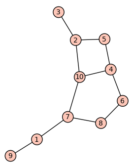
The instructions in SAGE for create this graphs area

sage: X1=Graph([(1, 7), (1, 8), (1, 10), (2, 3), (3, 6),
      (4, 5), (5, 6), (6, 10), (7,9), (7, 10), (8, 9)])
sage: X2=Graph([(1, 7), (1, 9), (2, 3), (2, 5), (2, 10),
      (4, 5), (4, 6), (4, 10), (6,8), (7, 8), (7, 10)])
sage: Isomorphism(X1,X2,10)
False

Now, we will present some graphics of different time tests. The first graphic, Figure 4.5, shows the time expend by the algorithm to test if two random graphs are isomorphic. The times are so small because if we take two random graphs probably will take a different number of edges. Although in the major part of the example the algorithm ends because the graphs have a different time of edges, sometimes the algorithm enters in the loop, and in this case the algorithm is relatively efficient.

To make the graphs more similar, we perform another test. In this example the degree of the first $n-1$ nodes are the same and the last is chosen randomly, this way a third part of the graphs will be isomorphic. In this case, we also have reasonable times and the relation time-nodes can be seen in Figure 4.6 and Figure 4.7

Finally, we will show what happens if we test isomorphic graphs. In this case the time grows, but we can see in Figure 4.8 that the time grows more slowly than $(x/10)^{3}$ . The Figure 4.8 shows the comparison between the algorithm and the functions $(x/10)^{4},(x/10)^{3},(x/10)^{2}\log(x/10),(x/10)^{2}$

Sumario

En este trabajo haremos un estudio teórico de un algoritmo para isomorfismo de grafos de valencia acotado propuesto por Eugene M. Luks(1982) y una implementación en el sistema SAGE de dicho algoritmo para el caso de valencia 3.

Este trabajo tiene 4 partes claramente diferenciadas, a saber:

1.

Preliminares
2.

Algoritmos previos
3.

Algoritmo principal
4.

Pruebas de la implementación

Preliminares

En los preliminares tenemos 3 partes: teoría de grupos, teoría de grafos y teoría de la complejidad.

En la primera presentamos las definiciones básicas de teoría de grupos centrandonos en el grupo de permutaciones, así definiciones importantes que se ven son orbita, transitividad, G-block y G-block system.

En la segunda, las definiciones básicas de teoría de grafos, como por ejemplo que és un isomorfismo entre grafos, también presentamos algunos resultados, como por ejemplo que el conjunto de automorfismos de un grafo forman un grupo.

Finalmente en la tercera y última parte mostraremos conceptos generales sobre complejidad, algoritmos polinomiales y una idea intuitiva de reducibilidad.

Algoritmos previos

En este capítulo presentamos dos tipos de algoritmos, primero veremos algoritmos que se basan en teoría de grupos y luego otros dentro de la teoría de grafos.

Algoritmos básicos en teoría de grupos

Lo más importante y destacable son los dos lemas siguientes:

Lemma 15 (Furst-Hopcroft-Luks).

Dado un conjunto de generadores para un subgrupo $G$ de $S_{n}$ se puede determinar en tiempo polinómico

1.

El orden de $G$ .
2.

Saber si una permutación $\sigma$ pertenece a $G$ .
3.

Los generadores de un subgrupo de $G$ que sabemos que el índice en $G$ tiene una cota polinomial y, tenemos un test de pertenencia que se puede ejecutar en tiempo polinomial.

Lemma 16.

Dado un conjunto de generadores para un subgrupo $G$ de $S_{n}$ y una $G-$ orbita $B$ , se puede determinar en tiempo polinomial, un $G-$ block system minimal en $B$ .

Con el primer lema obtenemos el Algoritmo 7 y, con el segundo obtenemos el Algoritmo 8, que serán importantes en el algoritmo principal.

Algorithm 7 Filter

Data:

\alpha\in G

Result: Add

\alpha

to his

C_{i}

1 begin

2 for $i\in[0,n-2]$ do

3 if $\mathop{\mathstrut{\exists}}\nolimits\gamma\in C_{i}\mbox{ : }\gamma^{-1}\alpha\in G_{i+1}$ then

\alpha\leftarrow\gamma^{-1}\alpha

5 else

6 add

\alpha

C_{i}

7 return

8 return

Algorithm 8 Smallest

G-

block which contains

\{1,\omega\}

Data:

\omega\neq 1

G=\langle g_{1},\ldots,g_{m}\rangle

Result: The smallest

G-

block which contains

\{1,\omega\}

1 begin

C\leftarrow\varnothing

3 Set

f(\alpha=\alpha)\;\mathop{\mathstrut{\forall}}\nolimits\alpha\in A

4 Add

\omega

C

5 Set

f(\omega)=1

6 while $C$ is nonempty do

7 Delete

\beta

from

C

\alpha\leftarrow f(\beta)

j\leftarrow 0

10 while $j<m$ do

j++

\gamma\leftarrow\alpha g_{j}

\delta=\beta g_{j}

14 if $f(\gamma)\neq f(\delta)$ then

15 Ensure

f(\delta)<f(\gamma)

by interchanging

\gamma

and

\delta

if necessary.

16 for $\epsilon\;:\;f(\epsilon)=f(\gamma)$ do

17 Set

f(\epsilon)=f(\delta)

18 Add

f(\gamma)

C

19 return C

Algoritmos básicos en teoría de grafos

En esta parte se muestra un ejemplo ilustrando que no siempre es un problema complicado el saber si dos grafos son isomorfos. Para Mostramos un algoritmo que es $O(n)$ para el isomorfismo de arboles filogenéticos, este lo presentamos en Algoritmo 9

Algorithm 9 PhylogeneticTreeIsomorphism

Data:

T_{1}=(T_{1},\rho_{1},\{u_{1},\ldots,u_{2}\})andT_{2}=(T_{2},\rho_{2},\{u_{1},\ldots,u_{2}\})

Result: Test if

T_{1}

and

T_{2}

are isomorphic

1 begin

2 Set

\varphi(\rho_{1}(u_{i}))=\rho_{2}(u_{i})\;\mathop{\mathstrut{\forall}}\nolimits i

3 Nodes

\leftarrow

PostOrderIterator( $T_{1}$ )

w\leftarrow Nodes.next()

5 while Nodes.hasNext() do

6 if $w$ is not a leaf then

7 if $\varphi(w)==$ none then

v

child of

w

9 Set

\varphi(w)=parent(\varphi(v))

10 for $v$ child of $w$ do

11 if $\varphi(w)\neq$ parent( $\varphi(v)$ ) then

12 return False

13 return $\varphi$

Algoritmo principal

En este capítulo veremos el algoritmo principal. La idea general se muestra en el Algoritmo 10.

Algorithm 10 Isomorphism of graphs of bounded valence

Data:

X_{1},X_{2}

connected graphs of bounded valence

Result: Test if

X_{1}

and

X_{2}

are isomorphic

1 begin

e_{1}\in\mathcal{E}(X_{1})

3 for $e_{2}\in\mathcal{E}(X_{2})$ do

X\leftarrow

BuildX( $X_{1},X_{2},e_{1},e_{2}$ )

G\leftarrow

Aut (

X,e

)

6 for $\sigma\in G$ do

7 if $\sigma(v_{1})==v_{2}$ then

8 return True

9 return False

La estructura de este capítulo esta dividida como sigue:

•

Valencia 3.
•

Estudio de la complejidad para el caso de valencia 3.
•

Mejoras para la implementación.
•

Generalización al caso general

Valencia 3

En esta parte mostramos como funciona el algoritmo cuando los grafos tienen valencia 3. Para eso, calculamos el grupo de automorfismos de un grafo, con este fin computamos una sucesión de grafos y creamos una serie de homomorfismos entre los grupos de automorfismos de esa sucesión de grafos. Aqui usaremos el Algoritmo 11 y obtendremos la sucesión de automorfismos que queríamos.

Algorithm 11 The group

Aut_{e}

Data: A sequence of graphs

Y

, whose are the result of BuildX

Result:

Aut_{e}(X)

where

X

is the last graph in the sequence

1 begin

Aut_{e}=(e_{1}\;e_{2})

for $X\in Y$ do

K\leftarrow

Ker (

X

)

S\leftarrow

Image (

Aut_{e},X

)

S2\leftarrow

Pullback (

S,X

)

Aut_{e}=S2\cup K

7 return $Aut_{e}$

Estudio de la complejidad

En esta parte mostramos de manera más detallada que el algoritmo anterior es polinómico y, que $O(n^{10})$ es una cota superior del coste de dicho algoritmo.

Mejora para la implementación

Dedicamos esta parte al estudio de mejoras en vistas de la implementación, estas mejoras serán:

•

Reducir el tamaño de $A_{r}$ .
•

Representar los grupos mediante SGS.
•

Precomputar los bloques.
•

Otras mejoras.

Con estas mejoras conseguiremos que el algoritmo sea $O(n^{4})$ , en el peor de los casos.

Caso general

Finalmente veremos que para el caso general lo único que necesitamos es comprobar que el núcleo de los homomorfismos sigue siendo un 2-grupo y, por lo tanto podremos aplicar todo lo demás, adaptándolo para cada valencia.

Pruebas de la implementación

Finalmente presentamos algunos tests realizados con la implementación en el sistema SAGE, con estos mostramos que la cota superior de $O(n^{4})$ no se alcanza y, que en el caso medio el algoritmo tiene un coste, informalmente, entre $O(n^{3})$ y $O(n^{2}\log n)$ .

El apéndice mostramos la documentación de la implementación, aunque se recomienda al lector visitar la pagina http:// www.alumnos.unican.es/aam35/sage-epydoc/index.html donde hay una detallada documentación en HTML mucho más fácil y ágil de usar.

Bibliography

[1] Alfred V. Aho and John E. Hopcroft. The Design and Analysis of Computer Algorithms. Addison-Wesley Longman Publishing Co., Inc., Boston, MA, USA, 1st edition, 1974.
[2] M. D. Atkinson. An algorithm for finding the blocks of a permutation group. Mathematics of Computation, 29(131):pp. 911–913, 1975.
[3] M. D. Atkinson, R. A. Hassan, and M. P. Thorne. Group theory on a micro-computer. Computation Group Theory, pages 275–280, 1984.
[4] László Babai and Eugene M. Luks. Canonical labeling of graphs. In STOC, pages 171–183, 1983.
[5] K S Booth and C J Colbourn. Problems polynomially equivalent to graph isomorphism. Technical report, 1977.
[6] Thomas H. Cormen, Clifford Stein, Ronald L. Rivest, and Charles E. Leiserson. Introduction to Algorithms. McGraw-Hill Higher Education, 2nd edition, 2001.
[7] Zvi Galil, Christoph M. Hoffmann, Eugene M. Luks, Claus P. Schnorr, and Andreas Weber. An $o(n^{3}\log n)$ deterministic and an $o(n^{3})$ las vegas isomorphism test for trivalent graphs. Journal of hte Association for Computing Machinery, 34(3):513–531, 1987.
[8] M. Hall. The theory of groups. AMS Chelsea Publishing Series. AMS Chelsea Pub., 1976.
[9] Mark Jerrum. A compact representation for permutation groups. Journal of Algorithms, 7(1):60–78, 1986.
[10] Susan Landau and Gary L. Miller. Solvability by radicals is in polynomial time. Journal of Computer and System Sciences, 30(2):179–208, April 1985. invited publication.
[11] Eugene M. Luks. Isomorphism of graphs of bounded valence can be tested in polynomial time. Journal of Computer and System Sciences, 25(1):42–65, 1982.
[12] Volker Nannen. The Paradox of Overfitting. Master’s thesis, Rijksuniversiteit Groningen, the Netherlands, 2003.
[13] J.S. Rose. A course on group theory. Cambridge University Press, 1978.
[14] Ákos Seress. Permutation Group Algorithms. Cambridge tracts in mathematics 152. Cambridge University Press, 2003.
[15] Charles C. Sims. Graphs and finite permutation groups. Mathematische Zeitschrift, 95:76–86, 1967. 10.1007/BF01117534.

Index

ancestor Definition 10
$Aut(G)$ Proposition 2
binary evolutionary network Definition 13
block of imprimitivity §1.1
children Definition 10
connected graph Definition 5
cycle Definition 4
degree Definition 6
edge §1.2
evolutionary network Definition 12
faithful §1.1
$G$ -block Definition 2
$G-$ block system §1.1
$G-$ orbit Definition 1
graph §1.2
isomorphism Definition 8
minimal, $G-$ block system §1.1
P Definition 14
parent Definition 10
path Definition 4
permutation group §1.1
phylogenetic tree Definition 11
Polynomial reduction Definition 15
primitive §1.1
Pruned tree Definition 19
Smooth generating sequence Definition 17
stabilize §1.1
Structure tree Definition 18
symmetric group §1.1
tree Definition 10
tree node §1.2
twins Definition 16
valence Definition 7
vertex §1.2

13*