Ternary graph isomorphism in polynomial time, after Luks
Abstract
The graph isomorphism problem has a long history in mathematics and computer science, with applications in computational chemistry and biology, and it is believed to be neither solvable in polynomial time nor NP-complete. E. Luks proposed in 1982 the best algorithm so far for the solution of this problem, which moreover runs in polynomial time if an upper bound for the degrees of the nodes in the graphs is taken as a constant. Unfortunately, Luks’ algorithm is purely theoretical, very difficult to use in practice, and, in particular, we have not been able to find any implementation of it in the literature. The main goal of this paper is to present an efficient implementation of this algorithm for ternary graphs in the SAGE system, as well as an adaptation to fully resolved rooted phylogenetic networks on a given set of taxa.
1 Introduction
The graph isomorphism problem —the problem of deciding whether two finite graphs are isomorphic or not— has a long history in mathematics and computer science. It is one of the most important decision problems for which the computational complexity is not known yet [11, 16], and it is believed to be neither in P nor NP-complete. Its uncertain status has led to the definition and study of the class GI of the decision problems that are polynomial-time Turing reducible to it [13].
The best current theoretical algorithm for the solution of the graph isomorphism problem is due to Eugene Luks [18, 19]. His algorithm runs in time , where is the number of nodes in the graphs, and it relies on the classification of finite simple groups [6]. Without using this major result, whose proof consists of tens of thousands of pages in several hundred journal articles and for which a unified, simplified and revised version is still in progress, Babai and Luks [3] gave an algorithm that runs in time.
The graph isomorphism problem has many practical applications outside mathematics. Our interest in it stems from its applications in computational biology and bioinformatics. Graphs are ubiquitous in biology as models of different complex systems: molecular structures, phylogenetic trees and networks, metabolical pathways, protein-protein interaction (PPI) networks, gene expression networks, etc. [2, 14, 15, 20]. In all these fields, the comparison of graphs is an important computational problem. For instance, a protein’s function is closely related to its three-dimensional shape, which at an intermediate level of detail is modeled by a contact graph, and thus the comparison of such contact graphs is a key tool in the prediction of proteins’ function [12, 23]; the comparison of phylogenies is acknowledged to be one of the main problems in phylogenetics [7, 15, 22]; and the comparison of metabolic pathways and PPI networks is currently one of the hot tools in the study of evolution [8, 17]. The most basic graph comparison problem in all these contexts is, of course, the detection of equalities. Without being able to decide efficiently whether two such graphs are isomorphic or not, we cannot expect to define metrics, matchings or alignments that can be computed efficiently.
So, it is important to design efficient algorithms to test if two graphs are isomorphic, at least for some special classes of graphs with practical applications. The aforementioned algorithm by Luks [19] is fixed-parameter tractable, in the sense that it runs in polynomial time if we consider an upper bound for the degrees of the graphs under comparison as a constant. Such an algorithm, even for ternary graphs (graphs with all their nodes of degree at most 3), has relevant applications in computational biology: for instance, in phylogenetics, in the comparison of arbitrary fully resolved rooted phylogenetic networks, and in the comparison of split networks [15]; in both types of networks, all nodes have total degrees at most 3. For these networks, no specific polynomial-time isomorphism test has been devised yet, and the authors working with them simply quote Luks’ result when they need to state that their isomorphism can be decided in polynomial time; see, for instance, [15, p. 168] or [4, §V].
The problem with Luks’ algorithm is that it is purely theoretical, very difficult to use in practice, and, in particular, we have not been able to find any implementation of it in the literature. The main goal of this paper is, then, to present an efficient implementation of this algorithm in the SAGE system. We also present an implementation of an adaptation of this algorithm that solves the isomorphism problem for fully resolved rooted phylogenetic networks. This paper is based on the first author’s Master Thesis [1], where we refer the reader for more details.
2 Luks’ algorithm for ternary graphs
In this section we explain Luks’ algorithm for ternary graphs, that is, for connected graphs with all their nodes of degree at most . We shall omit all proofs, which can be found in the original paper by Luks [19] or, with more detail, in the first author’s Master Thesis [1].
We begin by reducing the graph isomorphism problem to a problem about isomorphisms of groups. Given two ternary graphs and , and two edges and , consider the ternary graph obtained by splitting and by means of new nodes and , respectively, and then connecting these new nodes and by means of a new edge . Then, and are isomorphic if, and only if, given any , there exist some and some automorphism of such that , and in particular such that . And then, if any such automorphism of does exist, then any set of generators of , the group of automorphisms of that fixes , will contain some. This provides the following algorithm.
So, we are reduced to compute a set of generators of , for a ternary graph and any . This group is determined through a natural sequence of successive “approximations” , where each is the subgraph consisting of all nodes and all edges of which appear in paths of length containing . More formally, if , let
and, for every ,
There exist natural homomorphisms
defined by the restriction of the automorphisms. These homomorphisms allow us to construct recursively a generating set for from one for by solving, for every , the following two problems:
- (I)
Compute a set of generators of .
- (II)
Compute a set of generators of .
Indeed, if is any set of pre-images of in , then generates .
So, if we know how to solve Problems I and II, the algorithm to compute a set of generators of is the following. In it, and in the sequel, given two elements of a set , we denote by the transposition .
Set now and , and consider the mapping
defined by ; we call the neighbor set of . The following result solves Problem I.
Proposition 1
Moreover, the fact that each is generated by transpositions implies, by induction, the following result, which will be useful later.
Proposition 2
For each , is a -group.
So, our graph isomorphism problem is reduced to solve Problem II. Now, consider the following three subsets of :
We have the following result.
Proposition 3
is the set of those that stabilize the sets , , and .
Now, set and extend the action of on to in the natural way: if , then . Color each element of with one of five colors that distinguish, on the one hand, whether or not it is in , and, on the other hand, whether it is in , or , or neither. Only five colors are needed, since .
By the previous proposition, if and only if preserves these colors in . Therefore, the isomorphism problem for ternary graphs is polynomial-time reducible to the following color automorphism problem (taking , , ).
Problem 1
Given
- •
A set of generators for a -subgroup of the symmetric group of a colored set
- •
A -stable subset
- •
A permutation
find , where, for every
Now, the following three lemmas are the basis of Algorithm 3 that solves Problem 1 in polynomial-time, and thus it completes the graph isomorphism test we were looking for.
Lemma 1
Let be a subgroup of , and a -stable subset of such that is not empty. Then, is a subgroup of and it is a left coset of the subgroup .
Lemma 2 (Furst-Hopcroft-Luks [9])
Given a set of generators of a subgroup of a symmetric group, one can compute in polynomial time a set of generators of any subgroup of that is known to have polynomially bounded index in and for which a polynomial-time membership test is available.
Lemma 3 (Luks [19])
Given a set of generators of a subgroup of a symmetric group and a -orbit , one can determine in polynomial time a minimal -block system in .
Theorem 2.1
Algorithm 1 solves the ternary graph isomorphism in time , with the size of the input graphs.
Proof
The cost of computing BuildX applied to a pair of graphs of size and a pair of edges is in time. For every , a set of generators of can be computed as explained in Lemma 1 in time, a set of generators of can be computed, by reducing this computation to Problem 1 and then using Algorithm 3, in time, and a set of preimages in of the latter can be computed in time. Since there are at most indices , we conclude that the cost of computing a set of generators of by means of Algorithm 2 is in . Since Algorithm 1 calls Algorithm 2 times, the final cost of Algorithm 1 is in .
3 Implementation
3.1 Improvements
In our implementation we have improved the efficiency of Luks’ algorithm by:
- (a)
Reducing the size of the set .
- (b)
Representing the groups by means of smooth generating sequences.
- (c)
Precomputing the blocks.
- (d)
Running initial tests, to avoid trivial cases.
- (e)
Removing, for every , the permutations that do not swap the two “parts” and of .
With these improvements, the cost of the computation decreases to . We explain now in some detail the improvements (a)–(c), which were inspired by [10]. For more details, see [1].

As far as improvement (a) goes, we have been able to remove the triplets from , by replacing each node with a 3-elements neighbor set by a triangle with nodes at “level” and labeled edges: cf. Figure 1. In this way, we can replace the graph by a new graph with some edges labeled. The automorphisms of must preserve labels, and therefore the computation of is the same as that of , except for the following facts: needs only to include the subsets of of size 1 or 2; we split into
and we modify the set of colors on to distinguish, on the one hand, whether or not an element is in , or , or neither, and, on the other hand, whether it is in , or , or neither.
As to (b), we represent 2-groups in a way that makes easier several key computations.
Definition 1
Let be a 2-group generated by . The sequence is a smooth generating sequence (SGS, for short) for if , for .
SGS are preserved by homomorphisms and liftings, and if we know a SGS for a 2-group , then it is easy construct an SGS for a subgroup of index 2 [10].
Lemma 4
Let be a 2-group, a SGS for it, and a subgroup of index 2. Let and set, for ,
Then is a SGS for , and this sequence is computed in times the required time of a membership test for .
Let us consider finally improvement (c). As we have seen in the proof of Theorem 2.1, the most expensive part of Luks’ algorithm is the recursive calls performed by Algorithm 3. The task carried out by this algorithm can be reorganized so as to limit the number of different blocks visited. These blocks form a tree that is precomputed and guides the recursion.
Definition 2
Let be a 2-group acting on a stable subset of a colored set . We call a binary tree a structure tree for with respect to , , if the set of leaves of is , and the action of any on can be lifted to an automorphism of .
Let be a fixed color of (in our application, it will be the color of the elements of that do not belong to ). A node of will be called active if . An active node is facile if is intransitive on and the latter has exactly one active child. Let denote the closest non facile descendant of in .
We can precompute the entire structure tree for a given pair using Algorithm 4 below. With this algorithm, we can construct every structure tree in time, and we can compute the mapping and the set of active nodes in time. Using structure trees to guide the recursion, the cost of computing decreases to .
3.2 Implementation details
We have implemented Luks’ algorithm using the language Python and some specific SAGE libraries for handling graphs and groups of permutations.
Besides the obvious classes and functions necessary to implement the algorithm, we use a new class, called Node, for the structure tree. This class has four attributes:
- •
Node, the content of the node.
- •
Left, the left child.
- •
Right, the right child.
- •
Parent, the parent.
When we build a new Node without some attributes, they will be empty arrays. This class has the necessary functions to modify its attributes, as well as the following functions:
- •
IsLeaf(), to know whether the node is a leaf.
- •
Istransitive(), to know whether is transitive on the node.
- •
Isactive(Q), to know whether the node is active w.r.t. .
- •
Isfacile(Q), to know whether the node is facile w.r.t. .
- •
Delta(Q), to know the nearest non facile descendant of the node.
To test whether two graphs are isomorphic or not, we can use two different functions, Isomorphism and Isomorphism2. Both functions answer the question whether the input graphs are isomorphic, but moreover the first function returns the whole group of automorphisms that fix the distinguished edge of the graph , while the second one only returns the subgroup of those automorphisms of that swap the parts and .
Finally, we have adapted Luks’ algorithm to test the isomorphism of fully resolved rooted phylogenetic networks on a given set of taxa. A rooted phylogenetic network, on a set of taxa is a rooted, directed, acyclic graph with its leaves bijectively labeled in . These graphs are used as explicit models of evolutionary histories that, besides mutations, include reticulate evolutionary events like genetic recombinations, lateral gene transfers or hybridizations. An evolutionary network is fully resolved , or binary, when, for every node in it, the ordered pair is either (the root), (the leaves), (the tree nodes) or (the reticulate nodes). Two evolutionary networks on are isomorphic when they are isomorphic as directed graphs and the isomorphism preserves the leaves’ labels. For more on phylogenetic networks, see [15].
The main difference between the case of rooted phylogenetic networks and the general case is that, in the former, the isomorphisms map the root to the root, and therefore the graph can be simply obtained by connecting the roots by an edge . In particular, Algorithm 1 needs not to call times Algorithm 2, but only once, and the resulting cost is then in .
To test the isomorphism of fully resolved rooted phylogenetic networks we have defined the function IsomorphismPhilo, which has the following parameters:
- •
X1, the first phylogenetic network.
- •
X2, the second phylogenetic network.
- •
n, the number of nodes of X1.
- •
dic1, the dictionary with the labels of the nodes of the first graph.
- •
dic2, the dictionary with the labels of the nodes of the second graph.
- •
r1, the root of the first graph.
- •
r2, the root of the second graph.
IsomorphismPhilo accepts networks with inner taxa (with internal labeled nodes) as well as multilabeled networks (where different nodes can have the same label), although these features are not used (yet) in the phylogenetic networks literature. For the moment, the algorithm only accepts phylogenetic networks created with SAGE’s function Graph, but in the near future we plan to adapt it so that it accepts networks described in the format eNewick [5].
We have performed several tests on our implementation, which we report in the next subsection. In the first and the third tests, we have used SAGE functions to generate random graphs and we have then made these graphs connected and trivalent, by randomly adding or removing edges when it was necessary. In the second test, we have used the function graphs.DegreeSequence that, given a sequence of degrees, returns a graph whose nodes have this sequence of degrees, if some exists. This has allowed us to know the probability that the graphs under comparison were isomorphic.
To perform the tests on phylogenetic networks we defined some functions to create random fully resolved rooted phylogenetic networks:
- •
createDic(nodes,n), which, given a set of nodes, returns the following dictionary:
- •
createDic2(nodes,n), as above, but the selected nodes are labeled “a” or “b” equiprobably.
- •
leaves(X1), returns the set of nodes of the network X1.
Then, we have developed an algorithm RandomTree(n) that returns a fully resolved rooted phylogenetic network with nodes. By default, each internal node has a probability of of being hybrid, but it can be changed by simply changing the probability parameter from to the desired probability.
The documentation of the whole module can be found in http://www.alumnos.unican.es/aam35/sage-epydoc/index.html and the code in http://www.alumnos.unican.es/aam35/IsoTriGraph.py.
3.3 Tests
The first two examples show that the code works correctly, and then the tests prove that it runs in a reasonable time, comparable to the speed of the own SAGE algorithm to test isomorphisms of graphs.
Example 1
Consider the graphs and depicted in Fig. 2. These graphs are created in SAGE with:
 sage: X3=Graph([(1, 7), (1, 10), (2, 3), (2, 4), (3, 4),(4, 9),
       (5,6),(6, 8), (7, 8), (7, 9),(8, 9)])
 sage: X4=Graph([(2, 3), (2, 10), (1, 7), (1, 4), (7, 4),(4, 9),
       (5, 6),(6, 8), (3, 8), (3, 9),(8, 9)])


We test whether they are isomorphic:
sage: Isomorphism2(X3,X4,10,Iso=True)
1 --> 2
2 --> 1
3 --> 7
4 --> 4
5 --> 5
6 --> 6
7 --> 3
8 --> 8
9 --> 9
10 --> 10
True
And, indeed, it is obvious that this is an isomorphism between and .
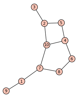
Example 2
Consider now the graphs and depicted in Fig. 3.
sage: X1=Graph([(1, 7), (1, 8), (1, 10), (2, 3), (3, 6),
      (4, 5), (5, 6), (6, 10), (7,9), (7, 10), (8, 9)])
sage: X2=Graph([(1, 7), (1, 9), (2, 3), (2, 5), (2, 10),
      (4, 5), (4, 6), (4, 10), (6,8), (7, 8), (7, 10)])
sage: Isomorphism(X1,X2,10)
False
And, indeed, they are clearly non isomorphic.

Test 3.1
Fig. 4 shows the time needed by Isomorphism2 to test whether two random graphs are isomorphic, as a function of the numbers of nodes in the graphs. The times are so small because two random graphs with the same number of nodes have probably different numbers of edges, a property that our program checks before proceeding with Luks’ algorithm. Although in most cases the algorithm detected non-isomorphism by trivial reasons, the algorithm is also relatively efficient in non trivial cases.

Test 3.2
In this test we fix the degrees of nodes in the graphs, and the degree of the last node is chosen at random. In this way we guarantee that the probability of two graphs being isomorphic is . In this case, our algorithm also runs in reasonable time: see Figs. 5 and 6.


Test 3.3
Fig. 7 shows the times (red dots) needed by the algorithm to detect the isomorphism between pairs of isomorphic graphs with nodes, and it compares this time with the functions , , , and .

Our last test deals with rooted phylogenetic networks.
Test 3.4
Fig. 8 displays the relation running time-number of nodes for our algorithm when applied to random fully resolved rooted phylogenetic networks on the same sets of taxa, and Fig. 9 shows this relation for phylogenetic networks that are isomorphic as undirected graphs but need not be isomorphic as phylogenetic networks.


4 Conclusions
In this paper we have presented our implementation in SAGE of Luks’ polynomial-time algorithm for testing the isomorphism of ternary graphs. This algorithm has interesting applications in phylogenetics, as it allows, for instance, to detect whether two fully resolved rooted phylogenetic networks are isomorphic. Therefore, we have adapted and implemented Luks’ algorithm for this type of graphs. Our adaptation has been, except for one point, a direct translation of Luks’ algorithm. Fully resolved rooted phylogenetic networks have specific characteristics that could be used to improve the algorithm to make it still more efficient in this specific application. It is in our research agenda to develop such an adaptation, and we hope to present it elsewhere.
Acknowledgements. This research has been partially supported by the Spanish government and the UE FEDER program, through project MTM2009-07165. We thank Prof. T. Recio for encouraging us to write this report, and for his comments on a first version of it.
References
- [1] A. Alcala. “ Trivalent Graph Isomorphism in Polynomial Time.”, Master’s thesis, University of Cantabria, Spain, 2012. www.alumnos.unican.es/aam35/MastherThesis.pdf
- [2] T. Aittokallio, B. Schwikowski. “Graph-based methods for analysing networks in cell biology.” Briefings in Bioinformatics 7 (2006), 243–255.
- [3] L. Babai, E. M. Luks. “Canonical labeling of graphs.” 15th STOC (ACM, 1983), 171–183.
- [4] G. Cardona, M. Llabrés, F. Rosselló, G. Valiente. “On Nakhleh’s metric for reduced phylogenetic networks”. IEEE/ACM Transactions on Computational Biology and Bioinformatics 6 (2009), 629–638
- [5] G. Cardona, F. Rosselló, G. Valiente. “Extended Newick: it is time for a standard representation of phylogenetic networks”. BMC Bioinformatics 9:532 (2008).
- [6] D. Gorenstein, R. Lyons, R. Solomon. The classification of the finite simple groups. Mathematical Surveys and Monographs 40 (AMS, 1994).
- [7] J. Felsenstein. Inferring Phylogenies. Sinauer Associates Inc. (2004).
- [8] C. Forst, K. Schulten. “Phylogenetic analysis of metabolic pathways.” J. Mol. Evol. 52 (2001), 471–489.
- [9] M. L. Furst, J. E. Hopcroft, E. M. Luks. “Polynomial-time algorithms for permutation groups.” Proceedings 21st FOCS (IEEE Computer Society, 1980), 36–41.
- [10] Z. Galil, C. M. Hoffmann, E. M. Luks, C.-P. Schnorr, A. Weber. “An O(n(n)) deterministic and an O(n3) Las Vegas isomorphism test for trivalent graphs.” J. ACM 34 (1987), 513–53.
- [11] M. Goldberg. “The graph isomorphism problem.” In: Handbook of Graph Theory (J. L. Gross and J. Yellen eds.) (CRC Press, 2003) 68–78.
- [12] C. Guerra, S. Istrail (eds). Mathematical Methods for Protein Structure Analysis and Design. Lecture Notes in Computer Science 2666 (Springer, 2003)
- [13] C. M. Hoffmann, Group-theoretic algorithms and graph isomorphism. Lecture Notes in Computer Science 136, Springer-Verlag (1982).
- [14] W. Huber, V. J. Carey, L. Long, S. Falcon, R. Gentleman. “Graphs in molecular biology.” BMC Bioinformatics 8(Suppl 6):S8 (2007).
- [15] D. H. Huson, R. Rupp, C. Scornavacca. Phylogenetic Networks: Concepts, Algorithms and Applications. Cambridge University Press (2011).
- [16] J. Köbler, U. Schöning, J. Torán. The graph isomorphism problem: Its structural complexity. Birkhäuser (1993).
- [17] M. Koyorturk, Y. Kim, U. Topkara, S. Subramaniam, W. Szpankowski, A. Grama. “Pairwise alignment of protein interaction networks.” J. Comp. Biol. 13 (2006), 182–199.
- [18] E. M. Luks. “Isomorphism of graphs of bounded valence can be tested in polynomial time.” Proceedings 21th FOCS (IEEE Computer Society, 1980), 42–49.
- [19] E. M. Luks. “Isomorphism of graphs of bounded valence can be tested in polynomial time.” Journal of Computer and System Sciences 25 (1982), 42–65.
- [20] O. Mason, M. Verwoerd. “Graph theory and networks in biology.” IET In Systems Biology, 1 (2007), 89–119
- [21] D. A. Spielman. “Faster isomorphism testing of strongly regular graphs.” Proceedings 28th STOC (ACM, 1996), 576–584.
- [22] M. A. Steel, D. Penny, “Distributions of tree comparison metrics—some new results.” Systematic Biology 42 (1993), 126–141.
- [23] W. Taylor, A. Aszódi. Protein Geometry: Classification, Topology and Symmetry. Inst. Physics Publ. (2005).