Exponential synchronization rate of Kuramoto oscillators in the presence of a pacemaker

Yongqiang Wang Member, IEEE Francis J. Doyle III Fellow, IEEE ^†^†thanks: The work was supported in part by U.S. ARO (W911NF-07-1-0279), NIH (GM078993), and ICB (W911NF-09-0001) from the U.S. ARO. The content of the information does not necessarily reflect the position or the policy of the Government, and no official endorsement should be inferred.^†^†thanks: Yongqiang Wang, Francis J. Doyle III are with the Institute for Collaborative Biotechnologies, University of California, Santa Barbara, California 93106-5080 USA. E-mail: wyqthu@gmail.com, frank.doyle@icb.ucsb.edu.

Abstract

The exponential synchronization rate is addressed for Kuramoto oscillators in the presence of a pacemaker. When natural frequencies are identical, we prove that synchronization can be ensured even when the phases are not constrained in an open half-circle, which improves the existing results in the literature. We derive a lower bound on the exponential synchronization rate, which is proven to be an increasing function of pacemaker strength, but may be an increasing or decreasing function of local coupling strength. A similar conclusion is obtained for phase locking when the natural frequencies are non-identical. An approach to trapping phase differences in an arbitrary interval is also given, which ensures synchronization in the sense that synchronization error can be reduced to an arbitrary level.

Index Terms:

Exponential synchronization rate, Kuramoto model, pacemaker, oscillator networks

I Introduction

The Kuramoto model was first proposed in 1975 to model the synchronization of chemical oscillators sinusoidally coupled in an all-to-all architecture [1]. Although it is elegantly simple, the Kuramoto model is sufficiently flexible to be adapted to many different contexts, hence it is widely used and is regarded as one the most representative models of coupled phase oscillators [2]. Recently, the Kuramoto model has received increased attention. For example, the authors in [3, 4, 5] discussed synchronization conditions for the Kuramoto model. The work in [6] gave a synchronization condition for delayed Kuramoto oscillators. Results are also obtained for Kuramoto oscillators with coupling topologies different from the original all-to-all structure. For example, the authors in [7] and [8] considered the phase locking of Kuramoto oscillators coupled in a ring and a chain, respectively. Using graph theory, the authors in [9, 10, 11] discussed the synchronization of Kuramoto oscillators with arbitrary coupling topologies. The authors in [12] proved that exponential synchronization can be achieved for Kuramoto oscillators when phases lie in an open half-circle.

Studying the influence of the pacemaker (also called the leader, or the pinner [13]) on Kuramoto oscillators is not only of theoretical interest, but also of practical importance [14, 15]. For example, in circadian systems, thousands of clock cells in the brain are entrained to the light-dark cycle [16]. In the clock synchronization of wireless networks, time references in individual nodes are synchronized by means of intercellular interplay and external coordination from a time base such as GPS [17]. Hence, Kuramoto oscillators with a pacemaker are attracting increased attention. The authors in [14] and [18] studied the bifurcation diagram and the steady macroscopic rotation of Kuramoto oscillators forced by a pacemaker that acts on every node. Based on numerical methods, the authors in [19] showed that the network depth (defined as the mean distance of nodes from the pacemaker, a term closely related to pinning-controllability in pinning control [20]) affects the entrainment of randomly coupled Kuramoto oscillators to a pacemaker. Using numerical methods, the authors in [21] discovered that there may be situations in which the population field potential is entrained to the pacemaker while individual oscillators are phase desynchronized. But compared with the rich results on pacemaker-free Kuramoto oscillators, analytical results are relative sparse for Kuromoto oscillators forced by a pacemaker. And to our knowledge, there are no existing results on the synchronization rate of arbitrarily coupled Kuramoto oscillators in the presence of a pacemaker.

The synchronization rate is crucial in many synchronized processes. For example, in the main olfactory system, stimulus-specific ensembles of neurons synchronize their firing to facilitate odor discrimination, and the synchronization time determines the speed of olfactory discrimination [22]. In the clock synchronization of wireless sensor networks, the synchronization rate is a determinant of energy consumption, which is vital for cheap sensors [23, 24].

We consider the exponential synchronization rate of Kuramoto oscillators with an arbitrary topology in the presence of a pacemaker. In the identical natural frequency case, we prove that synchronization (oscillations with identical phases) can be ensured, even when phases are not constrained in an open half-circle. In the non-identical natural frequency case where perfect synchronization has been shown cannot be achieved [2],[25], we prove that phase locking (oscillations with identical oscillating frequencies) can be ensured and synchronization can be achieved in the sense that phase differences can be reduced to an arbitrary level. In both cases, the influences of the pacemaker and local coupling strength on the synchronization rate are analyzed.

II Problem formulation and Model transformation

Consider a network of $N$ oscillators, which will henceforth be referred to as ’nodes’. All $N$ nodes (or a subset) receive alignment information from a pacemaker (also called the leader, or the pinner [13]). Denoting the phases of the pacemaker and node $i$ as $\varphi_{0}$ and $\varphi_{i}$ , respectively, the dynamics of the Kuramoto oscillator network can be written as

\displaystyle\left\{\begin{aligned} \dot{\varphi}_{0}&=w_{0}\\ \dot{\varphi}_{i}&=w_{i}+\hskip-5.69046pt\sum\limits_{j=1,j\neq i}^{N}\hskip-5.69046pta_{i,j}\sin\left(\varphi_{j}-\varphi_{i}\right)+g_{i}\sin\left(\varphi_{0}-\varphi_{i}\right)\end{aligned}\right.

(1)

for $1\leq i\leq N$ , where $w_{0}$ and $w_{i}$ are the natural frequencies of the pacemaker and the $i$ th oscillator, respectively, $a_{i,j}\sin\left(\varphi_{j}-\varphi_{i}\right)$ is the interplay between node $i$ and node $j$ with $a_{i,j}\geq 0$ denoting the strength, $g_{i}\sin(\varphi_{0}-\varphi_{i})$ denotes the force of the pacemaker with $g_{i}\geq 0$ denoting its strength. If $a_{i,j}=0$ (or $g_{i}=0$ ), then oscillator $i$ is not influenced by oscillator $j$ (or the pacemaker).

Assumption 1

We assume symmetric coupling between pairs of oscillators, i.e., $a_{i,j}=a_{j,i}$ .

Next, we study the influences of the pacemaker, $g_{i}$ , and local coupling, $a_{i,j}$ , on the rate of exponential synchronization.

Solving the first equation in (1) gives the dynamics of the pacemaker $\varphi_{0}=w_{0}t+\phi_{0}$ , where the constant $\phi_{0}$ denotes the initial phase. To study if oscillator $i$ is synchronized to the pacemaker, it is convenient to study the phase deviation of oscillator $i$ from the pacemaker. So we introduce the following change of variables:

\displaystyle\varphi_{i}=\varphi_{0}+\xi_{i}=w_{0}t+\phi_{0}+\xi_{i}

(2)

$\xi_{i}\in[-2\pi,\,2\pi]$ denotes the phase deviation of the $i$ th oscillator from the pacemaker. Due to the $2\pi$ -periodicity of the sine-function, we can restrict our attention to $\xi_{i}\in[-\pi,\,\pi]$ . Substituting (2) into (1) yields the dynamics of $\xi_{i}$ :

\displaystyle\begin{aligned} \dot{\xi}_{i}=w_{i}-w_{0}+\sum\limits_{j=1,j\neq i}^{N}a_{i,j}\sin\left(\xi_{j}-\xi_{i}\right)-g_{i}\sin(\xi_{i})\end{aligned}

(3)

Since $\xi_{i}$ is the relative phase of the $i$ th oscillator with respect to the phase of the pacemaker, it will be referred to as relative phase in the remainder of the paper.

By studying the properties of (3), we can obtain:

•

Condition for synchronization: If all $\xi_{i}$ converge to $0$ , then we have $\varphi_{1}=\varphi_{2}=\ldots=\varphi_{N}=\varphi_{0}$ when $t\rightarrow\infty$ , meaning that all nodes are synchronized to the pacemaker.
•

Exponential synchronization rate: The rate of synchronization is determined by the rate at which $\xi_{i}$ decays to $0$ , namely, it can be measured by the maximal $\alpha$ satisfying

$\|\xi(t)\|\leq Ce^{-\alpha t}\|\xi(0)\|,\quad\xi=[\xi_{1},\,\xi_{2},\,\ldots,\,\xi_{N}]^{T}$ (4)

for some constant $C$ , where $\|\bullet\|$ is the Euclidean norm. $\alpha$ measures the exponential synchronization rate of (3): a larger $\alpha$ leads to a faster synchronization rate.

Remark 1

When $w_{i}$ and $w_{0}$ are non-identical, synchronization ( $\xi_{i}=0$ ) cannot be achieved in general. But we will prove in Sec. IV-C that the synchronization error can be made arbitrarily small by tuning the strength of the pacemaker $g_{i}$ .

Assigning arbitrary orientation to each interaction, we can get the $N\times M$ incidence matrix $B$ ( $M$ is the number of interaction edges, i.e., non-zero $a_{i,j}\,(1\leq i\leq N,\,j<i)$ ) of the interaction graph [26]: $B_{i,j}=1$ if edge $j$ enters node $i$ , $B_{i,j}=-1$ if edge $j$ leaves node $i$ , and $B_{i,j}=0$ otherwise. Then using graph theory, (3) can be recast in a matrix form:

\dot{\xi}=\Omega-G\sin\xi-BW\sin\left(B^{T}\xi\right)

(5)

where $\Omega=[w_{1}-w_{0},\,w_{2}-w_{0},\,\ldots,\,w_{N}-w_{0}]^{T}$ , $G=\textrm{diag}(g_{1},\>g_{2},\>\ldots,\>g_{N})$ , and $W=\textrm{diag}(\nu_{1},\>\nu_{2},\>\ldots,\>\nu_{M})$ . Here $\nu_{i}\,(1\leq i\leq M)$ are a permutation of non-zero $a_{i,j}\,(1\leq i\leq N,j<i)$ and $\textrm{diag}(\bullet)$ denotes a diagonal matrix.

III The identical natural frequency case

When $w_{1}=w_{2}=\ldots=w_{N}=w_{0}$ , (5) reduces to:

\dot{\xi}=-G\sin\xi-BW\sin\left(B^{T}\xi\right)

(6)

To study the exponential synchronization rate, we first give a synchronization condition:

Theorem 1

For the network in (6), denote $\varepsilon\triangleq\max\limits_{1\leq i\leq N}|\xi_{i}|$ and ${\rm sinc}(x)\triangleq\sin(x)/x$ , then

1.

when $\varepsilon<\frac{\pi}{2}$ , the network synchronizes if at least one $g_{i}$ is positive and the coupling $a_{i,j}$ is connected, i.e., there is a multi-hop link from each node to every other node;

when $\frac{\pi}{2}\leq\varepsilon<\pi$ , the network synchronizes if the following inequality is satisfied:

		$\displaystyle g_{\min}>$		(7)
		$\displaystyle\max\hskip-2.84544pt\left\{\hskip-2.84544pt\frac{{\rm sinc}(2\varepsilon_{0})\lambda_{\max}(BWB^{T})}{-{\rm sinc}(\varepsilon)},\>\max\limits_{i}\big\{\hskip-5.69046pt\sum\limits_{j=1,j\neq i}^{N}\frac{a_{i,j}}{\sin(\varepsilon)}\big\}\right\}$		(7)

where $\lambda_{\max}(\bullet)$ denotes the maximal eigenvalue, $g_{\min}$ and $\varepsilon_{0}\in(\frac{\pi}{2},\,\pi)$ are determined by

\displaystyle\hskip-5.69046ptg_{\min}=\min\{g_{1},\ldots,g_{N}\},\,2\varepsilon_{0}\cos\left(2\varepsilon_{0}\right)=\sin(2\varepsilon_{0})

(8)

Proof:

We first prove that when $\xi\in[-\varepsilon,\,\varepsilon]\times\ldots\times[-\varepsilon,\,\varepsilon]=[-\varepsilon,\,\varepsilon]^{N}$ where $\times$ denotes Cartesian product, they will remain in the interval under conditions in Theorem 1, i.e, the $n$ -tuple set $[-\varepsilon,\,\varepsilon]^{N}$ is positively invariant for (6).

To prove the positive invariance of $[-\varepsilon,\,\varepsilon]^{N}$ , we only need to check the direction of vector field on the boundaries. When $\varepsilon<\frac{\pi}{2}$ , if $\xi_{i}=\varepsilon$ , we have $-\pi<-2\varepsilon\leq\xi_{j}-\xi_{i}\leq 0$ for $1\leq j\leq N$ . So in (3), $\sin(\xi_{j}-\xi_{i})\leq 0$ and $\sin(\xi_{i})>0$ hold, and hence $\dot{\xi}_{i}<0$ holds (Note that $w_{i}-w_{0}=0$ ). Hence the vector field is pointing inward in the set, and no trajectory can escape to values larger than $\varepsilon$ . Similarly, we can prove that when $\xi_{i}=-\varepsilon$ , $\dot{\xi}_{i}>0$ holds. Thus no trajectory can escape to values smaller than $-\varepsilon$ . Therefore $[-\varepsilon,\,\varepsilon]^{N}$ is positively invariant when $\varepsilon<\frac{\pi}{2}$ . When $\frac{\pi}{2}\leq\varepsilon<\pi$ , if $\xi_{i}=\varepsilon$ , we have $\sin\xi_{i}=\sin\varepsilon>0$ and $\sin(\xi_{j}-\xi_{i})\leq 1$ for $1\leq j\leq N$ . So when $w_{i}=w_{0}$ , if (7) is satisfied, the right hand side of (3) is negative, i.e., $\dot{\xi}_{i}<0$ holds. Therefore the vector field is pointing inward in the set and no trajectory can escape to values larger than $\varepsilon$ . Similarly, we can prove that if $\xi_{i}=-\varepsilon$ , $\dot{\xi}_{i}>0$ holds under condition (7). Thus no trajectory can escape to values smaller than $-\varepsilon$ . Therefore $[-\varepsilon,\,\varepsilon]^{N}$ is also positively invariant for $\frac{\pi}{2}\leq\varepsilon<\pi$ if (7) is satisfied.

Next we proceed to prove synchronization. Define a Lyapunov function as $V=\frac{1}{2}\xi^{T}\xi$ . $V\geq 0$ is zero iff all $\xi_{i}$ are zero, meaning the synchronization of all nodes to the pacemaker.

Differentiating $V$ along the trajectories of (6) yields

	$\displaystyle\dot{V}=\xi^{T}\dot{\xi}$	$\displaystyle=-\xi^{T}\left(G\sin\xi+BW\sin(B^{T}\xi)\right)$		(9)
		$\displaystyle=-\xi^{T}GS_{1}\xi-\xi^{T}BWS_{2}B^{T}\xi$		(9)

where $S_{1}\in\mathcal{R}^{N\times N}$ and $S_{2}\in\mathcal{R}^{M\times M}$ are given by

	$\displaystyle S_{1}$	$\displaystyle=\textrm{diag}\left\{{\rm sinc}(\xi_{1}),\,\ldots,\,{\rm sinc}(\xi_{N})\right\},$		(10)
	$\displaystyle S_{2}$	$\displaystyle=\textrm{diag}\left\{{\rm sinc}(B^{T}\xi)_{1},\,\dots,\,{\rm sinc}(B^{T}\xi)_{M}\right\}$		(10)

with $(B^{T}\xi)_{i}$ denoting the $i$ th element of the $M\times 1$ dimensional vector $B^{T}\xi$ .

From dynamic systems theory, if $GS_{1}+BWS_{2}B^{T}$ in (9) is positive definite when $\xi\neq 0$ , then $\dot{V}$ is negative when $\xi\neq 0$ and $V$ will decay to zero, meaning that $\xi$ will decay to zero and all nodes are synchronized to the pacemaker.

1) When all $\xi_{i}$ are within $[-\varepsilon,\,\varepsilon]$ with $0\leq\varepsilon<\frac{\pi}{2}$ , $(B^{T}\xi)_{i}$ is in the form of $\xi_{m}-\xi_{n}\,(1\leq m,n\leq N)$ , and hence is restricted to $(-\pi,\,\pi)$ . Given that in $(-\pi,\,\pi)$ , ${\rm sinc}(x)>0$ holds, it follows that $S_{1}$ and $S_{2}$ satisfy the following inequalities:

\displaystyle\begin{aligned} S_{1}&\geq\sigma_{1}I,\quad\sigma_{1}\triangleq\min\limits_{-\varepsilon\leq x\leq\varepsilon}{\rm sinc}(x)={\rm sinc}(\varepsilon),\\ S_{2}&\geq\sigma_{2}I,\quad\sigma_{2}\triangleq\min\limits_{-2\varepsilon\leq x\leq 2\varepsilon}{\rm sinc}(x)={\rm sinc}(2\varepsilon)\end{aligned}

(11)

So we have $GS_{1}+BWS_{2}B^{T}\geq\sigma_{1}G+\sigma_{2}BWB^{T}$ , which in combination with (9) produces

\dot{V}\leq-\xi^{T}\left(\sigma_{1}G+\sigma_{2}BWB^{T}\right)\xi

(12)

It can be verified that $\sigma_{1}G+\sigma_{2}BWB^{T}$ is of form:

\sigma_{1}G+\sigma_{2}BWB^{T}=\sigma_{1}{\rm diag}\{g_{1},\,g_{2},\,\ldots,\,g_{N}\}+\sigma_{2}L

(13)

with $\,L\in\mathcal{R}^{N\times N}$ given as follows: for $i\neq j$ , its $(i,j)$ th element is $-a_{i,j}$ , for $i=j$ , its $(i,j)$ th element is $\sum_{m=1,m\neq i}^{N}a_{i,m}$ . Since $\sigma_{1}$ and $\sigma_{2}$ are positive, $g_{i}$ and $a_{i,j}$ are non-negative, it follows from the Gershgorin Circle Theorem that $\sigma_{1}G+\sigma_{2}BWB^{T}$ only has non-negative eigenvalues [27]. Next we prove its positive definiteness by excluding $0$ as an eigenvalue.

Since the topology of $a_{i,j}$ is connected, $\sigma_{1}G+\sigma_{2}BWB^{T}$ is irreducible from graph theory [27]. This in combination with the assumption of at least one $g_{i}>0$ guarantees that $\sigma_{1}G+\sigma_{2}BWB^{T}$ is irreducibly diagonally dominant. So from Corollary 6.2.27 of [27], we know its determinant is non-zero, and hence 0 is not its eigenvalue. Therefore $\sigma_{1}G+\sigma_{2}BWB^{T}$ is positive definite, and hence $V$ will converge to $0$ , meaning that the nodes will synchronize to the pacemaker.

2) When $\xi_{i}\in[-\varepsilon,\,\varepsilon]$ ( $1\leq i\leq N$ ) with $\frac{\pi}{2}\leq\varepsilon<\pi$ , $S_{1}$ is positive definite but $S_{2}$ is not since $(B^{T}\xi)_{i}$ is in $[-2\varepsilon,\,2\varepsilon]$ , and thus ${\rm sinc}(B^{T}\xi)_{i}$ may be negative. It can be proven that ${\rm sinc}(x)$ is monotonically decreasing on $[0,\,2\varepsilon_{0}]$ and monotonically increasing on $[2\varepsilon_{0},\,2\pi]$ (using the first derivative test), where $\varepsilon_{0}\in(\frac{\pi}{2},\,\pi)$ is determined by (8). Hence we have $S_{1}\geq{\rm sinc}(\varepsilon)I$ and $S_{2}\geq{\rm sinc}(2\varepsilon_{0})I$ where ${\rm sinc}(2\varepsilon_{0})<0$ . Therefore (9) reduces to

	$\displaystyle\dot{V}$	$\displaystyle\leq-{\rm sinc}(\varepsilon)\xi^{T}G\xi-{\rm sinc}(2\varepsilon_{0})\xi^{T}BWB^{T}\xi$		(14)
		$\displaystyle\leq-\xi^{T}\left({\rm sinc}(\varepsilon)G+{\rm sinc}(2\varepsilon_{0})BWB^{T}\right)\xi$		(14)

Thus $\xi\rightarrow 0$ if $g_{\min}{\rm sinc}(\varepsilon)+{\rm sinc}(2\varepsilon_{0})\lambda_{\max}(BWB^{T})>0$ holds. ∎

Remark 2

It is already known that for general Kuramoto oscillators without a pacemaker, synchronization can only be ensured when $\max\limits_{i}{\varphi_{i}}-\min\limits_{i}{\varphi_{i}}$ is less than $\pi$ , i.e., the initial phases lie in an open half-circle [9, 10, 11, 12, 28, 29] (although when phases are lying outside a half-circle, almost global synchronization is possible by replacing the sinusoidal interaction function with elaborately designed periodic functions [30, 31], it may introduce numerous unstable equilibria [31]). Here, synchronization is ensured even when $\xi_{i}$ is outside $(-\frac{\pi}{2},\,\frac{\pi}{2})$ , i.e., when phase difference $\varphi_{i}-\varphi_{j}=\xi_{i}-\xi_{j}$ is larger than $\pi$ , meaning that the phases can lie outside a half-circle. This shows the advantages of introducing a pacemaker.

Remark 3

Theorem 1 indicates that when $\xi_{i}$ is outside $(-\frac{\pi}{2},\,\frac{\pi}{2})$ , i.e., when phases cannot be constrained in one open half-circle, all nodes have to be connected to the pacemaker to ensure synchronization. In fact, when some oscillators are not connected to the pacemaker, the relative phases may not converge to 0. For example, consider two connected oscillators, 1 and 2, with coupling strength $a_{1,2}=a_{2,1}=\kappa$ . If the pacemaker only acts on oscillator 1 with strength $g_{1}=\kappa$ and the phases of the pacemaker, oscillator 1 and 2 are $\pi$ , $0.4\pi$ , and $1.6\pi$ , respectively, though $\xi_{1}=-0.6\pi$ and $\xi_{2}=0.6\pi$ are all within $[-0.6\pi,\,0.6\pi]$ , numerical simulation shows that $\xi_{2}$ will not converge to 0 no matter how large $\kappa$ is.

Remark 4

Since the eigenvalues of $BWB^{T}$ are non-negative [26], $\lambda_{\max}(BWB^{T})>0$ .

Based on a similar derivation, we can get a bound on the exponential synchronization rate:

Theorem 2

For the network in (6), denote $\varepsilon\triangleq\max\limits_{1\leq i\leq N}|\xi_{i}|$ . If the conditions in Theorem 1 are satisfied, then the exponential synchronization rate can be bounded as follows:

when $0\leq\varepsilon<\frac{\pi}{2}$ holds, the exponential synchronization rate is no worse than

	$\displaystyle\alpha_{1}$	$\displaystyle=\min\limits_{\xi}\left\{\xi^{T}\left(\sigma_{1}G+\sigma_{2}BWB^{T}\right)\xi/(\xi^{T}\xi)\right\}$		(15)
		$\displaystyle=\lambda_{\min}\left(\sigma_{1}G+\sigma_{2}BWB^{T}\right)$		(15)

with $\sigma_{1}G+\sigma_{2}BWB^{T}$ given in (13);

2.

when $\frac{\pi}{2}\leq\varepsilon<\pi$ holds, the exponential synchronization rate is no worse than

$\alpha_{2}=g_{\min}{\rm sinc}(\varepsilon)+{\rm sinc}(2\varepsilon_{0})\lambda_{\max}(BWB^{T})$ (16)

Proof:

From the proof in Theorem 1, when $0\leq\varepsilon<\frac{\pi}{2}$ , we have $\dot{V}\leq-2\alpha_{1}V$ , which means $V(t)\leq C^{2}e^{-2\alpha_{1}t}V(0)\Rightarrow\|\xi(t)\|\leq Ce^{-\alpha_{1}t}\|\xi(0)\|$ for some positive constant $C$ . Thus the synchronization rate is no less than $\alpha_{1}$ .

Similarly, when $\frac{\pi}{2}\leq\varepsilon<\pi$ holds, we have $\dot{V}\leq-2\alpha_{2}V$ . Hence the exponential synchronization rate is no less than $\alpha_{2}$ , which completes the proof. ∎

Remark 5

When $0\leq\varepsilon<\frac{\pi}{2}$ holds and there is no pacemaker, i.e., $G=0$ , using the average phase $\bar{\varphi}=\sum_{i=1}^{N}\frac{\varphi_{i}}{N}$ as reference, we can define the relative phase as $\xi_{i}=\varphi_{i}-\bar{\varphi}$ . Since $\xi^{T}{\bf 1}=0$ with ${\bf 1}=[1,1,\ldots,1]^{T}$ , the constraint $\xi^{T}{\bf 1}=0$ is added to the optimization $\min\limits_{\xi}\left\{\xi^{T}\left(\sigma_{1}G+\sigma_{2}BWB^{T}\right)\xi/(\xi^{T}\xi)\right\}$ in (15). Given that $G=0$ and $BWB^{T}$ is the Laplacian matrix of interaction graph and hence has eigenvector ${\bf 1}$ with associated eigenvalue $0$ [27], $\lambda_{\min}$ in (15) reduces to the second smallest eigenvalue, which is the same as the convergence rate in section IV of [32] obtained using contraction analysis.

Eqn. (16) shows that when $\max\limits_{i}|\xi_{i}|=\varepsilon\geq\frac{\pi}{2}$ , a stronger pacemaker, i.e., a larger $g_{\min}$ leads to a larger $\alpha_{2}$ , but the relation between $\alpha_{1}$ and $g_{i}$ when $\max\limits_{i}|\xi_{i}|=\varepsilon<\frac{\pi}{2}$ is not clear. (In this case, $g_{\min}$ may be zero.) We can prove that in this case $\alpha_{1}$ also increases with $g_{i}$ for any $i=1,2,\ldots,N$ :

Theorem 3

Both $\alpha_{1}$ in (15) and $\alpha_{2}$ in (16) increase with an increase in pacemaker strength.

Proof:

As analyzed in the paragraph above Theorem 3, we only need to prove Theorem 3 when $\varepsilon<\frac{\pi}{2}$ holds, i.e., $\alpha_{1}$ is an increasing function of $g_{i}$ . Recall from (13) that $\sigma_{1}G+\sigma_{2}BWB^{T}$ is an irreducible matrix with non-positive off-diagonal elements, so there exists a positive $\mu$ such that $\mu I-(\sigma_{1}G+\sigma_{2}BWB^{T})$ is an irreducible non-negative matrix. Therefore, $\lambda_{\max}\left(\mu I-(\sigma_{1}G+\sigma_{2}BWB^{T})\right)$ is the Perron-Frobenius eigenvalue of $\mu I-(\sigma_{1}G+\sigma_{2}BWB^{T})$ and is positive [27]. Given that for any $1\leq i\leq N$ , $\mu-\lambda_{i}(\sigma_{1}G+\sigma_{2}BWB^{T})$ is an eigenvalue of $\mu I-(\sigma_{1}G+\sigma_{2}BWB^{T})$ where $\lambda_{i}$ denotes the $i$ th eigenvalue, we have $\mu-\lambda_{\min}(\sigma_{1}G+\sigma_{2}BWB^{T})=\lambda_{\max}\left(\mu I-(\sigma_{1}G+\sigma_{2}BWB^{T})\right)$ , i.e., $\alpha_{1}=\lambda_{\min}(\sigma_{1}G+\sigma_{2}BWB^{T})=\mu-\lambda_{\max}\left(\mu I-(\sigma_{1}G+\sigma_{2}BWB^{T})\right)$ .

Since the Perron-Frobenius eigenvalue of $\mu I-(\sigma_{1}G+\sigma_{2}BWB^{T})$ is an increasing function of its diagonal elements [27], which are decreasing functions of all $g_{i}$ , it follows that $\lambda_{\max}\left(\mu I-(\sigma_{1}G+\sigma_{2}BWB^{T})\right)$ is a decreasing function of $g_{i}$ , meaning that $\alpha_{1}$ is an increasing function of all $g_{i}$ . ∎

Remark 6

When all $\xi_{i}$ are in $(-\frac{\pi}{2},\,\frac{\pi}{2})$ , since $S_{2}$ in (10) is positive definite, which leads to $-\xi^{T}BWS_{2}B^{T}\xi<0$ , the local coupling will increase $\alpha_{1}$ in (15). But when $\max\limits_{i}|\xi_{i}|$ is larger than $\frac{\pi}{2}$ , $S_{2}$ can be indefinite, hence $-\xi^{T}BWS_{2}B^{T}\xi$ can be positive, negative or zero, thus the local coupling may increase, decrease or have no influence on the synchronization rate. This conclusion is confirmed by simulations in Sec. V.

IV The non-identical natural frequency case

When natural frequencies are non-identical, Kuramoto oscillators cannot be fully synchronized [2, 25]. Next, we will prove that synchronization can be achieved in the sense that the synchronization error (defined as the maximal relative phase) can be made arbitrarily small. This is done in two steps: first we show that under some conditions, the oscillators can be phase-locked, then we prove that the relative phases can be trapped in $[-\delta,\,\delta]$ for an arbitrary $\delta>0$ if the pacemaker is strong enough. The role played by the phase trapping approach is twofold: on the one hand, it makes the conditions required in phase locking achievable, and on the other hand, in combination with the phase locking, it can reduce the phase synchronization error to an arbitrary level.

IV-A Conditions for phase locking

When the natural frequencies are non-identical, the dynamics of the oscillator network are given in (5). As in previous studies, we assume that the natural frequencies are constant with respect to time. The results are summarized below:

Theorem 4

Denote $\varepsilon\triangleq\max\limits_{i}|\xi_{i}|$ , then the network in (5) can achieve phase locking if

1.

$0\leq\varepsilon<\frac{\pi}{4}$ holds, at least one $g_{i}$ is positive, and the coupling $a_{i,j}$ is connected;
2.

$\frac{\pi}{4}\leq\varepsilon<\frac{\pi}{2}$ and $g_{\min}>\bigg\{\frac{-\cos(2\varepsilon)\lambda_{\max}(BWB^{T})}{\cos\varepsilon},\>\max\limits_{i}\big\{\sum\limits_{j=1,j\neq i}^{N}-\frac{a_{i,j}\cos(2\varepsilon)}{\cos\varepsilon}\big\}\bigg\}$ hold.

Proof:

To prove phase locking, i.e., all oscillators oscillate at the same frequency, we need to prove that the oscillating frequencies $\dot{\varphi}_{i}$ are identical. From (2), we have $\dot{\varphi}_{i}=w_{0}+\dot{\xi}_{i}$ , so if $\zeta\triangleq\dot{\xi}$ converges to zero, then phase locking is achieved.

Differentiating (5) yields

\dot{\zeta}=-GS_{3}\zeta-BWS_{4}B^{T}\zeta

(17)

where

\displaystyle\begin{aligned} S_{3}&=\textrm{diag}\left(\cos\xi_{1},\,\cos\xi_{2},\,\ldots,\,\cos\xi_{N}\right),\\ S_{4}&=\textrm{diag}\left(\cos(B^{T}\xi)_{1},\,\cos(B^{T}\xi)_{2},\,\ldots,\,\cos(B^{T}\xi)_{M}\right)\end{aligned}

(18)

Following the line of reasoning of the proof of Theorem 1, we can prove that $\zeta$ is positively invariant under conditions in Theorem 4. Next we proceed to prove the convergence of $\zeta$ .

Define a Lyapunov function as $V=\frac{1}{2}\zeta^{T}\zeta$ . Differentiating $V$ along the trajectory of (17) yields

\dot{V}=\zeta^{T}\dot{\zeta}=-\zeta^{T}GS_{3}\zeta-\zeta^{T}BWS_{4}B^{T}\zeta

(19)

Following the line of reasoning of Theorem 1, when $\zeta\neq 0$ , we can obtain $\dot{V}<0$ under the conditions in Theorem 4. So $V$ , and hence $\zeta$ will converge to 0. Thus oscillating frequencies become identical and phase locking is achieved. ∎

Remark 7

In the absence of a pacemaker, the authors in [3] proved that if the phase difference between any two oscillators, i.e., $\varphi_{i}-\varphi_{j},\,\forall i,j$ , is within $[-\frac{\pi}{2},\,\frac{\pi}{2}]$ , then phase locking can be achieved. Given $\varphi_{i}-\varphi_{j}=\xi_{i}-\xi_{j},\,\forall i,j$ , the condition in [3] only applies to $-\frac{\pi}{4}\leq\xi_{i}\leq\frac{\pi}{4}$ in our formulation framework.

IV-B A bound on the exponential rate of phase locking

Theorem 5

For the network in (5), denote $\varepsilon=\max\limits_{i}|\xi_{i}|$ . If the conditions in Theorem 4 are satisfied, then

1.

when $0\leq\varepsilon<\frac{\pi}{4}$ holds, the exponential phase-locking rate is no worse than

$\displaystyle\alpha_{3}$ $\displaystyle\lambda_{\min}\left(\sigma_{3}G+\sigma_{4}BWB^{T}\right)$ (20)

with $\sigma_{3}\triangleq\cos\varepsilon$ and $\sigma_{4}\triangleq\cos 2\varepsilon$ ;
2.

when $\frac{\pi}{4}\leq\varepsilon<\frac{\pi}{2}$ holds, the exponential phase-locking rate is no worse than

$\displaystyle\alpha_{4}=g_{\min}{\cos}(\varepsilon)+{\cos}(2\varepsilon)\lambda_{\max}(BWB^{T})$ (21)

Proof:

Theorem 5 can be derived following the line of reasoning of Theorem 2 and thus is omitted. ∎

Remark 8

Following Theorem 3, we can prove that a stronger pacemaker always increases $\alpha_{3}$ (and $\alpha_{4}$ ). But a stronger local coupling can have different impacts: when $0\leq\varepsilon<\frac{\pi}{4}$ , $S_{4}$ in (18) is positive definite, $-\zeta^{T}BWS_{4}B^{T}\zeta$ is negative, so the local coupling will increase $\alpha_{3}$ . However, when $\frac{\pi}{4}\leq\varepsilon<\frac{\pi}{2}$ , since $S_{4}$ in (18) can be indefinite, $-\zeta^{T}BWS_{4}B^{T}\zeta$ can be positive or negative. Thus the local coupling may increase or decrease the rate of phase locking. The conclusion will be confirmed by simulations in Sec. V.

IV-C Method for trapping relative phases

In this section, we will give a method such that the relative phases are trapped in any interval $[-\delta,\,\delta]$ with an arbitrary $0<\delta<\pi$ .

Theorem 6

For (5) with frequency differences $\Omega$ , denote $\varepsilon=\max\limits_{i}|\xi_{i}|$ and $\|\Omega\|=\sqrt{\Omega^{T}\Omega}$ , then the relative phases can be trapped in a compact set $[-\delta,\,\delta]$ for an arbitrary $0<\delta<\pi$

1.

if $0\leq\varepsilon<\frac{\pi}{2}$ and the following condition is satisfied:

$g_{\min}>\|\Omega\|/(\delta{\rm sinc}(\varepsilon))$ (22)

if $\frac{\pi}{2}\leq\varepsilon<\pi$ and the following condition is satisfied:

\hskip-7.11317ptg_{\min}>\|\Omega\|/(\delta{\rm sinc}(\varepsilon))-\frac{{\rm sinc}(2\varepsilon_{0})\lambda_{\max}(BWB^{T})}{{\rm sinc}(\varepsilon)}

(23)

where $\varepsilon_{0}$ is defined in (8).

Proof:

Differentiating Lyapunov function $V=\frac{1}{2}\xi^{T}\xi$ along the trajectory of (5) yields

	$\displaystyle\dot{V}=\xi^{T}\dot{\xi}$	$\displaystyle=\xi^{T}\Omega-\xi^{T}G\sin\xi-\xi^{T}BW\sin(B^{T}\xi)$		(24)
		$\displaystyle=\xi^{T}\Omega-\xi^{T}GS_{1}\xi-\xi^{T}BWS_{2}B^{T}\xi$		(24)

with $S_{1}$ and $S_{2}$ defined in (10).

1.

When $0\leq\varepsilon<\frac{\pi}{2}$ holds, we have $S_{1}\geq{\rm sinc}(\varepsilon)I>0$ and $S_{2}\geq 0$ from previous analysis. Using (24), (10), and the fact $\lambda_{\min}(G)=g_{\min}$ , we have

$\displaystyle\dot{V}$ $\displaystyle\leq\|\xi\|\|\Omega\|-g_{\min}{\rm sinc}(\varepsilon)\|\xi\|^{2}$ (25)

If $\xi_{i}$ is outside $[-\delta,\,\delta]$ for some $i$ , we have $\|\xi\|=\sqrt{\sum_{i=1}^{N}\xi_{i}^{2}}>\delta$ , which in combination with (22) leads to $\dot{V}<0$ . Therefore all $\xi_{i}$ will converge to $[-\delta,\,\delta]$ .

When $\frac{\pi}{2}\leq\varepsilon<\pi$ holds, from the analysis in Theorem 1, we have $S_{1}\geq{\rm sinc}(\varepsilon)I>0$ and $S_{2}\geq{\rm sinc}(2\varepsilon_{0})I$ . Then using (24) and the fact $\lambda_{\min}(G)=g_{\min}$ , we have

	$\displaystyle\dot{V}$	$\displaystyle\leq\\|\xi\\|\\|\Omega\\|-g_{\min}{\rm sinc}(\varepsilon)\\|\xi\\|^{2}$		(26)
		$\displaystyle-{\rm sinc}(2\varepsilon_{0})\lambda_{\max}(BWB^{T})\\|\xi\\|^{2}$		(26)

If $\xi_{i}$ is outside $[-\delta,\,\delta]$ for some $i$ , we have $\|\xi\|>\delta$ , which in combination with (23) leads to $\dot{V}<0$ . Thus all $\xi_{i}$ will converge to the interval $[-\delta,\,\delta]$ .

∎

Remark 9

Theorem 6 used the important fact that if $\|\xi\|=\sqrt{\sum_{i=1}^{N}\xi_{i}^{2}}$ is restricted to the interval $[0,\,\delta]$ , then all $\xi_{i}$ are restricted to the interval $[-\delta,\,\delta]$ .

Remark 10

When $\|\xi\|<\pi$ , [3] gives a condition under which $\xi_{i}$ can be trapped in an arbitrary compact set. Since for a large number of oscillators $N$ , $\|\xi\|=\sqrt{\sum_{i=1}^{N}\xi_{i}^{2}}\leq\pi$ is difficult to satisfy, our result is more general.

V Simulation results

We consider a network composed of $N=9$ oscillators. The coupling strengths $a_{i,j}$ are randomly chosen from the interval $[0,\,0.1]$ . They were found to form a connected interaction graph. As in previous studies, we use the modulus of the order parameter $r=\left|\frac{1}{N}\sum_{i=0}^{N}e^{j\varphi_{i}}\right|$ to measure the degree of synchrony [25]. The value of $r$ ( $r\in[0,\>1]$ ) will approach $1$ as the network is perfectly synchronized, and $0$ if the phases are randomly distributed [25]. According to [25], we have $r\,\approx 1$ when the oscillators are synchronized. So we define synchronization to be achieved when $r$ exceeds $0.99$ .

When the natural frequencies are identical, we set the phase of the pacemaker $\varphi_{0}$ to $\varphi_{0}=w_{0}t$ with $w_{0}=1$ and simulated the network using initial phases $\varphi_{i}=\varphi_{0}+\xi_{i}$ with $\xi_{i}\in(-\frac{\pi}{2},\,\frac{\pi}{2})$ and initial phases $\varphi_{i}=\varphi_{0}+\xi_{i}$ with $\xi_{i}\in(-\pi,\,\pi)$ , respectively. In the former case, we connected the first oscillator to the pacemaker and set $g_{1}=g,\,g_{2}=g_{3}=\ldots=g_{9}=0$ . In the latter case, we connected all oscillators to the pacemaker and set $g_{1}=g_{2}=\ldots=g_{9}=g$ . In both cases, we set $g=1$ . To show the influences of the pacemaker on the synchronization rate, we fixed $a_{i,j}$ and simulated the network under different pacemaker strengths $m\times g$ , where $m=1,2,\ldots,10$ . To show the influences of local coupling on the synchronization rate, we fixed the strength of the pacemaker to $3g$ and simulated the network under different local coupling strengths $m\times a_{i,j}$ for all $a_{i,j}$ , where $m=1,2,\ldots,10$ . All the synchronization times are averaged over 100 runs with initial $\xi_{i}$ in each run randomly chosen from a uniform distribution on $(-\frac{\pi}{2},\,\frac{\pi}{2})$ (in the former case) or on $(-\pi,\,\pi)$ (in the latter case). The results are given in Fig. 1. It is clear that a stronger pacemaker always increases the synchronization rate, whereas the local coupling increases the synchronization rate when all $\xi_{i}$ are within $(-\frac{\pi}{2},\,\frac{\pi}{2})$ , and it may increase or decrease the synchronization rate when the maximal/minimal $\xi_{i}$ is outside $(-\frac{\pi}{2},\,\frac{\pi}{2})$ .

Refer to caption — Fig. 1: Times to synchronization under different strengths of pacemaker/local coupling (with all oscillators having identical natural frequencies).

When the natural frequencies are non-identical, we simulated the network using initial phases $\varphi_{i}=\varphi_{0}+\xi_{i}$ with $\xi_{i}\in(-\frac{\pi}{4},\,\frac{\pi}{4})$ and initial phases $\varphi_{i}=\varphi_{0}+\xi_{i}$ with $\xi_{i}\in(-\frac{\pi}{2},\,\frac{\pi}{2})$ , respectively. In the former case, we connected the first oscillator to the pacemaker and set $g_{1}=g$ . In the latter case, we connected all the oscillators to the pacemaker and set $g_{1}=g_{2}=\ldots=g_{9}=g$ . The natural frequencies were randomly chosen from $(0,\,1)$ . Tuning the strengths in the same way as in the identical natural frequency case, we simulated the network under different strengths of the pacemaker and local coupling. All of the times to phase locking are averaged over 100 runs with initial $\xi_{i}$ randomly chosen from a uniform distribution on $(-\frac{\pi}{4},\,\frac{\pi}{4})$ (in the former case) or on $(-\frac{\pi}{2},\,\frac{\pi}{2})$ (in the latter case). The results are given in Fig. 2. It is clear that a stronger pacemaker always increases the rate to phase locking, whereas the local coupling increases the rate to phase locking when all $\xi_{i}$ are within $(-\frac{\pi}{4},\,\frac{\pi}{4})$ , and it may increase or decrease the rate to phase locking when the maximal/minimal $\xi_{i}$ is outside $(-\frac{\pi}{4},\,\frac{\pi}{4})$ .

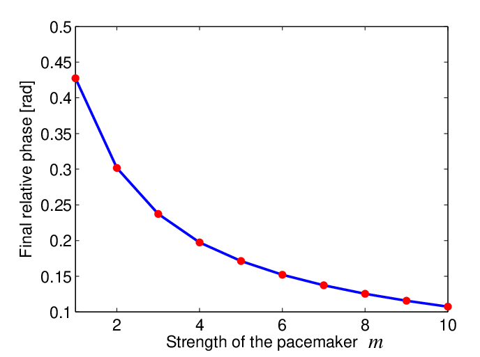
To confirm the prediction that $\xi_{i}$ can be made smaller by making the pacemaker strength stronger, we set $g_{1}=\ldots=g_{9}=g$ and simulated the network under initial phases $\varphi_{i}=\varphi_{0}+\xi_{i}$ with $\xi_{i}\in(-\pi,\,\pi)$ . Using the same $\xi_{i}$ , the maximal final relative phase when the strength of the pacemaker $g$ is made $m$ $(m=1,2,\dots,10)$ times greater is recorded and given in Fig. 3. It can be seen that the maximal final relative phase (i.e., synchronization error) decreases with the strength of the pacemaker, confirming the prediction in Theorem 6.

VI Conclusions

The exponential synchronization rate of Kuramoto oscillators is analyzed in the presence of a pacemaker. In the identical natural frequency case, we prove that synchronization to the pacemaker can be ensured even when the initial phases are not constrained in an open half-circle, which improves the existing results in the literature. Then we derive a lower bound on the exponential synchronization rate, which is proven an increasing function of the pacemaker strength, but may be an increasing or decreasing function of the local coupling strength. In the non-identical natural frequency case, a similar conclusion is obtained on phase locking. In this case, we also prove that relative phases (synchronization error) can be made arbitrarily small by making the pacemaker strength strong enough. The results are independent of oscillator numbers in the network and are confirmed by numerical simulations.

References

[1] Y. Kuramoto. Self-entrainment of a population of coupled non-linear oscillators. Int. Symp. Math. Problems Theoret. Phys., Lecture Notes Phys., 39:420–422, 1975.
[2] J. Acebrón, L. Bonilla, C. Vicente, F. Ritort, and R. Spigler. The Kuramoto model: A simple paradigm for synchronization phenomena. Rev. Mod. Phys., 77:137–185, 2005.
[3] N. Chopra and M. Spong. On exponential synchronization of Kuramoto oscillators. IEEE Trans. Autom. Control, 54:353–357, 2009.
[4] L. Scardovi, A. Sarlette, and R. Sepulchre. Synchronization and balancing on the n-torus. Syst. Control Lett., 56:335–341, 2007.
[5] M. Verwoerd and O. Mason. Global phase-locking in finite populations of coupled oscillators. SIAM J. Appl. Dyn. Syst., 7:134–160, 2008.
[6] A. Papachristodoulou and A. Jadbabaie. Synchronization in oscillator networks: switching topologies and non-homogeneous delays. In Proc. 49th IEEE Conf. Decision Control, pages 5692 –5697, Spain, 2005.
[7] J. Rogge and D. Aeyels. Stability of phase locking in a ring of undirectionally coupled oscillators. J. Phys. A: Math. Gen., 37:11135–11148, 2004.
[8] D. Klein, E. Lalish, and K. Morgansen. On controlled sinusoidal phase coupling. In Proc. Amer. Control Conf., pages 616–622, USA, 2009.
[9] A. Jadbabaie, N. Motee, and M. Barahona. On the stability of the Kuramoto model of coupled nonlinear oscillators. In Proc. Amer. Control Conf., pages 4296–4301, USA, 2004.
[10] Z. Lin, B. Francis, and M. Maggiore. State agreement for continuous-time coupled nonlinear systems. SIAM J. Control Optim., 46:288–307, 2007.
[11] A. Papachristodoulou, A. Jadbabaie, and U. Münz. Effects of delay in multi-agent consensus and oscillator synchronization. IEEE Trans. Autom. Control, 55:1471–1477, 2010.
[12] F. Dörfler and F. Bullo. Synchronization and transient stability in power networks and non-uniform Kuramoto oscillators. Submitted to IEEE Trans. Autom. Control, available on line:arXiv:0910.5673v4, 2011.
[13] P. DeLellis, M. di Bernardo, and M. Porfiri. Pinning control of complex networks via edge snapping. Chaos, 21:033119, 2011.
[14] L. M. Childs and S. H. Strogatz. Stability diagram for the forced Kuramoto model. Chaos, 18:043128, 2008.
[15] Y. Q. Wang and F. J. Doyle III. On influences of global and local cues on the rate of synchronization of oscillator networks. Automatica, 47:1236–1242, 2011.
[16] E. Herzog. Neurons and networks in daily rhythms. Nat. Rev. Neurosci., 8:790–802, 2007.
[17] H. Kopetz and W. Ochsenreiter. Clock synchronization in distributed real-time systems. IEEE Trans. Comput., 36:933–940, 1987.
[18] H. Sakaguchi. Cooperative phenomena in coupled oscillator systems under external fields. Prog. Theor. Phys., 79:39–46, 1988.
[19] H. Kori and A. Mikhailov. Entrainment of randomly coupled oscillator networks by a pacemaker. Phys. Rev. Lett., 93:254101, 2004.
[20] M. Porfiri and M. di Bernardo. Criteria for global pinning-controllability of complex networks. Automatica, 44:3100–3106, 2008.
[21] O. Popovych and P. Tass. Macroscopic entrainment of periodically forced oscillatory ensembles. Prog. Biophys. Mol. Biol., 105:98–108, 2011.
[22] N. Uchida and Z. Mainen. Speed and acuracy of olfactory discrimination in the rat. Nat. Neurosci., 6:1224–1229, 2003.
[23] Y. Q. Wang, F. Nú $\rm\tilde{n}$ ez, and F. J. Doyle III. Energy-efficient pulse-coupled synchronization strategy design for wireless sensor networks through reduced idle listening. IEEE Trans. Signal Process., 2012, DOI:10.1109/TSP.2012.2205685, awailable as preprint.
[24] Y. Q. Wang, F. Nú $\rm\tilde{n}$ ez, and F. J. Doyle III. Increasing sync rate of pulse-coupled oscillators via phase response function design: theory and application to wireless networks. IEEE Trans. Control Syst. Technol., 2012, DOI:10.1109/TCST.2012.2205254, awailable as preprint.
[25] S. Strogatz. From Kuramoto to Crawford: exploring the onset of synchronization in populations of coupled oscillators. Phys. D, 143:1–20, 2000.
[26] C. Godsil and G. Royle. Algebraic graph theory. Springer, Berlin, 2001.
[27] R. Horn and C. Johnson. Matrix analysis. Cambridge University Press, London, 1985.
[28] P. Monzón and F. Paganini. Global considerations on the Kuramoto model of sinusoudally coupled oscillators. In Proc. 44th IEEE Conf. Decision Control, pages 3923 –3928, Spain, 2005.
[29] Y. Q. Wang and F. J. Doyle III. Optimal phase response functions for fast pulse-coupled synchronization in wireless sensor networks. IEEE Trans. Signal Process., 2012, DOI:10.1109/TSP.2012.2208109, available as preprint.
[30] E. Mallada and A. Tang. Synchronization of phase-coupled oscillators with arbitrary topology. In Proc. Amer. Control Conf., pages 1777 –1782, Baltimore, USA, 2010.
[31] A. Sarlette. Geometry and symmetries in coordination control. PhD thesis, Liège University, 2009.
[32] S. Chung and J. Slotine. On synchronization of coupled Hopf-Kuramoto oscillators with phase delays. In Proc. 49th IEEE Conf. Decision Control, pages 3181–3187, USA, 2010.