Balanced Modulation for Nonvolatile Memories
Abstract
This paper presents a practical writing/reading scheme in nonvolatile memories, called balanced modulation, for minimizing the asymmetric component of errors. The main idea is to encode data using a balanced error-correcting code. When reading information from a block, it adjusts the reading threshold such that the resulting word is also balanced or approximately balanced. Balanced modulation has suboptimal performance for any cell-level distribution and it can be easily implemented in the current systems of nonvolatile memories. Furthermore, we studied the construction of balanced error-correcting codes, in particular, balanced LDPC codes. It has very efficient encoding and decoding algorithms, and it is more efficient than prior construction of balanced error-correcting codes.
Index Terms:
Balanced Modulation, Balanced LDPC Codes, Dynamic Reading Thresholds.I Introduction
Nonvolatile memories, like EPROM, EEPROM, Flash memory or Phase-change memory (PCM), are memories that can keep the data content even without power supply. This property enables them to be used in a wide range of applications, including cellphones, consumers, automotive and computers. Many research studies have been carried out on nonvolatile memories because of their unique features, attractive applications and huge marketing demands.
An important challenge for most nonvolatile memories is data reliability. The stored data can be lost due to many mechanisms, including cell heterogeneity, programming noise, write disturbance, read disturbance, etc. [2, 15]. From a long-term view, the change in data has an asymmetric property. For example, the stored data in flash memories is represented by the voltage levels of transistors, which drift in one direction because of charge leakage. In PCM, another class of nonvolatile memories, the stored data is determined by the electrical resistance of the cells, which drifts due to thermally activated crystallization of the amorphous material [21]. All these mechanisms make the errors in nonvolatile memories be heterogeneous, asymmetric, time dependent and unpredictable. These properties bring substantial difficulties to researchers attempting to develop simple and efficient error-correcting schemes.
To date, existing coding schemes for nonvolatile memories commonly use fixed thresholds to read data. For instance, in flash memories, a threshold voltage level is predetermined; when reading data from a cell, it gets ‘1’ if the voltage level is higher than , and otherwise it gets ‘0’. To increase data reliability, error-correcting codes such as Hamming code, BCH code, Reed-Solomon code and LDPC code are applied in nonvolatile memories to combat errors. Because of the asymmetric feature of nonvolatile memories, a fixed threshold usually introduces too many asymmetric errors after a long duration [14], namely, the number of errors is usually much larger than the number of errors. To overcome the limitations of fixed thresholds in reading data in nonvolatile memories, dynamic thresholds are introduced in this paper. To better understand this, we use flash memories for illustration, see Fig. 1. The top figure is for newly written data, and the bottom figure is for old data that has been stored for a long time . In the figures, assume the left curve indicates the voltage distribution for bit ‘0’ (a bit ‘0’ is written during programming) and the right curve indicates the voltage distribution for bit ‘1’. At time (the moment after programming), it is best to set the threshold voltage as , for separating bit ‘1’ and ‘0’. But after a period of time, the voltage distribution will change. In this case, is no longer the best choice, since it will introduce too many errors. Instead, we can set the threshold voltage as (see the second plot in the figure), to minimize the error probability. This also applies to other nonvolatile memories, such as PCMs.

Although best dynamic reading thresholds lead to much less errors than fixed ones, certain difficulties exist in determining their values at a time . One reason is that the accurate level distributions for bit ‘1’ and ‘0’ at any the current time are hard to obtain due to the lack of time records, the heterogeneity of blocks, and the unpredictability of exceptions. Another possible method is to classify all the cell levels into two groups based on unsupervised clustering and then map them into ‘1’s and ‘0’s. But when the border between bit ‘1’s and ‘0’s becomes fuzzy, mistakes of clustering may cause significant number of reading errors. In view of these considerations, in this paper, we introduce a simple and practical writing/reading scheme in nonvolatile memories, called balanced modulation, which is based on the construction of balanced codes (or balanced error-correcting codes) and it aims to minimize the asymmetric component of errors in the current block.
Balanced codes, whose codewords have an equal number of s and s, have been studied in several literatures. Knuth, in 1986, proposed a simple method of constructing balanced codes [10]. In his method, given an information word of -bits ( is even), the encoder inverts the first bits such that the modified word has an equal number of s and s. Knuth showed that such an integer always exists, and it is represented by a balanced word of length . Then a codeword consists of an -bit prefix word and an -bit modified information word. For decoding, the decoder can easily retrieve the value of and then get the original information word by inverting the first bits of the -bit information word again. Knuth’s method was later improved or modified by many researchers [1, 17, 19, 9]. Based on balanced codes, we have a scheme of balanced modulation. It encodes the stored data as balanced codewords; when reading data from a block, it adjusts the reading threshold dynamically such that the resulting word to read is also balanced (namely, the number of 1s is equal to the number of 0s) or approximately balanced. Here, we call this dynamic reading threshold as a balancing threshold.
There are several benefits of applying balanced modulation in nonvolatile memories. First, it increases the safety gap of s and s. With a fixed threshold, the safety gap is determined by the minimum difference between cell levels and the threshold. With balanced modulation, the safety gap is the minimum difference between cell levels for and those for . Since the cell level for an individual cell has a random distribution due to the cell-programming noise [3, 11], the actual value of the charge level varies from one write to another. In this case, balanced modulation is more robust than the commonly used fixed-threshold approach in combating programming noise. Second, as we discussed, balanced modulation can is a very simple solution that minimizes the influence of cell-level drift. It was shown in [4] that cell-level drift in flash memories introduces the most dominating errors. Third, balanced modulation can efficiently reduce errors introduced by some other mechanisms, such as the change of external temperatures and the current leakage of other reading lines, which result in the shift of cell levels in a same direction. Generally, balanced modulation is a simple approach that minimizes the influence of noise asymmetries, and it can be easily implemented on current memory devices without hardware changes. The balanced condition on codewords enables us to select a much better threshold dynamically than the commonly used fixed threshold when reading data from a block.
The main contributions of the paper are
- 1.
We study balanced modulation as a simple, practical and efficient approach to minimize asymmetric component of errors in nonvolatile memories.
- 2.
A new construction of balanced error-correcting codes, called balanced LDPC code, is introduced and analyzed, which has a higher rate than prior constructions.
- 3.
We investigate partial-balanced modulation, for its simplicity of constructing error-correcting codes, and then we extend our discussions from binary cells to multi-level cells.
II Scope of This Paper
II-A Performance and Implementation
In the first part of this paper, including Section III, Section IV and Section V, we focus on the introduction and performance of balanced modulation. In particular, we demonstrate that balanced modulation introduces much less errors than the traditional approach based on fixed thresholds. For any cell-level distributions, the balancing threshold used in balanced modulation is suboptimal among all the possible reading thresholds, in the term of total number of errors. It enables balanced modulation to be adaptive to a variety of channels characters, hence, it makes balanced modulation applicable for most types of nonvolatile memories. Beyond storage systems, balanced modulation can also be used in optimal communication, where the strength of received signals shifts due to many factors like the transmitting distance, temperature, etc.
A practical and very attractive aspect of balanced modulation is that it can be easily implemented in the current systems of nonvolatile memories. The only change is that, instead of using a fixed threshold in reading a binary vector, it allows this threshold to be adaptive. Fortunately, this operation can be implemented physically, making the process of data reading reasonably fast. In this case, the reading process is based on hard decision.
If we care less about reading speed, we can have soft-decision decoding, namely, reading data without using a threshold. We demonstrate that the prior knowledge that the stored codeword is balanced is very useful. It helps us to better estimate the current cell-level distributions, hence, resulting in a better performance in bit error rate.
II-B Balanced LDPC Code
Balanced modulation can efficiently reduce bit error rate when reading data from a block. A further question is how to construct balanced codes that are capable of correcting errors. We call such codes balanced error-correcting codes. Knuth’s method cannot correct errors. In [18], van Tilborg and Blaum presented a family of balanced binary error-correcting codes. The idea is to consider balanced blocks as symbols over an alphabet and to construct error-correcting codes over that alphabet by concatenating blocks of length each. Due to the constraint in the code construction, this method achieves only moderate rates. Error-correcting balanced codes with higher rates were presented by Al-Bassam and Bose in [1], however, their construction considers only the case that the number of errors is at most . In [12], Mazumdar, Roth, and Vontobel studied linear balancing sets, namely, balancing sets that are linear subspaces , which are applied in obtaining coding schemes that combine balancing and error correction. Recently, Weber, Immink and Ferreira extent Knuth’s method to let it equipped with error-correcting capabilities [20]. Their idea is to assign different error protection levels to the prefix and modified information word in Knuth’s construction. So their construction is a concatenation of two error-correct codes with different error correcting capabilities. In Section VI, we introduce a new construction of balanced error-correcting codes, which is based on LDPC code, so called balanced LDPC code. Such a construction has a simple encoding algorithm and its decoding complexity based on message-passing algorithm is asymptotically equal to the decoding complexity of the original (unbalanced) LDPC code. We demonstrate that balanced LDPC code has error-correcting capability very close to the original (unbalanced) LDPC code.
II-C Partial-Balanced Modulation and Its Extension
Our observation is that the task of constructing efficient balanced error-correcting codes with simple encoding and decoding algorithms is not simple, but it is much easier to construct error-correcting codes that are partially balanced, namely, only a certain segment (or subsequence) of each codeword is balanced. Motivated by this observation, we propose a variant of balanced modulation, called partial-balanced modulation. When reading from a block, it adjusts the reading threshold such that the segment of the resulting word is balanced. Partial-balanced modulation has a performance very close to that of balanced modulation, and it has much simpler constructions of error-correcting codes than balanced modulation. Another question that we address in the third part is how to extend the scheme of balanced modulation or partial-balanced modulation to be used in nonvolatile memories with multi-level cells. Details will be provided in Section VII and Section VIII.
III Balanced Modulation

For convenience, we consider different types of nonvolatile memories in the same framework where data is represented by cell levels, such as voltages in flash memories and resistance in phase-change memories. The scheme of balanced modulation is sketched in Fig. 2. It can be divided into two steps: programming step and reading step.
(1) In the programming step, we encode data based a balanced (error-correcting) code. Let denote the dimension of the code and denote the number of cells in a block, then given a message , it is mapped to a balanced codeword such that where is the Hamming weight of .
(2) In the reading step, we let be the current levels of the cells to read. A balancing threshold is determined based on such that the resulting word, denoted by , is also balanced, namely, . For each , if and only if , otherwise . By applying the decoder of the balanced (error-correcting) code, we get a binary output , which is the message that we read from the block.

Let us intuitively understanding the function of balanced modulation based on the demonstration of Fig. 3, which depicts the cell-level distributions for those cells that store or . Given a reading threshold , we use denote the number of errors and use denote the number of errors, as the tails marked in the figure. Then
We are ready to see
where is the Hamming weight of .
According to the definition, a balancing threshold is the one that makes being balanced, hence,
i.e., a balancing threshold results in the same number of errors and errors.
We define as the total number of errors based on a reading threshold , then
If the cell-level distributions for those cells that store and those cells that store are known, then the balancing threshold may not be the best reading threshold that we can have, i.e., may not be minimized based on the balancing threshold. Let denote the balancing threshold, as a comparison, we can have an optimal threshold , which is defined by
Unfortunately, it is almost impossible for us to know the cell-level distributions for those cells that store and those cells that store without knowing the original word . From this sense, the optimal threshold is imaginary. Although we are not able to determine , the following result shows that the balancing threshold has performance comparable to that of . Even in the worst case, the number of errors introduced based on is at most two times that introduced by , implying the suboptimality of the balancing threshold .
Theorem 1.
Given any balanced codeword and cell-level vector , we have
Proof.
Given the balancing threshold , the number of errors equals the number of errors, hence, the total number of errors is
If , the number of errors . Therefore,
Similarly, if , by considering only errors, we get the same conclusion. ∎
Now we compare the balancing threshold with a fixed threshold, denoted by . As shown in Fig. 3, if we set the reading threshold as fixed , then it will introduce much more errors then the balancing threshold. Given a fixed threshold , after a long duration, we can characterize the storage channel as a binary asymmetric channel, as shown in Fig. 4(a), where . Balanced modulation is actually a process of modifying the channel to make it being symmetric. As a result, balanced modulation results in a binary symmetric channel with crossover probability such that . When , it has . In this case, the bit error rate is reduced from to , where .

IV Bit-Error-Rate Analysis
To better understand different types of reading thresholds as well as their performances, we study them from the expectation (statistical) perspective. Assume that we write bits (including ones) into a block at time , let denote the probability density function (p.d.f.) of the cell level at time that stores a bit , and let denote the p.d.f. of the cell level at time that stores . Then at time , the bit error rate of the block based on a reading threshold is given by
According to our definition, a balancing threshold is chosen such that , i.e., the number of errors is equal to the number of errors. As the block length becomes sufficiently large, we can approximate as and approximate as . So when is large, we approximately have
Differently, an optimal reading threshold is the one that minimizes the total number of errors. When is large, we approximately have
When and are continuous functions, the solutions of are
That means is one of the intersections of and or one of the infinity points.
Generally, and are various for different nonvolatile memories and different blocks, and they have different dynamics over time. It is not easy to find a perfect model to characterize and , but there are two trends about them in timescale. The change of a cell level can be treated as a superposition of these two trends. First, due to cell-level drift, the difference between the means of and becomes smaller. Second, due to the existence of different types of noise and disturbance, their variances increases over time. To study the performance of balanced modulation, we consider both of the effects separately in some simple scenarios.
Example 1.
Let and , as illustrated in Fig. 5. We assume that the fixed threshold is , which satisfies .

In the above example, the cell-level distribution corresponding to bit ‘1’ drifts but its variance does not change. We have
At time , the bit error rate based on a reading threshold is
where .
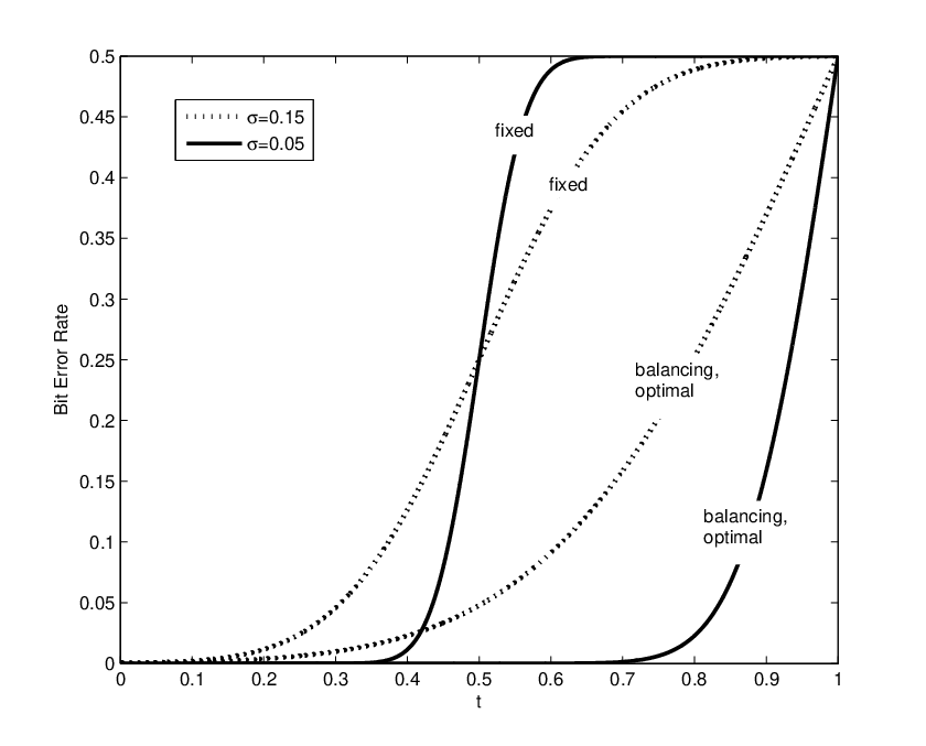
For different selections of reading thresholds, is plotted in Fig. 6. It shows that the balancing threshold and the optimal threshold have the same performance, which is much better than the performance of a fixed threshold. When cell levels drift, balanced modulation can significantly reduce the bit error rate of a block.
Example 2.
Let and , as illustrated in Fig. 7. We assume that the fixed threshold is , which satisfies .

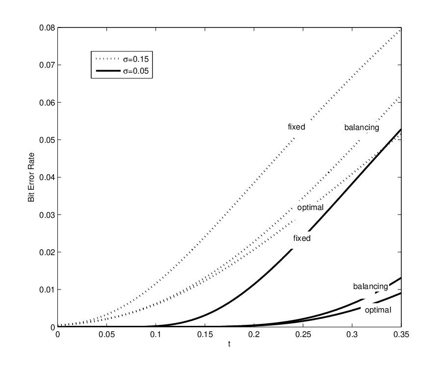
In this example, the variance of the cell-level distribution corresponding to bit ‘1’ increases as the time increases. We have
At time , the bit error rate based on a threshold is
which is plotted in Fig. 8 for different thresholds. It shows that balancing thresholds introduce much less errors than fixed thresholds when bit ‘1’ and ‘0’ have different reliability (reflected by their variances), although they introduce slightly more errors than optimal thresholds.
In practice, the cell-level distributions at a time are much more complex than the simple Gaussian distributions, and the errors introduced are due to many complex mechanisms. However, the above analysis based two simple models are still useful, because they reflect the trends of the cell level changes, which is helpful for analyzing the time-dependent errors in nonvolatile memories.
V Implementation
Balanced modulation can be easily implemented on the current architecture of nonvolatile memories. The process described in the previous sections can be treated as a hard decision approach, where a reading threshold is selected to separate all the cell levels as zeros and ones. In this section, we discuss a few methods of determining balancing thresholds quickly, as well as their implementations in nonvolatile memories. Furthermore, we discuss soft decision implementation of balanced modulation, namely, we do not read data based on a reading threshold, and the decoder can get access into all the cell levels (cell-level vector ) directly. In this case, we want to know how the prior information that the stored codeword is balanced can help us to increase the success rate of decoding.
V-A Balancing Threshold for Hard Decision
Given a block of cells, assume their current levels are . Our problem is to determine a threshold such that there are cells or approximately cells will be read as ones. A trivial method is to sort all the cell levels in the decreasing order such that . Then is our desired balancing threshold. The disadvantage of this method is that it needs computational time, which may slow down the reading speed when is large. To reduce the reading time, we hope that the balancing threshold can be controlled by hardware.
Half-interval search is a simple approach of determining the balancing threshold. Assume it is known that is with . First, we set the reading threshold as , based on which a simple circuit can quickly detect the number of ones in the resulting word, denoted by . If , we reset the interval as . If , we reset the interval as . Then we repeat this procedure until we get a reading threshold such that or for a reading precision .
V-B Relaxed Balancing Threshold
Half-interval search is an iterative approach of determining the balancing threshold such that the resulting word is well balanced. To further reduce the reading time, we can relax the constraint on the weight of the resulting word, namely, we can let the number of ones in the resulting word be approximately , instead of accurately .
For instance, we can simply set the balancing threshold as
Obviously, such reflects the cell-level drift and it can be easily implemented by a simple circuit.
More precisely, we can treat as the first-order approximation, in this way, we write as
where is a constant depending on the noise model of memory devices.
V-C Prior Probability for Soft Decision
Reading data based on hard decision is preferred in nonvolatile memories, regarding to its advantages in reading speed and computational complexity compared to soft decision decoding. However, in some occasions, soft decision decoding is still useful for increasing the decoding success rate. We demonstrate that the prior knowledge that the stored codewords are balanced can help us to better estimate the cell-level probability distributions for or . Hence, it leads to a better soft decoding performance.
We assume that given a stored bit, either or , its cell level is Gaussian distributed. (We may also use some other distribution models according to the physical properties of memory devices, and our goal is to have a better estimation of model parameters). Specifically, we assume that the cell-level probability distribution for is and the cell-level probability distribution for is . Since the codewords are balanced, the probability for a cell being or is equal. So we can describe cell levels by a Gaussian Mixture Model. Our goal is to find the maximum likelihood based on the cell-level vector , namely, the parameters that maximize
Expectation-Maximization (EM) algorithm is an iterative method that can easily find the maximum likelihood . The EM iteration alternates between performing an expectation (E) step and a maximization (M) step. Let be the codeword stored in the current block, and let be the estimation of the parameters in the th iteration. In the E-step, it computes the probability for each cell being or based on the current estimation of the parameters, namely, for all , it computes
In the M-step, it computes parameters maximizing the likelihood with given the probabilities obtained in the E-step. Specifically, for ,
These estimations of parameters are then used to determine the distribution of in the next E-step.
Assume are the maximum-likelihood parameters, based on which we can calculate the log-likelihood for each variable , that is
where is the probability density function. Based on the log-likelihood of each variable , some soft decoding algorithms can be applied to read data, including message-passing algorithms [13], linear programming [6], etc. It will be further discussed in the next section for decoding balanced LDPC code.
VI Balanced LDPC Code
Balanced modulation can significantly reduce the bit error rate of a block in nonvolatile memories, but error correction is still necessary. So we study the construction of balanced error-correcting codes. In the programming step, we encode the information based on a balanced error-correcting code and write it into a block. In the reading step, the reading threshold is adjusted such that it yields a balanced word, but probably erroneous. Then we pass this word to the decoder to further retrieve the original information.
VI-A Construction
In this section, we introduce a simple construction of balanced error-correcting codes, which is based on LDPC codes, called balanced LDPC code. LDPC codes, first introduced by Gallager [7] in 1962 and rediscovered in 1990s, achieve near Shannon-bound performances and allow reasonable decoding complexities. Our construction of balanced LDPC code is obtained by inverting the first bits of each codeword in a LDPC code such that the codeword is balanced, where is different for different codewords. It is based on Knuth’s observation [10], that is, given an arbitrary binary word of length with even, one can always find an integer with such that by inverting the first bits the word becomes balanced. Different from the current construction in [20], where is stored and protected by a lower-rate balanced error-correcting codes (the misdecoding of may lead to catastrophic error propagation in the information word), we do not store in our construction. The main idea is that certain redundancy exists in the codewords of LDPC codes that enables us to locate or at last find a small set that includes with a very high probability, even some errors exist in the codewords. It is wasteful to store the value of with a lower-rate balanced error-correcting code. As a result, our construction is more efficient than the recent construction proposed in [20].

Let be the message to encode and its length is , according to the description above, the encoding procedure consists of two steps, as shown in Fig. 9:
- 1.
Apply an LDPC code to encode the message into a codeword of length , denoted by , where is the generator matrix of .
- 2.
Find the minimal integer in such that inverting the first bits of results in a balanced word
where denotes a run of bits and bits . Then we denote as . This word is a codeword of the resulting balanced LDPC code, denoted by .
We see that a balanced LDPC code is constructed by simply balancing the codewords of a LDPC code, which is called the original LDPC code. Based on the procedure above we can encode any message of length into a balanced codeword of length . The encoding procedure is very simple, but how to decode a received word? Now, we focus on the decoding of this balanced LDPC code. Let be an erroneous word received by the decoder, then the output of the maximum likelihood decoder is
where is the distance between and depending on the channel, for instance, Hamming distance for binary symmetric channels.
The balanced code is not a linear code, so the constraint is not easy to deal with. A simpler way is to think about the codeword that corresponds to . By inverting the first bits of with , we can get a set of words of size , namely,
in which
for all . Then there exists an such that
The output of the maximum likelihood decoder is
subject to is the minimum integer that makes being balanced.
If we ignore the constraint that has to be the minimum integer, then the output of the decoder is the codeword in that has the minimum distance to . Fig. 10 provides a simple demonstration, where the solid circles are for the codewords of the LPDC code , the triangles are for the words in that are connected by lines. Our goal is to find the solid circle that is the closest one to the set of triangles. It is different from traditional decoding of linear codes whose goal is to find the closest codeword to a single point.

VI-B An Extreme Case
LDPC codes achieve near Shannon bound performances. A natural question is whether balanced LDPC codes hold this property. Certain difficulties exist in proving it by following the method in [8] (section 2 and section 3), since balanced LDPC codes are not linear codes and the distance distributions of balanced LDPC codes are not easy to characterize. Fortunately, this statement looks correct because if the first bits of a codeword have been inverted (we assume that the interger is unknown), then the codeword can be recovered with only little cost, i.e., a very small number of additional redundant bits.
Let us consider the ensemble of an parity-check matrix given by Gallager [8], which has ones in each column, ones in each row, and zeros elsewhere. According to this construction, the matrix is divided into submatrices, each containing a single in each column. All the submatrices are random column permutations of a matrix that has a single one in each column and ones in each row. As a result, we have LDPC codes.
Theorem 2.
Given a codeword of an LDPC code, we get
by inverting the first bits of with . Let be the error probability that cannot be correctly recovered from if is unknown. As ,
for any integers and .
Proof.
Let be the parity-check matrix of the LDPC code, and let
for all .
We can recover from if and only if
for all and .
Hence,
Let us first consider the case of . We have if and only if
where
So is equivalent to
As we described, is constructed by submatrices, namely, we can write as
Let be one of the submatrices of , then contains a single one in each columns and ones in each row. And it satisfies
i.e., in each row of , there are even number of ones from the th column to the th column.
According to the construction of LDPC codes,
So we can use to denote .
First, we consider the case that is even. In this case,
Hence, without loss of generality, we can assume that .
It is easy to see that only if is even. Assume that the one in the first column of is in the th row, and let be the number of ones in the th row from the first columns. Then we can get
where if or .
If , then .
If , then
Iteratively, we can prove that
Similar as above, when , we can get
Finally, we have
So if is even, as , .
If is odd, in each row, there exists at least one in the last elements. As a result, . Using a same idea as above, we can also prove that as , .
So the statement in the theorem is true for any rate . This completes the proof. ∎
The above theorem considers an extreme case that if the codeword of a balanced LDPC code does not have errors, then we can recover the original message with little cost of redundancy. It implies that balanced LDPC codes may achieve almost the same rates as the original unbalanced LDPC codes. In the following subsections, we discuss some decoding techniques for binary erasure channels and binary symmetric channels. Simulation results on these channels support the above statement.
VI-C Decoding for Erasure Channels
In this subsection, we consider binary erasure channels (BEC), where a bit ( or ) is either successfully received or it is deleted, denoted by “”. Let be a word received by a decoder after transmitting a codeword over a BEC. Then the key of decoding is to determine the value of the integer such that can be obtained by inverting the first bits of a codeword in .
A simple idea is to search all the possible values of , i.e., we decode all the possible words separately and select the best resulting codeword that satisfies all the constraints as the final output. This idea is straightforward, but the computational complexity of the decoding increases by a factor of , which is not acceptable for most practical applications.
Our observation is that we might be able to determine the value of or at least find a feasible set that includes , based on the unerased bits in . For example, given , assume that one parity-check constraint is
If all are observed (not erased), then we can have the following statement about :
(1) If , then
(2) If , then
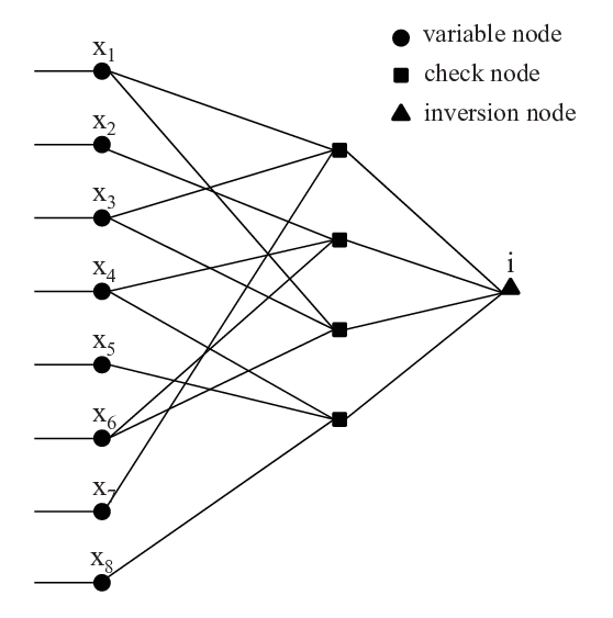
By combining this observation with the message-passing algorithm, we get a decoding algorithm for balanced LDPC codes under BEC. Similar as the original LDPC code, we present a balanced LDPC code as a sparse bipartite graph with variable nodes and check nodes, as shown in Fig. 11. Additionally, we add an inversion node for representing the value or the feasible set of . Let us describe a modified message-passing algorithm on this graph. In each round of the algorithm, messages are passed from variable nodes and inversion nodes to check nodes, and then from check nodes back to variable nodes and inversion nodes.
We use denote the feasible set consisting of all possible values for the integer , called inversion set. At the first round, we initialize the th variable node and initialize the inversion set as . Then we pass message and update the graph iteratively. In each round, we do the following operations.
(1) For each variable node , if its value is in , it sends to all its check neighbors. If and any incoming message is or , it updates as and sends to all its check neighbors. If and all the incoming messages are , it sends to all its check neighbors.
(2) For each check node , assume the messages from its variable neighbors are , where are the indices of these variable nodes s.t. . Then we define
If all the incoming messages are in , then we update in the following way: If , we update as ; otherwise, we update as . In this case, this check node is no longer useful, so we can remove this check node from the graph.
(3) For each check node , if there are exactly one incoming message from its variable neighbor which is and all other incoming messages are in , we check whether or . If , then the check node sends the XOR of the other incoming messages except to . If , then the check node sends the XOR of the other incoming messages except plus one to . In this case, the check node is also no longer useful, so we can remove this check node from the graph.
The procedure above continues until all erasures are filled in, or no erasures are filled in the current iteration. Different from the message-passing decoding algorithm for LDPC codes, where in each iteration both variable nodes and check nodes are processed only once, here, we process variable nodes once but check nodes twice in each iteration. If all erasures are filled in, is the binary vector labeled on the variable nodes. In this case, if , then is the only element in , and we can get by calculating
If there are still some unknown erasures, we enumerate all the possible values in for the integer . Usually, is small. For a specific , it leads to a feasible solution if
(1) Given , with the message-passing procedure above, all the erasures can be filled in.
(2) is balanced, namely, the numbers of ones and zeros are equal for the variable nodes.
(3) Let . Then is the minimal integer in subject to is balanced.
We say that a word with erasures is uniquely decodable if and only if there exists that leads to a feasible solution, and for all such integers they result in the unique solution . The following simple example is provided for the purpose of demonstrating the decoding process.
Example 3.
Based on Fig. 11, we have a codeword , which is transmitted over an erasure channel. We assume that the received word is .
In the first round of the decoding, we have
Considering the nd check node, we can update as
Considering the nd check node, we can continue updating as
Based on (3), we can fill for the th and th variable nodes. Finally, we get and .

Regarding to the decoding algorithm described above, there are two important issues that need to consider, including the decoding complexity of the algorithm and its performance. First, the decoding complexity of the algorithm strongly depends on the size of when it finishes iterations. Fig. 12 simulates the average size of the inversion set for decoding three balanced LDPC codes. It shows that when the crossover probability is lower than a threshold, the size of is smaller than a constant with a very high probability. In this case, the decoding complexity of the balanced LDPC code is very close to the decoding complexity of the original unbalanced LDPC code.

Another issue is about the performance of the decoding algorithm for balanced LDPC codes. In particular, we want to figure out the cost of additional redundancy in correcting the inversion of the first bits when is unknown. In Fig. 13, it presents the word error rate of balanced LDPC codes and the corresponding original unbalanced LDPC codes for different block lengths. It is interesting to see that as the block length increases, the balanced LDPC codes and the original unbalanced LDPC codes have almost the same performance, that is, the cost of correcting the inversion of the first bits is ignorable.
VI-D Decoding for Symmetric Channels
In this subsection, we study and analyze the decoding of balanced LDPC codes for symmetric channels, including binary symmetric channels (BSC) and AWGN (Additive White Gaussian Noise) channels. Different from binary erasure channels (BEC), here we are not able to determine a small set that definitely includes the integer . Instead, we want to figure out the most possible values for . Before presenting our decoding algorithm, we first introduce belief propagation algorithm for decoding LDPC codes.
Belief propagation [13], where messages are passed iteratively across a factor graph, has been widely studied and recommended for the decoding of LDPC codes. In each iteration, each variable node passes messages (probabilities) to all the adjacent check nodes and then each check node passes messages (beliefs) to all the adjacent variable nodes. Specifically, let be the message passed from a variable node to a check node at the th round of the algorithm, and let be the message from a check node to a variable node . At the first round, is the log-likelihood of the node conditioned on its observed value, i.e., for variable and its observation . This value is denoted by . Then the iterative update procedures can be described by the following equations
where is the set of check nodes that connect to variable node and is the set of variable nodes that connect to check node . In practice, the belief-propagation algorithm stops after a certain number of iterations or until the passed likelihoods are close to certainty. Typically, for a BSC with crossover probability , the log-likelihood for each variable node is a constant depending on . Let be the variable on and let be its observation, then
Let us consider the decoding of balanced LDPC codes. Assume is a codeword of a balanced LDPC code, obtained by inverting the first bits of a codeword in a LDPC code . The erroneous word received by the decoder is for an alphabet . For example, for BSC channels, and for AWGN channels. Here, we consider a symmetric channel, i.e., a channel for which there exists a permutation of the output alphabet such that (1) , and (2) for all , where is the probability of observing when the input bit is .
The biggest challenge of decoding a received word is lacking of the location information about where the inversion happens, i.e., the integer . We let
for all . A simple idea is to search all the possibilities for the integer from to , i.e, decoding all the words
separately. Assume their decoding outputs based on belief propagation are
then the final output of the decoder is such that is maximized. The drawback of this method is its high computational complexity, which is about times the complexity of decoding the original unbalanced LDPC code. To reduce computational complexity, we want to estimate the value of in a simpler and faster way, even sacrificing a little bit of performance on bit error rate.
The idea is that when we are using belief propagation to decode a group of words , some information can be used to roughly compare their goodness, namely, their distances to the nearest codewords. To find such information, given each word (here, we denote it as for simplicity), we run belief propagation for rounds (iterations), where is very small, e.g., . There are several ways of estimating the goodness of , and we introduce one of them as follows.
Given a word , we define
where is the set of all the variable nodes, is the set of neighbors of a check node , and is the message passed from a variable node to a check node at the th round of the belief-propagation algorithm. Roughly, is a measurement of the number of correct parity checks for the current assignment in belief propagation (after iterations). For instance,
for a binary symmetric channel. In this expression, is a constant, is the number of redundancies, and is the number of ones in , i.e., the number of unsatisfied parity checks.
Generally, the bigger is, the more likely is. So we can get the most likely by calculating
Then we decode as the final output. However, the procedure requires to calculate with . The following theorem shows that the task of computing all with can be finished in linear time if is a small constant.
Theorem 3.
The task of computing all with can be finished in linear time if is a small constant.
Proof.
First, we calculate . Based on the belief-propagation algorithm described above, it can be finished in time. In this step, we save all the messages including , , for all and .
When we calculate , the only change on the inputs is , where is the first variable node (the sign of is flipped). As a result, we do not have to calculate all , , for all and . Instead, we only need to update those messages that are related with . It needs to be noted that the number of messages related to has an exponential dependence on , so the value of should be small. In this case, based on the calculation of , can be calculated in a constant time. Similarly, each of with can be obtained iteratively in a constant time.
Based on the process above, we can compute all with in time. ∎
To increase the success rate of decoding, we can also create a set of most likely values for , denoted by . consists of at most local maximums with the highest values of . Here, we say that is a local maximum if and only if
Note that , where is the global maximum as defined above. If , for all , we decode separately and choose the output with the maximum likelihood as the final output of the decoder. It is easy to see that the the above modified belief-propagation algorithm for balanced LDPC codes has asymptotically the same decoding complexity as the belief-propagation algorithm for LDPC codes, that is, .

In Fig. 14, it shows the performance of the above algorithm for decoding balanced LDPC codes under BSC and the performance of belief propagation algorithm for the original LDPC codes. From which, we see that when and , the performance gap between balanced LDPC code and unbalanced LDPC code is very small. This comparison implies that the cost of correcting the inversion of the first bits (when is unknown) is small for LDPC codes.
Let us go back the scheme of balanced modulation. The following examples give the log-likelihood of each variable node when the reading process is based on hard decision and soft decision, respectively. Based on them, we can apply the modified propagation algorithm in balanced modulation.
Example 4.
If the reading process is based on hard decision, then it results in a binary symmetric channel with crossover probability . In this case, let be the observation on a variable node , the log-likelihood for is
Example 5.
If the reading process is based on soft decision, then we can approximate cell-level distributions by Gaussian distributions, which are characterized by parameters . These parameters can be obtained based on the cell-level vector , following the steps in Subsection V-C. In this case, if the input of the decoder is , then the log-likelihood of the th variable node is
where is the current level of the th cell. If the input of the decoder is (we don’t have to care about its exact value), then the log-likelihood of the th variable node is
for all .
VII Partial-Balanced Modulation
Constructing balanced error-correcting codes is more difficult than constructing normal error-correcting codes. A question is: is it possible to design some schemes that achieve similar performances with balanced modulation and have simple error-correcting code constructions? With this motivation, we propose a variant of balanced modulation, called partial-balanced modulation. The main idea is to construct an error-correcting code whose codewords are partially balanced, namely, only a certain segment of each codeword is balanced. When reading information from a block, we adjust the reading threshold to make this segment of the resulting word being balanced or being approximately balanced.

One way of constructing partial-balanced error-correcting codes is shown in Fig. 15. Given an information vector of bits ( is even), according to Knuth’s observation [10], there exists an integer with such that inverting the first bits of results in a balanced word . Since our goal is to construct a codeword that is partially balanced, it is not necessary to present in a balanced form. Now, we use denote the binary representation of length for . To further correct potential errors, we consider as the information part and add extra parity-check bits by applying a systematic error-correcting code, like BCH code, Reed-Solomon code, etc. As a result, we obtain a codeword where is the redundancy part. In this codeword, is balanced, is not balanced.
Note that in most data-storage applications, the bit error rate of a block is usually very small. The application of modulation schemes can further reduce the bit error rate. Hence, the number of errors in real applications is usually much smaller than the block length. In this case, the total length of is smaller or much smaller than the code dimension . As the block length becomes large, like one thousand, the reading threshold determined by partial-balanced modulation is almost the same as the one determined by balanced modulation. One assumption that we made is that all the cells in the same block have similar noise properties. To make this assumption being sound, we can reorder the bits in such that the cells of storing is (approximately) randomly distributed among all the cells. Compared to balanced modulation, partial-balanced modulation can achieve almost the same performance, and its code construction is much easier (the constraints on the codewords are relaxed). In the following two examples, it compares the partial-balanced modulation scheme with the traditional one based on a fixed threshold.
Example 6.
Let us consider a nonvolatile memory with block length . To guarantee the data reliability, each block has to correct errors if the reading process is based on a fixed reading threshold. Assume primitive BCH code is applied for correcting errors, then the data rate (defined by the ratio between the number of available information bits and the block length) is
Example 7.
For the block discussed in the previous example, we assume that it only needs to correct errors based on partial-balanced modulation. In this case, we can apply primitive BCH code for correcting errors, and the data rate is
which is much higher than the one obtained in the previous example.
The reading/decoding process of partial-balanced modulation is straightforward. First, the reading threshold is adjusted such that among the cells corresponding to there are cells or approximately cells with higher levels than . Based on this reading threshold , the whole block is read as a binary word , which can be further decoded as if the total number of errors is well bounded. Then we obtain the original message by inverting the first bits of .
VIII Balanced Codes for Multi-Level Cells
In order to maximize the storage capacity of nonvolatile memories, multi-level cells (MLCs) are used, where a cell of discrete levels can store bits [3]. Flash memories with 4 and 8 levels have been used in products, and MLCs with levels have been demonstrated in prototypes. For PCMs, cells with or more levels have been in development.
The idea of balanced modulation and partial-balanced modulation can be extended to multi-level cells. For instance, if each cell has levels, we can construct a balanced code in which each codeword has the same number of s, s, s, and s. When reading data from the block, we adjust three reading thresholds such that the resulting word also has the same number of s, s, s, and s. The key question is how to construct balanced codes or partial-balanced codes for an alphabet size .
VIII-A Construction based on Rank
A simple approach of constructing balanced codes for a nonbinary case is to consider the message as the rank of its codeword among all its permutations, based on the lexicography order. If the message is , then the codeword length is the minimum integer such that and The following examples are provided for demonstrating the encoding and decoding processes.
Example 8.
Assume the message is of length and . Since , we can convert to a balanced word of length and alphabet size . Let denote the set that consists of all the balanced words of length and alphabet size . To map into a word in , we write into the decimal form and let be the rank of in based on the lexicographical order.
Let us consider the first symbol of . In , there are totally sequences starting with , or , or . Since , the first symbol in would be , then we update as , which is the rank of among all the sequences starting with .
Let us consider the second symbol of . There are totally sequences starting with , and it is larger than , so the second symbol of is .
Repeating this process, we can convert into a balanced word .
Example 9.
We use the same notations as the above example. Given , it is easy to calculate its rank in based on the lexicographical order (via enumerative source coding [5]). It is
where is the number of ’s permutations starting with , is the number of permutations starting with , …
Then from , we can get its binary representation . In [16], Ryabko and Matchikina showed that if the length of is , then we can get the message in time.
The above approach is simple and information efficient, but the encoding is not computationally fast.
VIII-B Generalizing Knuth’s Construction
An alternative approach is to generalize Knuth’s idea to the nonbinary case due to its operational simplicity. Generally, assume that we are provided a word with and , our goal is to generalize Knuth’s idea to make being balanced.
Let us consider a simple case, . Given a word , we let with denote the number of s in . To balance all the cell levels, we first balance the total number of s and s, such that . It also results in . To do this, we can treat and as an identical state and treat and as another identical state. Based on Knuth’s idea, there always exists an integer such that by operating on the first symbols (, , , ) it yields . We then consider the subsequence consisting of s and s, whose length is . By applying Knuth’s idea, we can make this subsequence being balanced. Similarly, we can also balance the subsequence consisting of s and s. Consequently, we convert any word in into a balanced word. In order to decode this word, three additional integers of length at most need to be stored, indicating the locations of having operations. The following example is constructed for the purpose of demonstrating this procedure.
Example 10.
Assume , we convert it into a balanced word with the following steps:
(1) By operating the first symbols in , it yields , where .
(2) Considering the subsequence of s and s, i.e., the underlined part in . By operating the first bit of this subsequence , it yields , where .
(3) Considering the subsequence of s and s, i.e., the underlined part in . By operating the first bit of this subsequence , it yields , which is balanced.
To recover from (the inverse process), we need to record the three integers whose binary lengths are .
It can be observed that the procedure above can be easily generalized for any with . If with , then the number of bits to store the integers (locations) is
For instance, if and , then and it requires bits to represent the locations. These bits can be stored in cells without balancing.
In fact, the above idea can be generalized for an arbitrary . For instance, when , given an binary word , there exists an integer such that has exactly s or s. Without loss of generality, we assume that it has exactly s, then we can further balance the subsequence consisting of s and s. Finally, we can get a balanced word with alphabet size . More generally, we have the following result.
Theorem 4.
Given an alphabet size with two integers and , we divide all the levels into groups, denoted by , , …, . Given any word , there exists an integer such that has exactly symbols in one of the first groups.
Proof.
Let us denote all the groups as . Given a sequence , we use denote the number of symbols in that belong to . Furthermore, we let denote the number of symbols in that belong to . It is easy to see that for all , where . We prove that that there exists such that or by contradiction. Assume this statement is not true, then either or for all . So if , we can get for all iteratively. Similarly, if , we can get for all iteratively. Both cases contradict with the fact that .
Note that the number of symbols in that belong to changes by at most if we increase by one. So if there exists such that or , there always exists an integer such that has exactly symbols in .
This completes the proof. ∎
Based on the above result, given any , we can always split all the levels into two groups and make them being balanced (the number of symbols belonging to a group is proportional to the number of levels in that group). Then we can balance the levels in each group. Iteratively, all the levels will be balanced. In order to recover the original message, it requires roughly
bits for storing additional information when is large. If we store this additional information as a prefix using a shorter balanced code, then we get a generalized construction of Knuth’s code. If we follow the steps in Section VII by further adding parity-check bits, then we get a partial-balanced code with error-correcting capability, based on which we can implement partial-balanced modulation for multiple-level cells.
Now, if we have a code that uses ‘full’ sets of balanced codewords, then the redundancy is
bits. So given an alphabet size , the redundancy of the above method is about times as high as that of codes that uses ‘full’ sets of balanced codewords. For , we list these factors as follows:
It shows that as increases, the above method becomes less information efficient. How to construct balanced codes for a nonbinary alphabet in a simple, efficient and computationally fast way is still an open question. It is even more difficult to construct balanced error-correcting codes for nonbinary alphabets.
IX Conclusion
In this paper, we introduced balanced modulation for reading/writing in nonvolatile memories. Based on the construction of balanced codes or balanced error-correcting codes, balanced modulation can minimize the effect of asymmetric noise, especially those introduced by cell-level drifts. Hence, it can significantly reduce the bit error rate in nonvolatile memories. Compared to the other schemes, balanced modulation is easy to be implemented in the current memory systems and it does not require any assumptions about the cell-level distributions, which makes it very practical. Furthermore, we studied the construction of balanced error-correcting codes, in particular, balanced LDPC codes. It has very efficient encoding and decoding algorithms, and it is more efficient than prior construction of balanced error-correcting codes.
References
- [1] S. Al-Bassam and B. Bose, “On balanced codes,” IEEE Trans. Inform. Theory, vol. 36, pp. 406–408, Mar. 1990.
- [2] R. Bez, E. Camerlenghi, A. Modelli, and A. Visconti, “Introduction to flash memory,” Proceedings of the IEEE, vol. 91, pp. 489–502, 2003.
- [3] J. E. Brewer and M. Gill, Nonvolatile Memory Technologies with Emphasis on Flash, John Wiley & Sons, Hoboken, New Jersey, 2008.
- [4] Y. Cai, E. F. Haratsch, O. Mutlu, K. Mai, “Error patterns in MLC NAND Flash memory: Measurement, characterization, and analysis,” in Proc. Design, Automation, and Test in Europe (DATE), 2012.
- [5] T. M. Cover, “Enumerative source coding,” IEEE Trans. Inform. Theory, vol. 19, no. 1, pp. 73–77, Jan. 1973.
- [6] J. Feldman, M. J. Wainwright, and D. R. Karger, “Using linear programming to decode binary linear codes”, IEEE Trans. Inform. Theory, vol. 51, pp. 954–972, Mar. 2005.
- [7] R. Gallager, “Low density parity check codes,” IRE Trans. Inform. Theory, vol. 8, no. 1, pp. 21–28, Jan. 1962.
- [8] R. Gallager, Low Density Parity Check Codes, no. 21 in Research Monograph Series. Cambridge, MA: MIT Press, 1963.
- [9] K. S. Immink and J. Weber, “Very efficient balanced codes,” IEEE Journal on Selected Areas in Communications, vol. 28, pp. 188–192, 2010.
- [10] D. E. Knuth, “Efficient balanced codes,” IEEE Trans. Inform. Theory, vol. 32, no. 1, pp. 51–53, 1986.
- [11] H. T. Lue et al., “Study of incremental step pulse programming (ISPP) and STI edge effect of BE-SONOS NAND flash,” in Proc. IEEE Int. Symp. on Reliability Physics, pp. 693–694, May 2008.
- [12] A. Mazumdar, R. M. Roth, and P. O. Vontobel, “On linear balancing sets,” in Proc. IEEE Int. Symp. Information Theory, pp. 2699–2703, 2009.
- [13] R. McEliece, D. MacKay, and J. Cheng, “Turbo decoding as an instance of Pearl’s belief propagation algorithm,” IEEE J. Sel. Areas Commun., vol. 16, no. 2, pp. 140–152, Feb. 1998.
- [14] N. Mielke, T. Marquart, N. Wu, J. Kessenich, H. Belgal, E. Schares, F. Trivedi, E. Goodness, and L. R. Nevill, “Bit error rate in NAND Flash memories,” in IEEE International Reliability Physics Symposium, pp. 9–19, 2008.
- [15] A. Pirovano, A. Redaelli, et al., “Reliability study of phase-change nonvolatile memories,” IEEE Transactions on Device and Materials Reliability, vol. 4, pp. 422–427, 2004.
- [16] B. Y. Ryabko and E. Matchikina, “Fast and efficient construction of an unbiased random sequence,” IEEE Trans. Inform. Theory, vol. 46, pp. 1090–1093, 2000.
- [17] L. G. Tallini, R. M. Capocelli, and B. Bose, “Design of some new balanced codes,” IEEE Trans. Inform. Theory, vol. 42, pp. 790–802, May 1996.
- [18] H. van Tilborg and M. Blaum, “On error-correcting balanced codes,” IEEE Trans. Inf. Theory, vol. 35, no. 5, pp. 1091–1095, Sep. 1989.
- [19] J. H. Weber and K. A. S. Immink, “Knuth’s balanced code revisited,” IEEE Trans. Inform. Theory, vol. 56, no. 4, pp. 1673–1679, Apr. 2010.
- [20] J. Weber, K. S. Immink and H. Ferreira, “Error-correcting balanced Knuth codes,” IEEE Trans. Inform. Theory, vol. 58, no. 1, pp. 82–89, 2012.
- [21] H. Wong, S. Raoux, S. Kim, J. Liang, J. P. Reifenberg, B. Rajendran, M. Asheghi, and K. E. Goodson, “Phase change memory,” Proc. IEEE, vol. 98, no. 12, pp. 2201–2227, Dec. 2010.