The Synthesis and Analysis of Stochastic Switching Circuits

Hongchao Zhou Po-Ling Loh Jehoshua Bruck ^†^†thanks: This work was supported in part by the NSF Expeditions in Computing Program under grant CCF-0832824. This paper was presented in part at IEEE International Symposium on Information Theory (ISIT), Seoul, Korea, June 2009.^†^†thanks: H. Zhou and J. Bruck are with the Department of Electrical Engineering, California Institute of Technology, Pasadena, CA, 91125. Email: hzhou@caltech.edu, bruck@caltech.edu^†^†thanks: P. Loh is with the Department of Statistics, University of California, Berkeley, CA 94720. Email: ploh@berkeley.edu

Abstract

Stochastic switching circuits are relay circuits that consist of stochastic switches called pswitches. The study of stochastic switching circuits has widespread applications in many fields of computer science, neuroscience, and biochemistry. In this paper, we discuss several properties of stochastic switching circuits, including robustness, expressibility, and probability approximation.

First, we study the robustness, namely, the effect caused by introducing an error of size $\epsilon$ to each pswitch in a stochastic circuit. We analyze two constructions and prove that simple series-parallel circuits are robust to small error perturbations, while general series-parallel circuits are not. Specifically, the total error introduced by perturbations of size less than $\epsilon$ is bounded by a constant multiple of $\epsilon$ in a simple series-parallel circuit, independent of the size of the circuit.

Next, we study the expressibility of stochastic switching circuits: Given an integer $q$ and a pswitch set $S=\{\frac{1}{q},\frac{2}{q},\dots,\frac{q-1}{q}\}$ , can we synthesize any rational probability with denominator $q^{n}$ (for arbitrary $n$ ) with a simple series-parallel stochastic switching circuit? We generalize previous results and prove that when $q$ is a multiple of $2$ or $3$ , the answer is yes. We also show that when $q$ is a prime number larger than $3$ , the answer is no.

Probability approximation is studied for a general case of an arbitrary pswitch set $S=\{s_{1},s_{2},\dots,s_{|S|}\}$ . In this case, we propose an algorithm based on local optimization to approximate any desired probability. The analysis reveals that the approximation error of a switching circuit decreases exponentially with an increasing circuit size.

Index Terms:

Stochastic Switching Circuits, Robustness, Probability Synthesis, Probability Approximation.

I Introduction

In his master’s thesis of 1938, Claude Shannon demonstrated how Boolean algebra can be used to synthesize and simplify relay circuits, establishing the foundation of modern digital circuit design [12]. Later, deterministic switches were replaced with probabilistic switches to make stochastic switching circuits, which were studied in [15]. There are a few features of stochastic switching circuits that make them very similar to neural systems. First, randomness is inherent in neural systems and it may play a crucial role in thinking and reasoning. Switching (and relaying) technique provides us a natural way of manipulating this randomness. Second, in a switching system, each switch can be treated as either a memory element or a control element for computing. This might enable creating an intelligent system where storage and computing are highly integrated. In this paper, we study stochastic switching circuits from a basic starting point with focusing on probability synthesis. We consider two-terminal stochastic switching circuits, where each probabilistic switch, or pswitch, is closed with some probability chosen from a finite set of rational numbers, called a pswitch set. By selecting pswitches with different probabilities and composing them in appropriate ways, we can realize a variety of different closure probabilities.

Formally, for a two-terminal stochastic switching circuit $C$ , the probabilities of pswitches are taken from a fixed pswitch set $S$ , and all these pswitches are open or closed independently. We use $P(C)$ to denote the probability that the two terminals of $C$ are connected, and call $P(C)$ the closure probability of $C$ . Given a pswitch set $S$ , a probability $x$ can be realized if and only if there exists a circuit $C$ such that $x=P(C)$ . Based on the ways of composing pswitches, we have series-parallel (sp) circuits and non-series-parallel (non-sp) circuits. An sp circuit consists of either a single pswitch or two sp circuits connected in series or parallel, see the circuit in Fig. 1(a) and 1(b) as examples. The circuit in Fig. 1(c) is a non-sp circuit. A special type of sp circuits is called simple-series-parallel (ssp) circuits. An ssp circuit is either a single pswitch, or is built by taking an ssp circuit and adding another pswitch in either series or parallel. For example, the circuit in Fig. 1(a) is an ssp circuit but the one in Fig. 1(b) is not.

In this paper, we first study the robustness of different stochastic switching circuits in the presence of small error perturbations. We assume that the probabilities of individual pswitches are taken from a fixed pswitch set with a given error allowance of $\epsilon$ ; that is, the error probabilities of the pswitches are bounded by $\epsilon$ . We show that ssp circuits are robust to small error perturbations, but the error probability of a general sp circuit may be amplified by adding additional pswitches. These results might help us understand why local errors do not accumulate in a natural system, and how to enhance the robustness of a system when designing a circuit.

Next, we study the problem of synthesizing desired probabilities with stochastic switching circuits. We mainly focus on ssp circuits due to their robustness against small error perturbations. Two main questions are addressed: (1) Expressibility: Given the pswitch set $S=\{\frac{1}{q},\frac{2}{q},\ldots,\frac{q-1}{q}\}$ , where $q$ is an integer, what kind of probabilities can be realized using stochastic switching circuits? And how many pswitches are sufficient to realize them? (2) Approximation: Given an arbitrary pswitch set $S$ , how can we construct a stochastic switching circuit using as a few as possible pswitches, to get a good approximation of the desired probabilities?

Refer to caption — (a) ssp circuit. $P(C)=\frac{5}{8}$ .

The study of probability synthesis based on stochastic switching circuits has widespread applications. Recently, people found that DNA molecules can be constructed that closely approximate the dynamic behavior of arbitrary systems of coupled chemical reactions [13], which leads to the field of molecular computing [2]. In such systems, the quantities of molecules involved in a reaction are often surprisingly small, and the exact sequence of reactions is determined by chance [4]. Stochastic switching circuits provide a simple and powerful tool to manipulate stochasticity in molecular systems. Comparing with combinational logic circuits, stochastic switching circuits are easier to implement using molecular reactions. Another type of applications is probabilistic electrical systems without sophisticated computing components. In such systems, stochastic switching circuits have many advantages in generating desired probabilities, including its constructive simplicity, robustness, and low cost.

The remainder of this paper is organized as follows: Section II describes related work and introduces some existing results on stochastic switching circuits. In Section III, we analyze the robustness of different kinds of stochastic switching circuits. Then we discuss the expressibility of stochastic switching circuits in Section IV and probability approximation in Section V, followed by the conclusion in Section VI.

II Related Works and Preliminaries

There are a number of studies related to the problem of generating desired distributions from the algorithmic perspective. This problem dates back to von Neumann [14], who considered of simulating an unbiased coin using a biased coin with unknown probability. Later, Elias [3] improved this algorithm such that the expected number of unbiased random bits generated per coin toss is asymptotically equal to the entropy of the biased coin. On the other hand, people have considered the case that the probability distribution of the tossed coin is known. Knuth and Yao [9] have given a procedure to generate an arbitrary probability using an unbiased coin. Han and Hoshi [7] have demonstrated how to generate an arbitrary probability using a general $M$ -sided biased coin. All these works aim to efficiently convert one distribution to another. However, they require computing models and may not be applicable for some simple or distributed electrical/molecular systems.

There are a number of studies focusing on synthesizing a simple physical device to generate desired probabilities. Gill [5][6] discussed the problem of generating rational probabilities using a sequential state machine. Motivated by neural computation, Jeavons et al. provided an algorithm to generate binary sequences with probability $\frac{a}{q^{n}}$ from a set of stochastic binary sequences with probabilities in $\{\frac{1}{q},\frac{2}{q},\ldots,\frac{q-1}{q}\}$ [8]. Their method can be implemented using the concept of linear feedback shift registers. Recently, inspired by PCMOS technology [1], Qian et al. considered the synthesis of decimal probabilities using combinational logic [11]. They have considered three different scenarios, depending on whether the given probabilities can be duplicated, and whether there is freedom to choose the probabilities. In contact to the foregoing contributions, we consider the properties and probability synthesis of stochastic switching circuits. Our approach is orthogonal and complementary to that of Qian and Riedel, which is based on combinational logic. Generally, each switching circuit can be equivalently expressed by a combinational logic circuit. All the constructive methods of stochastic switching circuits in this paper can be directly applied to probabilistic combinational logic circuits.

In the rest of this section, we introduce the original work that started the study on stochastic switching circuits (Wilhelm and Bruck [15]). Similar to resistor circuits [10], connecting one terminal of a switching circuit $C_{1}$ (where $P(C_{1})=p_{1}$ ) to one terminal of a circuit $C_{2}$ (where $P(C_{2})=p_{2}$ ) places them in series. The resulting circuit is closed if and only if both of $C_{1}$ and $C_{2}$ are closed, so the probability of the resulting circuit is

p_{\mathrm{series}}=p_{1}\cdot p_{2}.

Connecting both terminals of $C_{1}$ and $C_{2}$ together places the circuits in parallel. The resulting circuit is closed if and only if either $C_{1}$ or $C_{2}$ is closed, so the probability of the resulting circuit is

p_{\mathrm{parallel}}=1-(1-p_{1})(1-p_{2})=p_{1}+p_{2}-p_{1}p_{2}.

Based on these rules, we can calculate the probability of any given ssp or sp circuit. For example, the probability of the circuit in Fig. 1(a) is

p_{(a)}=\left(\frac{1}{2}\cdot\frac{1}{2}\right)+\frac{1}{2}-\left(\frac{1}{2}\cdot\frac{1}{2}\right)\frac{1}{2}=\frac{5}{8},

and the probability of the circuit in Fig. 1(b) is

p_{(b)}=\left(\frac{1}{2}\cdot\frac{1}{2}\right)+\left(\frac{1}{2}\cdot\frac{1}{2}\right)-\left(\frac{1}{2}\cdot\frac{1}{2}\right)\left(\frac{1}{2}\cdot\frac{1}{2}\right)=\frac{7}{16}.

Let us consider the non-sp circuit in Fig. 1(c). In this circuit, we call the pswitch in the middle a ‘bridge’. If the bridge is closed, the circuit has a closure probability of $\frac{9}{16}$ . If the bridge is open, the circuit has a closure probability of $\frac{7}{16}$ . Since the bridge is closed with probability $\frac{1}{2}$ , the overall probability of the circuit is

p_{(c)}=\frac{1}{2}\cdot\frac{9}{16}+\frac{1}{2}\cdot\frac{7}{16}=\frac{1}{2}.

An important and interesting question is that if $S$ is uniform, i.e., $S=\{\frac{1}{q},\frac{2}{q},\ldots,\frac{q-1}{q}\}$ for some $q$ , what kind of probabilities can be realized using stochastic switching circuits? In [15], Wilhelm and Bruck proposed an optimal algorithm (called B-Algorithm) to realize all rational probabilities of the form $\frac{a}{2^{n}}$ with $0<a<2^{n}$ , using an ssp circuit when $S=\{\frac{1}{2}\}$ . In their algorithm, at most $n$ pswitches are used, which is optimal. They also proved that given the pswitch set $S=\{\frac{1}{3},\frac{2}{3}\}$ , all rational probabilities $\frac{a}{3^{n}}$ with $0<a<3^{n}$ can be realized by an ssp circuit with at most $n$ pswitches; given the pswitch set $S=\{\frac{1}{4},\frac{2}{4},\frac{3}{4}\}$ , all rational probabilities $\frac{a}{4^{n}}$ with $0<a<4^{n}$ can be realized by an ssp circuit with at most $2n-1$ pswitches.

Wilhelm and Bruck also demonstrated the concept of duality in sp circuits. The dual of a single pswitch of probability $p$ appearing in series is the corresponding pswitch of probability $1-p$ appearing in parallel. Similarly, the dual of a pswitch of probability $p$ appearing in parallel is a pswitch of probability $1-p$ appearing in series. For example, in Fig. 2, the circuit in (b) is the dual of the circuit in (a), and vice versa. It can be proved that dual circuits satisfy the following relation:

Theorem 1 (Duality Theorem [15]).

For a stochastic series-parallel circuit $C$ and its dual $\overline{C}$ , we have

P(C)+P(\overline{C})=1,

where $P(C)$ is the probability of circuit $C$ and $P(\overline{C})$ is the probability of circuit $\overline{C}$ .

III Robustness

In this section, we analyze the robustness of different kinds of stochastic switching circuits, where the probabilities of individual pswitches are taken from a fixed pswitch set, but given an error allowance of $\epsilon$ ; i.e., the error probabilities of the pswitches are bounded by $\epsilon$ . For a stochastic circuit with multiple pswitches, the error probability of the circuit is the absolute difference between the probability that the circuit is closed when error probabilities of pswitches are included, and the probability that the circuit is closed when error probabilities are omitted. We show that ssp circuits are robust to small error perturbations, but the error probability of a general sp circuit may be amplified with additional pswitches.

III-A Robustness of ssp Circuits

Here, we analyze the susceptibility of ssp circuits to small error perturbations in individual pswitches. Based on our assumption, instead of assigning a pswitch a probability of $p$ , the pswitch may be assigned a probability between $p-\epsilon$ and $p+\epsilon$ , where $\epsilon$ is a fixed error allowance.

Theorem 2 (Robustness of ssp circuits).

Given a pswitch set S, if the error probability of each pswitch is bounded by $\epsilon$ , then the total error probability of an ssp circuit is bounded by

\frac{\epsilon}{\min(\min(S),1-\max(S))}.

Proof.

We induct on the number of pswitches. If we have just one pswitch, the result is trivial. Suppose the result holds for $n$ pswitches, and note that for an ssp circuit with $n+1$ pswitches, the last pswitch will either be added in series or in parallel with the first $n$ pswitches. By the induction hypothesis, the circuit constructed from the first $n$ pswitches has probability $p+\epsilon_{1}$ of being closed, where $\epsilon_{1}$ is the error probability introduced by the first $n$ pswitches and $|\epsilon_{1}|\leq\frac{\epsilon}{\min(\min(S),1-\max(S))}$ . The $(n+1)$ st pswitch has probability $t+\epsilon_{2}$ of being closed, where $t\in S$ and $|\epsilon_{2}|\leq\epsilon$ .

If the $(n+1)$ st pswitch is added in series, see Fig. 3(a), then the new circuit (with errors) has probability

(p+\epsilon_{1})(t+\epsilon_{2})=tp+\epsilon_{2}(p+\epsilon_{1})+t\epsilon_{1}

of being closed. Without considering the error probability of each pswitch, the probability of the new circuit is $tp$ . Hence, the overall error probability of the circuit is $e_{1}=\epsilon_{2}(p+\epsilon_{1})+t\epsilon_{1}$ . By the triangle inequality and the induction hypothesis,

$\displaystyle\|e_{1}\|$	$\displaystyle\leq$	$\displaystyle\|\epsilon_{2}\|\|(p+\epsilon_{1})\|+t\|\epsilon_{1}\|\leq\|\epsilon_{2}\|+t\|\epsilon_{1}\|$
	$\displaystyle\leq$	$\displaystyle\left(\frac{t}{\min(\min(S),1-\max(S))}+1\right)\epsilon$
	$\displaystyle\leq$	$\displaystyle\frac{\min(\min(S),1-\max(S))+\max(S)}{\min(\min(S),1-\max(S))}\cdot\epsilon$
	$\displaystyle\leq$	$\displaystyle\frac{\epsilon}{\min(\min(S),1-\max(S))},$

completing the induction.

Similarly, if the $(n+1)$ st pswitch is added in parallel, see Fig. 3(b), then the new circuit (with errors) has probability

			$\displaystyle(p+\epsilon_{1})+(t+\epsilon_{2})-(p+\epsilon_{1})(t+\epsilon_{2})$
		$\displaystyle=$	$\displaystyle(p+t-tp)+\epsilon_{1}(1-t)+\epsilon_{2}(1-p-\epsilon_{1})$

of being closed. Without considering the error probability of each pswitch, the probability that the circuit is closed is $p+t-tp$ . Hence, the overall error probability of the circuit with $n+1$ pswitches is $e_{2}=\epsilon_{1}(1-t)+\epsilon_{2}(1-p-\epsilon_{1})$ . Again using the induction hypothesis and the triangle inequality, we have

			$\displaystyle\|e_{2}\|$
		$\displaystyle\leq$	$\displaystyle\|\epsilon_{2}\|\|(1-p-\epsilon_{1})\|+(1-t)\|\epsilon_{1}\|$
		$\displaystyle\leq$	$\displaystyle\|\epsilon_{2}\|+(1-t)\|\epsilon_{1}\|$
		$\displaystyle\leq$	$\displaystyle\left(\frac{1-t}{\min\{\min(S),1-\max(S))}+1\right)\epsilon$
		$\displaystyle\leq$	$\displaystyle\frac{\min\{\min(S),1-\max(S))+1-\min(S)}{\min\{\min(S),1-\max(S))}\cdot\epsilon$
		$\displaystyle\leq$	$\displaystyle\frac{\epsilon}{\min\{\min(S),1-\max(S))}.$

This completes the proof. ∎

The theorem above implies that ssp circuits are robust to small error perturbations: no matter how big the circuit is, the error probability of an ssp circuit will be well bounded by a constant times $\epsilon$ . Let us consider a case that $S=\{\frac{1}{2}\}$ . In this case, the overall error probability of any ssp circuit is bounded by $2\epsilon$ if each pswitch is given an error allowance of $\epsilon$ .

III-B Robustness of sp Circuits

We have proved that for a given pswitch set $S$ , the overall error probability of an ssp circuit is well bounded. We want to know whether this property holds for all sp circuits. Unfortunately, we show that as the number of pswitches increases, the overall error probability of an sp circuit may also increase. In this subsection, we will give the upper bound and lower bound for the error probabilities of sp circuits.

Theorem 3 (Lower bound for sp circuits).

Given a pswitch set $S$ , if the error probability of each pswitch is $\epsilon$ (where $\epsilon\rightarrow 0$ ), then there exists an sp circuit of size $n$ with overall error probability $O(\log n)\epsilon$ .

Proof.

Suppose $p\in S$ , and without loss of generality, assume $\epsilon>0$ . We construct an sp circuit as shown in Fig. 4, by connecting $a+1$ strings of pswitches in parallel. Among these strings, we have $a$ strings of $b$ pswitches and one string of $n-ab$ pswitches, and all pswitches have probability $p$ . Now, we let $a$ and $b$ satisfy the following relation:

a=\left\lceil\frac{n}{b}\right\rceil-1,a=\left\lfloor(\frac{1}{p})^{b}\right\rfloor.

Without considering pswitch errors, the probability of the circuit is

p_{1}=1-(1-p^{b})^{a}(1-p^{n-ab}).

Suppose we introduce an error of $\epsilon$ to each pswitch, such that the probability of each pswitch is $p+\epsilon$ (assume $\epsilon>0$ ). Then the probability of the circuit is

p_{2}(\epsilon)=1-(1-(p+\epsilon)^{b})^{a}(1-(p+\epsilon)^{n-ab}),

where $p_{2}(0)=p_{1}$ .

Assuming $n$ is large enough, we have the following error probability for the circuit:

			$\displaystyle e_{1}$
		$\displaystyle=$	$\displaystyle p_{2}(\epsilon)-p_{1}$
		$\displaystyle\simeq$	$\displaystyle p_{2}^{\prime}(\epsilon)\epsilon$
		$\displaystyle\simeq$	$\displaystyle-[(1-(p+\epsilon)^{b})^{a}(1-(p+\epsilon)^{n-ab})]^{\prime}\epsilon$
		$\displaystyle\simeq$	$\displaystyle-[e^{-a(p+\epsilon)^{b}}(1-(p+\epsilon)^{n-ab})]^{\prime}\epsilon$
		$\displaystyle\simeq$	$\displaystyle e^{-a(p+\epsilon)^{b}}ab(p+\epsilon)^{b-1}(1-(p+\epsilon)^{n-ab})\epsilon$
			$\displaystyle+e^{-a(p+\epsilon)^{b}}(n-ab)(p+\epsilon)^{n-ab-1}\epsilon$
		$\displaystyle\simeq$	$\displaystyle[e^{-ap^{b}}abp^{b-1}(1-p^{n-ab})+e^{-ap^{b}}(n-ab)p^{n-ab-1}]\epsilon$
		$\displaystyle\simeq$	$\displaystyle[e^{-1}\frac{b}{p}(1-p^{n-ab})+e^{-1}(n-ab)p^{n-ab-1}]\epsilon.$

So when $n$ is large enough, we have

e^{-1}\frac{1-p}{p}b\epsilon\leq|e_{1}|\leq e^{-1}\frac{1}{p}b\epsilon.

Since $b\lfloor(\frac{1}{p})^{b}\rfloor<n\leq b(\lfloor(\frac{1}{p})^{b}\rfloor+1)$ for large $n$ , we have

b\sim\frac{\log n}{\log\frac{1}{p}}-\frac{\log\log n}{\log\frac{1}{p}}+\frac{\log\log\frac{1}{p}}{\log\frac{1}{p}}\sim\frac{\log n}{\log\frac{1}{p}}.

Finally, we have $|e_{1}|\sim O(\log n)\epsilon$ , completing the proof. ∎

In the following theorem, we will give the upper bound for the error probabilities of sp circuits.

Theorem 4 (Upper bound for sp circuits).

Given an sp circuit with $n$ pswitches taken from a finite pswitch set $S$ , if each pswitch has error probability bounded by $\epsilon$ , then the total error probability of the circuit is bounded by $c\sqrt{n}\epsilon$ , where $c=\max_{t\in S}\frac{1}{\sqrt{t(1-t)}}$ is a constant.

Proof.

Assume $x$ is a pswitch in a stochastic circuit $C$ , and the actual probability of $x$ is $t_{x}+\epsilon_{x}$ , where $\epsilon_{x}$ is the error part such that $|\epsilon_{x}|\leq\epsilon$ . Let $P(C|x=1)$ denote the probability of circuit $C$ when $x$ is closed, and let $P(C|x=0)$ denote the probability of $C$ when $x$ is open.

Without considering the error probability of $x$ , the probability of circuit $C$ can be written as

P_{x}(C)=t_{x}P(C|x=1)+(1-t_{x})P(C|x=0).

Considering the error part of $x$ , we have

P(C)=(t_{x}+\epsilon_{x})P(C|x=1)+(1-t_{x}-\epsilon_{x})P(C|x=0).

In order to prove the theorem, we define a term called the error contribution. In a circuit $C$ , the error contribution of pswitch $x$ is defined as

e_{x}(C)=|P(C)-P_{x}(C)|=\epsilon_{x}|P(C|x=1)-P(C|x=0)|

\leq\epsilon(P(C|x=1)-P(C|x=0)).

In the rest of the proof, we have two steps.

(1) In the first step, we show that given an sp circuit with size $n$ , there exists at least one pswitch such that its error contribution is bounded by $\frac{c\sqrt{(1-P)P}}{\sqrt{n}}\epsilon$ , where $P$ is the probability of the sp circuit and $c=\max_{t\in S}\frac{1}{\sqrt{t(1-t)}}$ .

We induct on the number of pswitches. If the circuit has only one pswitch, the result is trivial. Suppose the result holds for $k$ pswitches for all $k<n$ . We need to prove that the result holds for any sp circuit $C$ with $n$ pswitches.

Suppose circuit $C$ is constructed by connecting two sp circuits $C_{1}$ and $C_{2}$ in series, where $C_{1}$ has $n_{1}$ pswitches and probability $P_{1}$ , and $C_{2}$ has $n_{2}$ pswitches and probability $P_{2}$ . Note that $n_{1}+n_{2}=n$ and $n_{1}<n,n_{2}<n$ .

By the induction hypothesis, circuit $C_{1}$ contains a pswitch $x_{1}$ with error contribution

e_{x_{1}}(C_{1})\leq\frac{c\sqrt{(1-P_{1})P_{1}}}{\sqrt{n_{1}}}\epsilon.

In circuit $C$ , the error contribution of pswitch $x_{1}$ is

e_{x_{1}}(C)=|P(C)-P_{x_{1}}(C)|=P_{2}|P(C_{1})-P_{x_{1}}(C_{1})|

=P_{2}e_{x_{1}}(C_{1}).

Similarly, in the circuit $C_{2}$ , there exists a pswitch $x_{2}$ such that the error contribution of $x_{2}$ is

e_{x_{2}}(C_{2})\leq\frac{c\sqrt{(1-P_{2})P_{2}}}{\sqrt{n_{2}}}\epsilon,

and the error contribution of $x_{2}$ to circuit $C$ is

e_{x_{2}}(C)=P_{1}{e}_{x_{2}}(C_{2}).

Since the circuit $C$ is constructed by connecting circuits $C_{1}$ and $C_{2}$ in series, the probability of circuit $C$ is $P=P_{1}P_{2}$ . Thus, we only need to prove that either $e_{x_{1}}(C)$ or $e_{x_{2}}(C)$ is bounded by

\frac{c\sqrt{(1-P_{1}P_{2})P_{1}P_{2}}}{\sqrt{n_{1}+n_{2}}}\epsilon,

This can be proved by contradiction as follows.

Assume both $e_{x_{1}}(C)$ and $e_{x_{2}}(C)$ are larger than $\frac{c\sqrt{(1-P_{1}P_{2})P_{1}P_{2}}}{\sqrt{n_{1}+n_{2}}}\epsilon$ . Then we have

P_{2}\frac{c\sqrt{(1-P_{1})P_{1}}}{\sqrt{n_{1}}}>\frac{c\sqrt{(1-P_{1}P_{2})P_{1}P_{2}}}{\sqrt{n_{1}+n_{2}}}

and

P_{1}\frac{c\sqrt{(1-P_{2})P_{2}}}{\sqrt{n_{2}}}>\frac{c\sqrt{(1-P_{1}P_{2})P_{1}P_{2}}}{\sqrt{n_{1}+n_{2}}},

which can be simplified as

\frac{n_{1}}{n_{1}+n_{2}}<\frac{(1-P_{1})P_{2}}{1-P_{1}P_{2}}

and

\frac{n_{2}}{n_{1}+n_{2}}<\frac{(1-P_{2})P_{1}}{1-P_{1}P_{2}}.

Adding the two inequalities yields

P_{1}+P_{2}-1-P_{1}P_{2}=-(1-P_{1})(1-P_{2})>0,

which is a contradiction. So we conclude that at least one of $e_{x_{1}}(C)$ and $e_{x_{2}}(C)$ is bounded by $\frac{c\sqrt{(1-P_{1}P_{2})P_{1}P_{2}}}{\sqrt{n_{1}+n_{2}}}\epsilon$ when $C$ is constructed by connecting two sp circuits in series. If the circuit $C$ is constructed by connecting two sp circuits in parallel, using a similar argument, we can get the same conclusion.

Finally, we get that given an sp circuit with size $n$ , there exists at least one pswitch such that its error contribution is bounded by $\frac{c\sqrt{(1-P)P}}{\sqrt{n}}\epsilon$ .

(2) In the second step, we prove the theorem based on the result above.

We again induct on the number of pswitches. If we have less than three pswitches, the result is trivial. Suppose the result holds for any sp circuit with $n\geq 2$ pswitches; we want to prove that the result also holds for any circuit with $n+1$ pswitches.

Based on the result in the first step, we know that given an sp circuit $C$ with $n+1$ pswitches, there exists a pswitch $x$ with error contribution bounded by $\frac{c}{2\sqrt{n+1}}\epsilon$ .

By keeping pswitch $x$ closed, we obtain an sp circuit $D_{1}$ with at most $n$ pswitches. Please see Fig. 5(a)(b) as an example. Without considering pswitch errors, $D_{1}$ is closed with probability $p_{1}$ ; considering all pswitch errors, $D_{1}$ is closed with probability $q_{1}$ . According to our assumption, we have

e_{1}=|q_{1}-p_{1}|\leq c\sqrt{n}\epsilon.

By keeping pswitch $x$ open, we obtain an sp circuit $D_{2}$ with at most $n$ pswitches. Please see Fig. 5(a)(c) as an example. Without considering pswitch errors, $D_{2}$ is closed with probability $p_{2}$ ; considering all pswitch errors, $D_{2}$ is closed with probability $q_{2}$ . According to our assumption, we have

e_{2}=|q_{2}-p_{2}|\leq c\sqrt{n}\epsilon.

For the initial sp circuit $C$ with $n+1$ pswitches, without considering pswitch errors, the overall probability of the circuit is given by

t_{x}p_{1}+(1-t_{x})p_{2},

where $t_{x}$ is the probability of pswitch $x$ .

Considering all pswitch errors, the overall probability of the circuit is

(t_{x}+\epsilon_{x})q_{1}+(1-t_{x}-\epsilon_{x})q_{2}.

We know that the error contribution of pswitch $x$ to the circuit $C$ is

e_{x}(C)=\epsilon_{x}|q_{2}-q_{1}|\leq\frac{c}{2\sqrt{n+1}}\epsilon.

Then by the triangle inequality, we can get the error probability of the circuit $C$ :

			$\displaystyle e$
		$\displaystyle=$	$\displaystyle\|(t_{x}+\epsilon_{x})q_{1}+(1-t_{x}-\epsilon_{x})q_{2}-(t_{x}p_{1}+(1-t_{x})p_{2})\|$
		$\displaystyle\leq$	$\displaystyle t_{x}\|q_{1}-p_{1}\|+(1-t_{x})\|q_{2}-p_{2}\|+\epsilon_{x}\|q_{2}-q_{1}\|$
		$\displaystyle\leq$	$\displaystyle\frac{c\sqrt{n(n+1)}+\frac{c}{2}}{\sqrt{n+1}}\epsilon$
		$\displaystyle\leq$	$\displaystyle c\frac{(n+\frac{1}{2})+\frac{1}{2}}{\sqrt{n+1}}\epsilon$
		$\displaystyle=$	$\displaystyle c\sqrt{n+1}\epsilon.$

This finishes the induction. ∎

III-C Robustness of Non-sp Circuits

Here we extend our discussion to the case of general stochastic switching circuits. We have the following theorem, which clearly holds for sp and ssp circuits:

Theorem 5 (Upper bound for general circuits).

Given a general stochastic switching circuit with $n$ pswitches taken from a finite pswitch set $S$ , if each pswitch has error probability bounded by $\epsilon$ , then the total probability of the circuit is bounded by $n\epsilon$ .

Proof.

We first index all the pswitches in the circuit $C$ as $x_{1},x_{2},\ldots,x_{n}$ , see Fig. 6 as an example.

Let $t_{i}+\epsilon_{i}$ be the probability that $x_{i}$ is closed, where $\epsilon_{i}$ is the error part such that $|\epsilon_{i}|\leq\epsilon$ . Let $P^{(k)}$ denote the probability that $C$ is closed when we only take into account the errors of $x_{1},x_{2},\ldots,x_{k}$ , i.e.,

P^{(k)}=P(t_{1}+\epsilon_{1},\dots,t_{k}+\epsilon_{k},t_{k+1},\dots,t_{n}),

where $P(a_{1},a_{2},\ldots,a_{n})$ indicates the probability of $C$ if $x_{i}$ is closed with probability $a_{i}$ for all $1\leq i\leq n$ .

The overall error probability of the circuit $C$ can then be written as

$\displaystyle e$	$\displaystyle=$	$\displaystyle P^{(n)}-P(0)$
	$\displaystyle=$	$\displaystyle(P^{(n)}-P^{(n-1)})+(P^{(n-1)}-P^{(n-2)})+\cdots$
		$\displaystyle+(P^{(1)}-P^{(0)}).$

Now, we prove that $|P^{(k)}-P^{(k-1)}|\leq\epsilon$ for all $1\leq k\leq n$

			$\displaystyle\|P^{(k)}-P^{(k-1)}\|$
		$\displaystyle=$	$\displaystyle\|P(t_{1}+\epsilon_{1},\dots,t_{k}+\epsilon_{k},t_{k+1},\dots,t_{n})$
			$\displaystyle-P(t_{1}+\epsilon_{1},\dots,t_{k-1}+\epsilon_{k-1},t_{k},\dots,t_{n})\|$
		$\displaystyle=$	$\displaystyle\|(t_{k}+\epsilon_{k})P(t_{1}+\epsilon_{1},\dots,1,t_{k+1},\dots,t_{n})$
			$\displaystyle+(1-t_{k}-\epsilon_{k})P(t_{1}+\epsilon_{1},\dots,0,t_{k+1},\dots,t_{n})$
			$\displaystyle-t_{k}P(t_{1}+\epsilon_{1},\dots,t_{k-1}+\epsilon_{k-1},1,\dots,t_{n})$
			$\displaystyle-(1-t_{k})P(t_{1}+\epsilon_{1},\dots,t_{k-1}+\epsilon_{k-1},0,\dots,t_{n})\|$
		$\displaystyle=$	$\displaystyle\|\epsilon_{k}[P(t_{1}+\epsilon_{1},\dots,1,t_{k+1},\dots,t_{n})$
			$\displaystyle-P(t_{1}+\epsilon_{1},\dots,0,t_{k+1},\dots,t_{n})]\|$
		$\displaystyle\leq$	$\displaystyle\epsilon.$

Therefore, we have

e\leq\sum_{k=1}^{n}|P^{(k)}-P^{(k-1)}|\leq n\epsilon,

as we wanted. ∎

Note that in most of cases, the actual error probability of a circuit is much smaller than $n\epsilon$ when $n$ is large. However, $n\epsilon$ is still achievable in the following case: by placing $n$ pswitches with probability $p-\epsilon$ in series, where $\epsilon\rightarrow\infty$ , we can get a circuit whose probability is

(p-\epsilon)^{n}\approx p^{n}-np^{n-1}\epsilon.

Without considering the errors, the probability of the circuit is $p^{n}$ , so the overall error is $n\cdot p^{n-1}\epsilon$ . Choosing $p$ sufficiently close to $1$ , we can make the error probability of the circuit arbitrarily close to $n\epsilon$ .

IV Expressibility

TABLE I: The expressibility of stochastic switching circuits

$S=\{\frac{1}{q},\frac{2}{q},\dots,\frac{q-1}{q}\}$	Can all $\frac{a}{q^{n}}$ be realized?	upper bound of circuit size

$q$ is even	yes, ssp circuit	$\lceil\log_{2}q\rceil(n-1)+1$
$q$ is an odd multiple of 3	yes, ssp circuit	$\lceil\log_{3}q\rceil(n-1)+1$
$q$ is a prime number larger than $3$	no, not by sp circuits	–
other values of $q$	open problem	–

In the previous section, we showed that ssp circuits are robust against noise. This property is important in natural systems and useful in engineering system design, because the local error of a system should not be amplified. In this section, we consider another property of stochastic switching circuits, called expressibility. Namely, given a pswitch set $S=\{\frac{1}{q},\frac{2}{q},\ldots,\frac{q-1}{q}\}$ for some integer $q$ , the questions we ask are: What kinds of probabilities can be realized using stochastic switching circuits (or only ssp circuits)? How many pswitches are sufficient? Wilhelm and Bruck [15] proved that if $q=2$ or $q=3$ , all rational $\frac{a}{q^{n}}$ , with $0<a<q^{n}$ , can be realized by an ssp circuit with at most $n$ pswitches, which is optimal. They also showed that if $q=4$ , all rational $\frac{a}{q^{n}}$ , with $0<a<q^{n}$ , can be realized using at most $2n-1$ pswitches. In this section we generalize these results:

1.

If $q$ is an even number, all rational $\frac{a}{q^{n}}$ , with $0<a<q^{n}$ , can be realized by an ssp circuit with at most $\lceil\log_{2}q\rceil(n-1)+1$ pswitches (Theorem 7).
2.

If $q$ is odd and a multiple of $3$ , all rational $\frac{a}{q^{n}}$ , with $0<a<q^{n}$ , can be realized by an ssp circuit with at most $\lceil\log_{3}q\rceil(n-1)+1$ pswitches (Theorem 8).
3.

However, if $q$ is a prime number greater than $3$ , there exists at least one rational $\frac{a}{q^{n}}$ , with $0<a<q^{n}$ , that cannot be realized using an sp circuit (Theorem 11).

Table I summarizes these results. We see that when $q=2,3,$ or 4, our results agree with the results in [15].

IV-A Backward Algorithms

As mentioned in [15], switching circuits may be synthesized using forward algorithms, where circuits are built by adding pswitches sequentially, or backward algorithms, where circuits are built starting from the “outermost” pswitch.

Fig. 7 gives a simple demonstration of a backward algorithm. Assume that the desired probability is $p_{1}$ and we plan to insert three pswitches, namely $x_{1},x_{2},x_{3}$ in backward direction. Here, for simplicity, we use $x_{1},x_{2},x_{3}$ to denote the closure probabilities of the pswitches, rather than their states ( $1$ or $0$ ). If $x_{1}\leq p_{1}$ , then $x_{1}$ has to be inserted in parallel. If $x_{1}>p_{1}$ , then $x_{1}$ has to be inserted in series. After the insertion, we can try to realize the inner box with probability $p_{2}$ such that $p_{2}+x_{1}-p_{2}x_{1}=p_{1}$ . This process is continued recursively until for some $m$ , $p_{m}$ can be realized with a single pswitch. Generally, in backward algorithms, we use $x_{k}$ to denote the $k$ th pswitch inserted in the backward direction, and use $p_{k}$ to denote the probability that we want to realize with pswitches $x_{k},x_{k+1},x_{k+2},\ldots$

Backward algorithms have significant advantages over forward algorithms for probability synthesis. In a forward algorithm, if we want to add one pswitch, we have $2|S|$ choices, since each pswitch may be added in either series or parallel. But in a backward algorithm, if we want to insert one pswitch, we have only $|S|$ choices. That is because the insertion (series or parallel) of a pswitch $x_{k}$ simply depends on the comparison of $x_{k}$ and $p_{k}$ . Therefore, backward algorithms can significantly reduce the search space, hence are more efficient than forward algorithms. In this paper, most of the circuit constructions are based on backward algorithms.

IV-B Multiples of $2$ or $3$

We consider the case that $S=\{\frac{1}{q},\frac{2}{q},\dots,\frac{q-1}{q}\}$ and $q$ is a multiple of $2$ or $3$ . We show that based on a backward algorithm, all rational $\frac{a}{q^{n}}$ , with $0<a<q^{n}$ , can be realized using a bounded number of pswitches. Before describing the details, we introduce a characteristic function called $d$ for a given probability $\frac{b}{q^{w}}$ , that is

d\left(\frac{b}{q^{w}}\right)=\frac{q^{w-1}}{\operatorname{gcd}(b,q^{w-1})}.

Note that the function $d$ is well defined, i.e., the value of $d$ is unchanged when both $b$ and $q^{w}$ are multiplied by the same constant. From the definition of the characteristic function $d$ , we see that for any rational $\frac{a}{q^{n}}$ with $0<a<q^{n}$ , $d$ is a positive integer. In each iteration of the algorithm, we hope to reduce $d(p_{k})$ such that it can reach $1$ after a certain number of iterations. If $d=1$ , this means the desired probability can be realized using a single pswitch and the construction is done. During this process, we keep each successive probability $p_{k}$ in the form of $\frac{b}{q^{w}}$ , since only this kind of probabilities can be realized with the pswitch set $S$ . Now, we describe the algorithm as follows.

Algorithm 1 (Backward algorithm to realize $p_{1}=\frac{a}{q^{n}}$ with $0<a<q^{n}$ and pswitch set $S=\{\frac{1}{q},\frac{2}{q},\dots,\frac{q-1}{q}\}$ ).

1.

Set $k=1$ , starting with an empty circuit.

Let

\displaystyle h(x_{k},p_{k})=\left\{\begin{array}[]{cc}\frac{p_{k}}{x_{k}}&\textrm{if }x_{k}>p_{k}\textrm{ (series),}\\ \frac{p_{k}-x_{k}}{1-x_{k}}&\textrm{if }x_{k}<p_{k}\textrm{ (parallel)}.\\ \end{array}\right.

We find the optimal $x_{k}\in S$ that minimizes $d(p_{k+1})$ with $p_{k+1}=h(x_{k},p_{k})$ . If $p_{k+1}=\frac{b}{q^{w}}$ , then

d(p_{k+1})=d\left(\frac{b}{q^{w}}\right)=\frac{q^{w-1}}{\operatorname{gcd}(b,q^{w-1})}.

3.

Insert pswitch $x_{k}$ to the circuit. If $x_{k}>p_{k}$ , the pswitch is inserted in series; otherwise, it is inserted in parallel. Then we set $p_{k+1}=h(x_{k},p_{k}).$
4.

Let $k=k+1$ .
5.

Repeat steps 2–4 until $p_{k}$ can be realized using a single pswitch. Then insert $p_{k}$ into the circuit.

In Algorithm 1, the characteristic function $d(p_{k})$ strictly decreases as $k$ increases, until it reaches 1. Finally, $p_{k}$ can be replaced by a single pswitch and the construction is done. Fig. 8 gives an example of a circuit realized by this algorithm. At the beginning, we have $p_{1}=\frac{71}{10^{2}},$ with $d(p_{1})=10$ . Then we add the “best” pswitch to minimize $d(p_{2})$ , where the optimal pswitch is $\frac{6}{10}$ . Since $\frac{6}{10}<\frac{71}{100}$ , we insert the pswitch in parallel, making $d(p_{2})=4$ . Repeating this process, we have

p_{1}=\frac{71}{10^{2}},\textrm{ }p_{2}=\frac{275}{10^{3}},\textrm{ }p_{3}=\frac{55}{10^{2}},\textrm{ }p_{4}=\frac{1}{10},

with corresponding characteristic functions

d(p_{1})=10,\textrm{ }d(p_{2})=4,\textrm{ }d(p_{3})=2,\textrm{ }d(p_{4})=1.

In the following theorem, we show that if $q$ is a multiple of $2$ or $3$ , then Algorithm 1 realizes any rational $\frac{a}{q^{n}}$ with $0<a<q^{n}$ .

Theorem 6.

Given a pswitch set $S=\{\frac{1}{q},\frac{2}{q},\dots,\frac{q-1}{q}\}$ , if $q$ is a multiple of $2$ or $3$ , then Algorithm 1 realizes any rational $\frac{a}{q^{n}}$ with $0<a<q^{n}$ , using an ssp circuit with a finite number of pswitches.

Proof.

The characteristic function $d(p_{1})$ of the initial probability $p_{1}$ is bounded by $q^{n-1}$ . We only need to prove that there exists an integer $m$ such that $d(p_{m})=1$ , i.e., $p_{m}$ can be realized by a single pswitch. Hence the desired probability $p_{1}$ can be realized by an ssp circuit with $m$ pswitches. It is enough to show that the characteristic function $d(p_{k})$ decreases as $k$ increases.

First, we consider the case where $q$ is even. We will show that for any $p_{k}=\frac{b}{q^{w}}$ , there exists $x\in S$ such that $d(h(x,p_{k}))<d(p_{k})$ . See Fig. 9, depending on the values of $p_{k}$ and $d(p_{k})$ , we have four different cases of inserting a pswitch $x$ such that $d(h(x,p_{k}))<d(p_{k})$ .

1.

If $d(p_{k})$ is even and $p_{k}<\frac{1}{2}$ , let $x=\frac{1}{2}$ and insert the pswitch in series.
2.

If $d(p_{k})$ is even and $p_{k}>\frac{1}{2}$ , let $x=\frac{1}{2}$ and insert the pswitch in parallel.
3.

If $d(p_{k})$ is odd and $p_{k}<\frac{1}{2}$ , let $x=\frac{2^{s}}{q}$ with $s=\lfloor\log_{2}q\rfloor$ and insert the pswitch in series.
4.

If $d(p_{k})$ is odd and $p_{k}>\frac{1}{2}$ , let $x=\frac{q-2^{s}}{q}$ with $s=\lfloor\log_{2}q\rfloor$ and insert the pswitch in parallel.

By checking all the cases to insert a pswitch, it is straightforward to see that when $d(p_{k})$ is even, $d(h(x,p_{k}))\leq\frac{1}{2}d(p_{k})$ , and when $d(p_{k})$ is odd,

d(h(x,p_{k}))\leq\frac{2^{s}d(p_{k})}{\operatorname{gcd}(q,2^{s}d(p_{k}))}<d(p_{k}).

Since $x_{k}$ is optimal in each step of Algorithm 1, we have

d(p_{k+1})=d(h(x_{k},p_{k}))\leq d(h(x,p_{k}))<d(p_{k}).

Finally, we can conclude that when $q$ is even, there exists an integer $m$ such that $d(p_{m})=1$ . Consequently, $p_{1}$ can be realized with at most $m$ pswitches.

Similarly, when $q$ is odd and a multiple of $3$ , if $p_{k}=\frac{b}{q^{w}}$ , we can always insert a pswitch $x\in S$ such that $d(h(x,p_{k}))<d(p_{k})$ , as follows:

1.

If $d(p_{k})\mod 3=0$ and $p_{k}\leq\frac{1}{3}$ , let $x=\frac{1}{3}$ , and insert the pswitch in series.
2.

If $d(p_{k})\mod 3=0$ and $\frac{1}{3}<p_{k}\leq\frac{2}{3}$ with even $b$ , let $x=\frac{2}{3}$ , and insert the pswitch in series.
3.

If $d(p_{k})\mod 3=0$ and $\frac{1}{3}<p_{k}\leq\frac{2}{3}$ with odd $b$ , let $x=\frac{2}{3}$ , and insert the pswitch in parallel.
4.

If $d(p_{k})\mod 3=0$ and $p_{k}>\frac{2}{3}$ , let $x=\frac{2}{3}$ , and insert the pswitch in parallel.
5.

If $d(p_{k})\mod 3\neq 0$ and $p_{k}\leq\frac{1}{3}$ , let $x=\frac{3^{s}}{q}$ with $s=\lfloor\log_{3}q\rfloor$ , and insert the pswitch in series.
6.

If $d(p_{k})\mod 3\neq 0$ and $\frac{1}{3}<p_{k}\leq\frac{2}{3}$ with even $b$ , let $x=\frac{2\cdot 3^{s}}{q}$ with $s=\lfloor\log_{3}q\rfloor$ , and insert the pswitch in series.
7.

If $d(p_{k})\mod 3\neq 0$ and $\frac{1}{3}<p_{k}\leq\frac{2}{3}$ with odd $b$ , let $x=\frac{q-2\cdot 3^{s}}{q}$ with $s=\lfloor\log_{3}q\rfloor$ , and insert the pswitch in parallel.
8.

If $d(p_{k})\mod 3\neq 0$ and $p_{k}>\frac{2}{3}$ , let $x=\frac{q-3^{s}}{q}$ with $s=\lfloor\log_{3}q\rfloor$ , and insert the pswitch in parallel.

Finally, we can conclude that $p_{1}$ can be realized with a finite number of pswitches when $q$ is odd and a multiple of $3$ . ∎

For each value $q\in\{2,3,4,6,8,9,10\}$ , we enumerate all rational numbers with optimal size $n\in(3,4,5)$ . Here, we say that a desired probability is realized with optimal size if it cannot be realized with fewer pswitches. As a comparison, we use Algorithm 1 to realize these rational numbers again. Fig. 10 presents the average number of pswitches required using Algorithm 1 when the optimal size is $n$ . It is shown that when $q$ is a multiple of $2$ or $3$ , Algorithm 1 can construct circuits with almost optimal size.

The next theorem gives an upper bound for the size of the circuits when $q$ is even.

Theorem 7 (Upper bound of circuit size when $q$ is even).

Suppose $q$ is even. Given a pswitch set $S=\{\frac{1}{q},\frac{2}{q},\dots,\frac{q-1}{q}\}$ , any rational $\frac{a}{q^{n}}$ with $0<a<q^{n}$ can be realized by an ssp circuit, using at most $\lceil\log_{2}q\rceil(n-1)+1$ pswitches.

Proof.

In order to achieve this upper bound, we use a modified version of Algorithm 1. Instead of inserting the optimal pswitch $x_{k}$ , we insert the pswitch $x$ described in Fig. 9 as the $k$ th pswitch. The resulting characteristic function has the following properties:

(1)

$d(p_{k})$ decreases as $k$ increases, and when $d(p_{m})=1$ for some $m$ , the procedure stops.
(2)

If $d(p_{k})$ is even, then $d(p_{k+1})$ is a factor of $\frac{d(p_{k})}{2}$ .
(3)

If $d(p_{k})$ is odd, then $d(p_{k+1})$ is a factor of $\frac{2^{s}d(p_{k})}{\operatorname{gcd}(q,2^{s}d(p_{k}))}$ .

We define

N=\min\{k|k\in(1,2,3,\ldots),d(p_{k})=1\},

then $N$ is the number of required pswitches. We only need to prove that $N\leq\lceil\log_{2}q\rceil(n-1)+1$ . Since $q$ is even, we can write $q=2^{c}$ or $q=2^{c}t$ , where $t>1$ is odd.

Let us first consider the case of $q=2^{c}$ . At the beginning, $d(p_{1})$ is a factor of $q^{n-1}$ , so according to property (2), we can get

N\leq c(n-1)+1=\lceil\log_{2}q\rceil(n-1)+1.

In the case of $q=2^{c}t$ , let us define a set $M$ as

M=\{k|k>0,d(p_{k})\textrm{ is odd}\},

and let $M_{i}$ be the $i$ th smallest element in $M$ . According to properties (2) and (3) and the fact that $d(p_{1})$ is a factor of $q^{n-1}$ , we see that $d(p_{M_{i}})$ is a factor of $q^{n-i}$ . Therefore, there exits a minimal $k$ , with $k\leq n$ , such that $d(p_{M_{k}})=1$ . Then $N=M_{k}$ .

Based on properties (2) and (3), we also see that

M_{1}\leq c(n-1)+1,

and

M_{i+1}-M_{i}\leq s-c.

Therefore,

	$\displaystyle N$	$\displaystyle\leq$	$\displaystyle\sum_{i=1}^{n-1}(M_{i+1}-M_{i})+M_{1}\leq s(n-1)+1$
		$\displaystyle=$	$\displaystyle\lceil\log_{2}q\rceil(n-1)+1.$

This completes the proof. ∎

Using the similar methods, we can prove the following theorems as well when $q$ is a multiple of $3$ or $6$ . Note that Theorem 7 also applies to the case that $q$ is a multiple of $6$ , but Theorem 9 provides a tighter upper bound.

Theorem 8 (Upper bound of circuit size when $q$ is odd and a multiple of $3$ ).

Given a pswitch set $S=\{\frac{1}{q},\frac{2}{q},\dots,\frac{q-1}{q}\}$ , if $q$ is odd and a multiple of $3$ , then any rational $\frac{a}{q^{n}}$ with $0<a<q^{n}$ can be realized using an ssp circuit with at most $\lceil\log_{3}q\rceil(n-1)+1$ pswitches.

Theorem 9 (Upper bound of circuit size when $q$ is a multiple of $6$ ).

Given a pswitch set $S=\{\frac{1}{q},\frac{2}{q},\dots,\frac{q-1}{q}\}$ , if $q$ is multiple of 6, all rational $\frac{a}{q^{n}}$ with $0<a<q^{n}$ can be realized by an ssp circuit with at most $N$ pswitches, where

\displaystyle N\leq\left\{\begin{array}[]{ll}(2s)(n-1)+1&(\textrm{if }6^{s}=q),\\ (2s+1)(n-1)+1&(\textrm{if }\frac{q}{2}\leq 6^{s}<q),\\ (2s+2)(n-1)+1&(\textrm{if }\frac{q}{3}\leq 6^{s}<\frac{q}{2}),\\ (2s+3)(n-1)+1&(\textrm{if }\frac{q}{6}<6^{s}\leq\frac{q}{3}).\\ \end{array}\right.

IV-C Prime Number Larger Than $3$

We proved that if $q$ is a multiple of $2$ or $3$ , all rational $\frac{a}{q^{n}}$ can be realized with a finite number of pswitches. We want to know whether this result also holds if $q$ is an arbitrary number greater than 2. Unfortunately, the answer is negative.

Lemma 10.

Suppose $q$ is a prime number. Given a pswitch set $S=\{\frac{1}{q},\frac{2}{q},\dots,\frac{q-1}{q}\}$ , if a rational $\frac{a}{q^{n}}$ cannot be realized by an sp circuit with $n$ pswitches, then it cannot be realized using an sp circuit with any number of pswitches.

Proof.

Assume there exits a rational $\frac{a}{q^{n}}$ which cannot be realized by an sp circuit with $n$ pswitches, but can be realized with at least $l>n$ pswitches. Further, suppose that this $l$ is minimal for all rationals with denominator $q^{k}$ . Under these assumptions, we will prove that there exists a rational $\frac{a^{\prime}}{q^{n^{\prime}}}$ which cannot be realized with $n^{\prime}$ pswitches but can be realized with $l^{\prime}$ pswitches such that $l^{\prime}<l$ . This conclusion contradicts the assumption that $l$ is minimal.

According to the definition of sp circuits, we know that $\frac{a}{q^{n}}$ can be realized by connecting two sp circuits $C_{1}$ and $C_{2}$ in series or in parallel. Assume $C_{1}$ consists of $l_{1}$ pswitches and is closed with probability $\frac{b_{1}}{q^{l_{1}}}$ , and $C_{2}$ consists of $l_{2}$ pswitches and is closed with probability $\frac{b_{2}}{q^{l_{2}}}$ , where $l_{1}+l_{2}=l$ .

If $C_{1}$ and $C_{2}$ are connected in series, we can get

\frac{b_{1}}{q^{l_{1}}}\cdot\frac{b_{2}}{q^{l_{2}}}=\frac{a}{q^{n}}.

Therefore, $b_{1}b_{2}=aq^{l-n}$ , where $b_{1}b_{2}$ is a multiple of $q$ . Since $q$ is a prime number, either $b_{1}$ or $b_{2}$ is a multiple of $q$ . Without loss of generality, assume $b_{1}$ is a multiple of $q$ , and we write $b_{1}=cq$ . Consider the probability $\frac{c}{q^{l_{1}-1}}$ , which can be realized with $C_{1}$ , using $l_{1}$ pswitches. Assume that the same probability can also be realized with another sp circuit $C_{3}$ , using $l_{1}-1$ pswitches. By connecting $C_{3}$ and $C_{2}$ in series, we can realize $\frac{a}{q^{n}}$ with $l_{1}-1+l_{2}=l-1$ pswitches, contradicting the assumption that $\frac{a}{q^{n}}$ cannot be realized with less than $l$ pswitches. Therefore, we see that $\frac{c}{q^{l_{1}-1}}$ cannot be realized with $l_{1}-1$ pswitches, but it can be realized with $l_{1}$ pswitches. Since $l_{1}<l$ , this also contradicts our assumption that $l$ is minimal.

If $C_{1}$ and $C_{2}$ are connected in parallel, we have

\frac{b_{1}}{q^{l_{1}}}+\frac{b_{2}}{q^{l_{2}}}-\frac{b_{1}}{q^{l_{1}}}\cdot\frac{b_{2}}{q^{l_{2}}}=\frac{a}{q^{n}}.

Therefore, $b_{1}b_{2}=b_{1}q^{l_{2}}+b_{2}q^{l_{1}}-aq^{l-n}$ . Using a similar argument as above, we can conclude that either $b_{1}$ or $b_{2}$ is a multiple of $q$ . Then either (1) $\frac{a}{q^{l}}$ can be realized with less than $l$ pswitches or (2) $l$ is not optimal, yielding a contradiction. This proves the lemma. ∎

Based on the lemma above, it is easy to get the following theorem.

Theorem 11 (When $q$ is a prime number larger than $3$ ).

For a prime number $q>3$ , there exists an integer $a$ , with $0<a<q^{n}$ , such that $\frac{a}{q^{n}}$ cannot be realized using an sp circuit whenever $n\geq 2$ .

Proof: The conclusion follows Lemma 10 and the following result in [15]: For any $q>3$ , no pswitch set containing all $\frac{a}{q}$ , with $0<a<q$ , can realize all $P_{r}(C)=\frac{b}{q^{2}}$ , with $0<b<q^{2}$ , using at most $2$ pswitches. ∎

V Probability Approximation

In this section, we consider a general case where given an arbitrary pswitch set, we want to realize a desired probability. Clearly, not every desired probability $p_{d}$ can be realized without any error using a finite number of pswitches for a fixed pswitch set $S$ . So the question is whether we can construct a circuit with at most $n$ pswitches such that it can approximate the desired probability very well. Namely, the difference between the probability of the constructed circuit and the desired probability should be as small as possible.

V-A Greedy Algorithm

Given an arbitrary pswitch set $S$ with $|S|\geq 2$ , it is not easy to find the optimal circuit (ssp circuit) with $n$ pswitches which approximates the desired probability $p_{d}$ . As we discussed in the last section, a backward algorithm provides $|S|$ choices for each successive insertion. To find the optimal circuit, we may have to search through $|S|^{n}$ different combinations. As $|S|$ or $n$ increases, the number of combinations will increase dramatically. In order to reduce the search space, we propose a greedy algorithm: In each step, we insert $m$ pswitches, which are the “best” locally. Normally, $m$ is a very small constant. Since each step has complexity $|S|^{m}$ , the total number of possible combinations is reduced to $|S|^{m}\frac{n}{m}$ , which is much smaller than $|S|^{n}$ when $|S|\geq 2$ and $n$ is large. Now, we describe this greedy algorithm briefly. The same notations $x_{1},x_{2},\ldots$ and $p_{1},p_{2},\ldots$ are used, as those described for the backward algorithms: $x_{k}$ indicates the $k$ th pswitch inserted and $p_{k}$ indicates the desired probability of the subcircuit constructed by $x_{k},x_{k+1},\ldots$

Algorithm 2 (Greedy algorithm with step-length $m$ ).

1.

Assume that the desired probability is $p_{1}$ . Set $k=1$ and start with an empty circuit.
2.

Select the optimal $x^{m}=(x_{1},x_{2},\dots,x_{m})\in S^{m}$ to minimize $f(x^{m},S,p_{k})$ , which will be specified later, and this $x^{m}$ is denoted as $x^{*}=(x_{1}^{*},x_{2}^{*},\dots,x_{m}^{*})$ .
3.

Insert $m$ pswitches $x_{1}^{*},x_{2}^{*},\dots,x_{m}^{*}$ one by one into the circuit in backward direction. During this process, calculate $p_{k+1},p_{k+2},\ldots,p_{k+m}$ one by one and update $k$ as $k+m$ .
4.

Repeat steps 2 and 3 for $\lfloor\frac{n}{m}\rfloor$ times.
5.

Construct a new circuit with $n-\lfloor\frac{n}{m}\rfloor m$ pswitches such that its probability is closest to $p_{k}$ , then replace $p_{k}$ with this new circuit.

So far, according to the backward algorithm described in Section IV-A, we know how to finish step 3, including how to insert $m$ pswitches one by one into a circuit in a backward direction, and how to update $p_{k}$ . The only thing unclear in the procedure above is the expression of $f(x^{m},S,p_{k})$ .

In order to get a good expression for $f(x^{m},S,p_{k})$ , we study how errors propagate in a backward algorithm. Note that in a backward algorithm, we insert pswitches $x_{1},x_{2},\ldots,x_{n}$ one by one: if $x_{k}>p_{k}$ , then $x_{k}$ is inserted in series; if $x_{k}<p_{k}$ , then $x_{k}$ is inserted in parallel. Now, given a circuit $C$ with size $n$ constructed using a backward algorithm, we let $C^{(k)}$ denote the subcircuit constructed by $x_{k_{1}},x_{k_{1}+1},\ldots,x_{n}$ and call $|P(C^{(k)})-p_{k}|$ as the approximation error of $p_{k}$ , denoted by $e_{k}$ . In the following theorem, we will show how $e_{k_{1}}$ affects that of $e_{k_{2}}$ for $k_{2}<k_{1}$ after inserting pswitches $x_{k_{2}},\ldots,x_{k_{1}-1}$ .

Lemma 12.

In a backward algorithm, let $p_{k}$ denote the desired probability of the subcircuit $C^{(k)}$ constructed by $x_{k},x_{k+1},\ldots,x_{n}$ , and let $e_{k}$ denote the approximation error of $p_{k}$ . Then for any $k_{2}<k_{1}\leq n$ , we have

e_{k_{2}}=\left(\prod_{i=k_{1}}^{k_{2}-1}r(x_{i})\right)e_{k_{1}},

where

r(x_{i})=\left\{\begin{array}[]{cc}x_{i}&\textrm{if $x_{i}$ is inserted in series,}\\ 1-x_{i}&\textrm{if $x_{i}$ is inserted in parallel.}\end{array}\right.

Proof.

We only need to prove that for any $k$ less than the circuit size, the following result holds:

e_{k}=r(x_{k})e_{k+1}.

When $x_{k}=p_{k}$ , we have $e_{k}=e_{k+1}=0$ , so the result is trivial.

When $x_{k}>p_{k}$ , then $x_{k}$ is inserted in series. In this case, we have

p_{k+1}x_{k}=p_{k},

and

P(C^{(k+1)})x_{k}=P(C^{(k)}).

As a result, the approximation error of $p_{k}$ is

$\displaystyle e_{k}$	$\displaystyle=$	$\displaystyle\|P(C^{(k)})-p_{k}\|$
	$\displaystyle=$	$\displaystyle\|P(C^{(k+1)})x_{k}-p_{k+1}x_{k}\|$
	$\displaystyle=$	$\displaystyle x_{k}e_{k+1}.$

When $x_{k}<p_{k}$ , then $x_{k}$ is inserted in parallel. In this case, we have

p_{k+1}+x_{k}-p_{k+1}x_{k}=p_{k},

and

P(C^{(k+1)})+x_{k}-P(C^{(k+1)})x_{k}=P(C^{(k)}).

As a result, the approximation error of $p_{k}$ is

$\displaystyle e_{k}$	$\displaystyle=$	$\displaystyle\|P(C^{(k)})-p_{k}\|$
	$\displaystyle=$	$\displaystyle\|P(C^{(k+1)})+x_{k}-P(C^{(k+1)})x_{k}$
		$\displaystyle-(p_{k+1}+x_{k}-p_{k+1}x_{k})\|$
	$\displaystyle=$	$\displaystyle(1-x_{k})e_{k+1}.$

This completes the proof. ∎

In each step of the greedy algorithm, our goal is to minimize $e_{k}$ , the approximation error of $p_{k}$ . According to the lemma above, we know that

e_{k}=\left(\prod_{i=k}^{k+m-1}r(x_{i})\right)e_{k+m},

where the term $e_{k+m}$ is unknown. But we can minimize $\prod_{i=k}^{k+m-1}r(x_{i})$ such that $e_{k}$ is as small as possible.

Based on the above discussion, we express $f(x,S,p_{k})$ as

f(x,S,p_{k})=\prod_{i=1}^{m}r(x_{i}),

(3)

with

r(x_{i})=\left\{\begin{array}[]{cc}x_{i}&\textrm{if $x_{i}$ is inserted in series,}\\ 1-x_{i}&\textrm{if $x_{i}$ is inserted in parallel.}\end{array}\right.

In the rest of this section, based on this expression for $f(x,S,p_{k})$ , we show that the greedy algorithm has good performance in reducing the approximation error of $p_{d}$ .

V-B Approximation Error when $|S|=1$

When $S$ has only one element, say $S=\{p\}$ , the greedy algorithm above can become really simple. If $p_{k}>p_{k}$ , then we insert one pswitch in parallel; otherwise, we insert it in series. Fig. 11 demonstrates how to approximate $\frac{1}{2}$ using four pswitches with the same probability $\frac{1}{3}$ . Initially, $p_{1}=\frac{1}{2}>\frac{1}{3}$ , so we insert $\frac{1}{3}$ in parallel. As a result, $p_{2}=\frac{\frac{1}{2}-\frac{1}{3}}{1-\frac{1}{3}}=\frac{1}{4}<\frac{1}{3}$ , so we insert the second pswitch in series. The final probability of the circuit in Fig. 11 is $\frac{37}{81}$ , which is close to $\frac{1}{2}$ .

Note that in the greedy algorithm, when $p$ is close to $\frac{1}{2}$ , the probability of the resulting circuit will quickly converge to the desired probability. But when $p$ is close to $0$ or $1$ , the convergence speed is slower. In the following theorem, we provide an upper bound for the approximation error of the desired probability when $|S|=1$ .

Theorem 13 (Approximation error when $|S|=1$ ).

Given $n$ pswitches, each with probability $p$ , and a desired probability $p_{d}$ , the greedy algorithm (Algorithm 2) with $m=1$ generates an ssp circuit $C$ with approximation error

e=|p_{d}-P(C)|\leq\frac{(\max\{p,1-p\})^{n}}{2},

where equality is achieved when

p_{d}=f_{n}(p)=\left\{\begin{array}[]{cc}1-\frac{(\max\{p,1-p\})^{n}}{2}&\textrm{ if $p<\frac{1}{2}$,}\\ \frac{(\max\{p,1-p\})^{n}}{2}&\textrm{ if $p>\frac{1}{2}$.}\end{array}\right.

Proof.

In the following proof, we only consider the case when $p<\frac{1}{2}$ . From duality, the result will also hold for $p>\frac{1}{2}$ .

We induct on the number of pswitches. For one pswitch, the result is trivial: the worst-case desired probability is $p+\frac{1-p}{2}$ , with approximation error $\frac{1-p}{2}$ . Now assume the result of the theorem holds for $n$ pswitches, we want to prove that it also holds for $n+1$ pswitches.

Let $p_{1}=p_{d}$ be approximated with $n+1$ pswitches using Algorithm 2. At the beginning, one pswitch is inserted in series if $p_{d}<p$ , or in parallel if $p_{d}>p$ . According to Lemma 12, we know that the approximation error of $p_{1}$ is

e_{1}=r(p)e_{2},

where $r(p)\leq\max\{p,1-p\}$ , and $e_{2}$ is the approximation error of $p_{2}$ . According to our assumption, we know that

e_{2}\leq\frac{(\max\{p,1-p\})^{n}}{2}.

So we have

e_{1}\leq\frac{(\max\{p,1-p\})^{n+1}}{2}.

Note that equality is achieved if $r(p)=\max\{p,1-p\}$ and $e_{2}=\frac{(\max\{p,1-p\})^{n}}{2}$ . In this case, $p_{2}=f_{n}(p)\geq\frac{1}{2}>p$ and the last pswitch is inserted in parallel. As a result, we have

f_{n+1}(p)=f_{n}(p)+p-f_{n}(p)p=1-\frac{(1-p)^{n+1}}{2}

as described in the theorem. This completes the proof. ∎

If we let $p=\frac{1}{2}$ , the theorem shows that for any desired probability $p_{d}$ and any integer $n$ , we can find an ssp circuit with $n$ pswitches to approximate $p_{d}$ , such that the approximation error is at most $\frac{1}{2q^{n}}$ . This agrees with the result in [15]: Given a pswitch set $S=\{\frac{1}{2}\}$ , all rational $\frac{a}{2^{n}}$ , with $0<a<q^{n},$ can be realized using at most $n$ pswitches.

V-C Approximation Error when $|S|>1$

In this subsection, we show that using the greedy algorithm (Algorithm 2) with small $m$ , such as $1$ or $2$ , we can construct a circuit to obtain a good approximation of any desired probability. Here, given a pswitch set $S=\{s_{1},s_{2},\ldots,s_{|S|}\}$ , we define its maximal interval $\Delta$ as

\Delta=\max_{i=0}^{|S|}|s_{i+1}-s_{i}|,

where we let $s_{0}=0$ and $s_{|S|+1}=1$ . In the following theorems, we will see that the approximation error of the greedy algorithm depends on $\Delta$ , and can decrease rapidly as $n$ increases.

Let us first consider the case $m=1$ :

Theorem 14 (Approximation error for $m=1$ ).

Assume we have the pswitch set $S=\{s_{1},s_{2},\dots,s_{|S|}\}$ with maximal interval $\Delta$ . For any desired probability $p_{d}$ and any integer $n$ , Algorithm 2 with $m=1$ yields an ssp circuit with at most $n$ pswitches, such that the approximation error $e$ satisfies

e\leq\frac{\Delta}{2}\left(\frac{(3+\Delta)\Delta}{2}\right)^{\lceil\frac{n}{2}\rceil-1}.

Proof.

In the following proof, we only consider the case that $n$ is odd. If the result holds for odd $n$ , then the result will also hold for even $n$ . In order to simplify the proof, we assume that $s_{0}=0$ and $s_{|S|+1}=1$ also belong to $S$ ; i.e., there are pswitches with probability $0$ or $1$ . This assumption will not affect our conclusion.

We write $n=2k+1$ and induction on $k$ . When $k=0$ , the result is trivial, since the approximation error of one pswitch satisfies $e\leq\frac{\Delta}{2}$ . Assume the result holds for $2k+1$ pswitches. We want to show that the result also holds for $2(k+1)+1$ pswitches.

When $m=1$ in the greedy algorithm, if we want to approximate $p_{1}=p_{d}$ with $2(k+1)+1$ pswitches, we should insert a pswitch with probability $\arg\min_{x}f(x,S,p_{1})$ in the first step, where $f(x,S,p_{1})$ is defined in (3).

Let $x_{\mathrm{upper}}=\min\{x\in S|x>p_{1}\}$ and $x_{\mathrm{lower}}=\max\{x\in S|x<p_{1}\}$ . Since $0\in S$ and $1\in S$ , we know that $x_{\mathrm{upper}}$ and $x_{\mathrm{lower}}$ exist.

(1) We first consider the case that $1-x_{\mathrm{lower}}\leq x_{\mathrm{upper}}$ . In this case, we insert $x_{\mathrm{lower}}$ in parallel as the first pswitch. Therefore, we can get

p_{2}=\frac{p_{1}-x_{\mathrm{lower}}}{1-x_{\mathrm{lower}}}.

According to the definition of $\Delta$ , there exists a pswitch $x\in S$ such that $p_{2}\leq x<p_{2}+\Delta$ . Assume in the algorithm, we insert pswitch $x^{*}$ as the second one. Since $x^{*}$ is locally optimal, we have

f(x^{*},S,p_{2})\leq f(x,S,p_{2})<p_{2}+\Delta.

Assume the approximation error of $p_{3}$ is $e_{3}$ . According to Lemma 12, we know that the approximation error of $p_{1}=p_{d}$ is

$\displaystyle e_{1}$	$\displaystyle\leq$	$\displaystyle(p_{2}+\Delta)(1-x_{\mathrm{lower}})e_{3}$
	$\displaystyle=$	$\displaystyle(\frac{p_{1}-x_{\mathrm{lower}}}{1-x_{\mathrm{lower}}}+\Delta)(1-x_{\mathrm{lower}})e_{3}$
	$\displaystyle=$	$\displaystyle((p_{1}-x_{\mathrm{lower}})+\Delta(1-x_{\mathrm{lower}}))e_{3}$
	$\displaystyle\leq$	$\displaystyle\Delta(2-x_{\mathrm{lower}})e_{3}$
	$\displaystyle\leq$	$\displaystyle\frac{\Delta(3+x_{\mathrm{upper}}-x_{\mathrm{lower}})}{2}e_{3}$
	$\displaystyle\leq$	$\displaystyle\frac{\Delta(3+\Delta)}{2}e_{3}.$

According to our assumption,

e_{3}\leq\frac{\Delta}{2}(\frac{(3+\Delta)\Delta}{2})^{k}.

e_{1}\leq\frac{\Delta}{2}(\frac{(3+\Delta)\Delta}{2})^{k+1}.

This completes the induction.

(2) When $1-x_{\mathrm{lower}}>x_{\mathrm{upper}}$ , we insert $x_{\mathrm{upper}}$ in series as the first pswitch. Using a similar argument as above, we can also prove that

e_{1}\leq\frac{\Delta}{2}(\frac{(3+\Delta)\Delta}{2})^{k+1}.

This completes the proof. ∎

In the next theorem, we show that if we increase $m$ from $1$ to $2$ , the upper bound of the approximation error can be reduced furthermore.

Theorem 15 (Approximation error for $m=2$ ).

Assume we have the pswitch set $S=\{s_{1},s_{2},\dots,s_{|S|}\}$ with maximal interval $\Delta$ . For any desired probability $p_{d}$ and any integer $n$ , Algorithm 2 with $m=2$ yields an ssp circuit with at most $n$ pswitches, such that the approximation error $e$ satisfies

e\leq\frac{\Delta}{2}\left(\frac{(2+\Delta)\Delta}{2}\right)^{\lceil\frac{n}{2}\rceil-1}.

Proof.

As in the proof for $m=1$ , we only consider the case when $n$ is odd, so $n=2k+1$ . In the proof, we use the same notations as those in the case of $m=1$ , and assume $S$ includes $0$ and $1$ .

Now we induct on $k$ . When $k=0$ , the result of the theorem is trivial. Assume the result holds for $2k+1$ pswitches; we want to prove that it also holds for $2(k+1)+1$ pswitches. Let $x_{\mathrm{upper}}=\min\{x\in S|x>p_{1}\}$ and $x_{\mathrm{lower}}=\max\{x\in S|x<p_{1}\}$ , we will consider two different cases as follows.

(1) If $p_{1}\leq\frac{x_{\mathrm{upper}}+x_{\mathrm{lower}}+\Delta(x_{\mathrm{upper}}+x_{\mathrm{lower}}-1)}{2}$ , we consider the following way to insert two pswitches: First insert $x_{1}=x_{\mathrm{lower}}$ in parallel, and we get

p_{2}=\frac{p_{1}-x_{\mathrm{lower}}}{1-x_{\mathrm{lower}}}.

There exists a pswitch $x_{2}\in S$ such that $p_{2}\leq x_{2}<p_{2}+\Delta$ . Then we insert $x_{2}$ in series as the second pswitch. In this case, letting $x=(x_{1},x_{2})$ , we have

f(x,S,p_{1})\leq(p_{2}+\Delta)(1-x_{\mathrm{lower}}).

Let $x^{*}=(x_{1}^{*},x_{2}^{*})$ be the two pswitches inserted by the algorithm with $m=2$ , then the approximation error of $p_{1}=p_{d}$ is

$\displaystyle e_{1}$	$\displaystyle=$	$\displaystyle f(x^{*},S,p_{1})e_{3}\leq f(x,S,p_{1})e_{3}$
	$\displaystyle\leq$	$\displaystyle(p_{2}+\Delta)(1-x_{\mathrm{lower}})e_{3}$
	$\displaystyle=$	$\displaystyle\left(\frac{p_{1}-x_{\mathrm{lower}}}{1-x_{\mathrm{lower}}}+\Delta\right)(1-x_{\mathrm{lower}})e_{3}.$

Since $p_{1}\leq\frac{x_{\mathrm{upper}}+x_{\mathrm{lower}}+\Delta(x_{\mathrm{upper}}+x_{\mathrm{lower}}-1)}{2}$ , we have

	$\displaystyle e_{1}$	$\displaystyle\leq$	$\displaystyle\frac{(x_{\mathrm{upper}}-x_{\mathrm{lower}})(1+\Delta)+\Delta}{2}e_{3}$
		$\displaystyle\leq$	$\displaystyle\frac{\Delta(2+\Delta)}{2}e_{3}.$

According to our assumption, we have $e_{3}\leq\frac{\Delta}{2}\left(\frac{(2+\Delta)\Delta}{2}\right)^{k}$ , so

e_{1}\leq\frac{\Delta}{2}\left(\frac{(2+\Delta)\Delta}{2}\right)^{k+1}.

This completes the induction.

(2) If $p_{1}>\frac{x_{\mathrm{upper}}+x_{\mathrm{lower}}+\Delta(x_{\mathrm{upper}}+x_{\mathrm{lower}}-1)}{2}$ , we consider the following way to insert two pswitches: First insert $x_{1}=x_{\mathrm{upper}}$ in series, and we get

p_{2}=\frac{p_{1}}{x_{\mathrm{upper}}}.

There exists a pswitch $x_{2}\in S$ such that $p_{2}-\Delta\leq x_{2}<p_{2}$ . Then we insert $x_{2}$ in parallel as the second pswitch. In this case, letting $x=(x_{1},x_{2})$ , we have

f(x,S,p_{1})\leq(1-(p_{2}-\Delta))x_{\mathrm{upper}}.

Let $x^{*}=(x_{1}^{*},x_{2}^{*})$ be the two pswitches inserted by the algorithm with $m=2$ , then the approximation error of $p_{1}=p_{d}$ is

$\displaystyle e_{1}$	$\displaystyle=$	$\displaystyle f(x_{*},S,p_{1})e_{3}$
	$\displaystyle\leq$	$\displaystyle f(x,S,p_{1})e_{3}$
	$\displaystyle\leq$	$\displaystyle(1-(p_{2}-\Delta))x_{\mathrm{upper}}e_{3}$
	$\displaystyle=$	$\displaystyle\left(\frac{x_{\mathrm{upper}}-p_{1}}{x_{\mathrm{upper}}}+\Delta\right)x_{\mathrm{upper}}e_{3}.$

Since $p_{1}>\frac{x_{\mathrm{upper}}+x_{\mathrm{lower}}+\Delta(x_{\mathrm{upper}}+x_{\mathrm{lower}}-1)}{2}$ , we have

	$\displaystyle e_{1}$	$\displaystyle\leq$	$\displaystyle\frac{(x_{\mathrm{upper}}-x_{\mathrm{lower}})(1+\Delta)+\Delta}{2}e_{3}$
		$\displaystyle\leq$	$\displaystyle\frac{\Delta(2+\Delta)}{2}e_{3}.$

Then we have the same result as the first case. ∎

According to the two theorems above, when we let $\Delta\rightarrow 0$ , the approximation error for $m=1$ is upper bounded by $\frac{\Delta}{2}\left(\frac{3\Delta}{2}\right)^{k}$ where $k=\lceil\frac{n}{2}\rceil-1$ ; and the approximation error for $m=2$ is upper bounded by $\frac{\Delta}{2}\cdot\Delta^{k}$ . It shows that the greedy algorithm has good performance in terms of approximation error, even when $m$ is very small. Comparing with the case of $m=1$ , if we choose $m=2$ , the probability of the constructed circuit can converge to the desired probability faster as the circuit size $n$ increases.

In the following theorem, we consider the special case $S=\{\frac{1}{q},\frac{2}{q},\dots,\frac{q-1}{q}\}$ for some integer $q$ . In this case, we obtain a new upper bound for the approximation error when using the greedy algorithm with $m=2$ . This bound is slightly tighter than the one obtained in Theorem 15.

Theorem 16.

Suppose $S=\{\frac{1}{q},\frac{2}{q},\dots,\frac{q-1}{q}\}$ for some integer $q$ , with $\Delta=\frac{1}{q}$ . For any desired probability $p_{d}$ and any integer $n$ , Algorithm 2 with $m=2$ constructs an ssp circuit with at most $n$ pswitches such that its approximation error

e\leq\frac{\Delta}{2}\left(\Delta(1-\Delta)\right)^{\lceil\frac{n}{2}\rceil-1}.

Proof.

The proof is similar to the proof of Theorem 15, so we simply provide a sketch. Assume that in each step, we insert two pswitches in the following way (see Fig. 12):

(1) If $p_{k}\in[0,\frac{1}{q}]$ , we insert a pswitch $x_{1}=\frac{1}{q}$ in series, and then insert a pswitch $x_{2}=\frac{1}{q}$ in series or in parallel. In this case,

f\left(\left(\frac{1}{q},\frac{1}{q}\right),S,p_{k}\right)\leq\frac{1}{q}\left(1-\frac{1}{q}\right)=\Delta(1-\Delta).

(2) If $p_{k}\in[\frac{q-1}{q},1]$ , we insert a pswitch $x_{1}=\frac{q-1}{q}$ in parallel, and then insert a pswitch $x_{2}=\frac{q-1}{q}$ in series or in parallel. In this case,

f\left(\left(\frac{1}{q},\frac{1}{q}\right),S,p_{k}\right)\leq\frac{1}{q}\left(1-\frac{1}{q}\right)=\Delta(1-\Delta).

(3) If $p_{k}\in[\frac{u}{q},\frac{u}{q}+\frac{1}{q}-\frac{u^{2}}{q}]$ for some $u=\{1,\dots,q-1\}$ , we insert a pswitch $x_{1}=\frac{u}{q}$ in parallel, and then insert a pswitch $x_{2}=\frac{1}{q}$ in series. In this case,

f\left(\left(\frac{u}{q},\frac{1}{q}\right),S,p_{k}\right)\leq\left(1-\frac{u}{q}\right)\frac{1}{q}\leq\Delta(1-\Delta).

(4) If $p_{k}\in[\frac{u}{q}+\frac{1}{q}-\frac{u^{2}}{q},\frac{u}{q}+\frac{1}{q}]$ for some $u=\{0,1,\dots,q-2\}$ , we insert a pswitch $x_{1}=\frac{u+1}{q}$ in series, and then insert a pswitch $x_{2}=\frac{q-1}{q}$ in parallel. In this case,

	$\displaystyle f\left(\left(\frac{u+1}{q},\frac{q-1}{q}\right),S,p_{k}\right)$	$\displaystyle\leq$	$\displaystyle\frac{u+1}{q}\left(1-\frac{q-1}{q}\right)$
		$\displaystyle\leq$	$\displaystyle\Delta(1-\Delta).$

Based on the above analysis, we know that for any $p_{k}\in(0,1)$ , we can always find $x=(x_{1},x_{2})$ such that

f((x_{1},x_{2}),S,p_{k}))\leq\Delta(1-\Delta).

Hence, the result of the theorem can be proved by induction.

This completes the proof. ∎

Fig. 13 shows an example for demonstration. Assume $S=\{\frac{1}{5},\frac{2}{5},\frac{3}{5},\frac{4}{5}\}$ , and suppose we want to realize $\frac{3}{7}$ using five pswitches. Using the greedy algorithm with $m=2$ , we can get the circuit in Fig. 13, whose probability is $0.4278$ , and approximation error is

e=\left|\frac{3}{7}-0.4278\right|=7.3\times 10^{-4},

which is very small.

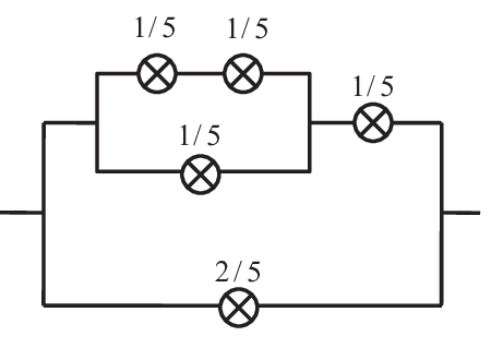
VI Conclusion

In this paper, we have studied the robustness and synthesis of stochastic switching circuits. We have shown that ssp circuits are robust against small error perturbations, while general sp circuits are not. As a result, we focused on constructing ssp circuits to synthesize or approximate probabilities. We generalized the results in [15] and proved that when $q$ is a multiple of $2$ or $3$ , all rational fractions $\frac{a}{q^{n}}$ can be realized using ssp circuits when the pswitch set $S=\{\frac{1}{q},\frac{2}{q},\dots,\frac{q-1}{q}\}$ . However, this property does not hold when $q$ is a prime number greater than $3$ . For a more general case of an arbitrary pswitch set, we proposed a greedy algorithm to construct ssp circuits. This method can approximate any desired probability with low circuit complexity and small errors.

References

[1] L. Chakrapani, P. Korkmaz, B. Akgul, and K. Palem, “Probabilistic system-on-a-chip architecture,” ACM Transactions on Design Automation of Electronic Systems, vol. 12, no. 3, pp. 1–28, 2007.
[2] M. Cook, D. Soloveichik, E. Winfree, J. Bruck, “Programmability of chemical reaction networks,” Algorithmic Bioprocesses, Natural Computing Series, pp. 543–584, 2009.
[3] P. Elias, “The efficient construction of an unbiased random sequence,” Ann. Math. Statist., vol. 43, pp. 865–870, 1972.
[4] B. Fett, J. Bruck, and M. D. Riedel, “Synthesizing stochasticity in biochemical systems,” in Proc. Annual Conference on Design Automation (DAC), pp. 640–645, 2007.
[5] A. Gill, “Synthesis of probability transformers,” Journal of the Franklin Institute, vol. 274, no. 1, pp. 1–19, 1962.
[6] A. Gill, “On a weight distribution problem, with application to the design of stochastic generators,” Journal of the ACM, vol. 10, no. 1, pp. 110–121, 1963.
[7] T. S. Han and M. Hoshi, “Interval algorithm for random number generation,” IEEE Trans. Inform. Theory, vol. 43, No. 2, pp. 599–611, 1997.
[8] P. Jeavons, D. A. Cohen, and J. Shawe-Taylor, “Generating binary sequences for stochastic computing,” IEEE Trans. Inform. Theory, vol. 40, no. 3, pp. 716–720, 1994.
[9] D. E. Knuth and A. Yao, “The complexity of nonuniform random number generation,” Algorithms and Complexity: New Directions and Recent Results, pp. 357–428, 1976.
[10] P. A. MacMahon, “The combinations of resistances,” The Electrician, 28:601–602, 1892. (Reprinted in: Discr. Appl. Math., 54:225–228, 1994.).
[11] W. Qian, M. D. Riedel, H. Zhou, and J. Bruck, “Transforming probabilities with combinational logic,” IEEE Trans. on Computer-Aided Design of Integrated Circuits and Systems, vol. 30, pp. 1279–1292, 2011.
[12] C. E. Shannon. “A symbolic analysis of relay and switching circuits,” Trans. AIEE, 57:713–723, 1938.
[13] D. Soloveichik, G. Seelig, and E. Winfree, “DNA as a universal substrate for chemical kinetics,” PNAS 107, pp. 5393–5398, 2010.
[14] J. von Neumann, “Various techniques used in connection with random digits,” Appl. Math. Ser., Notes by G.E. Forstyle, Nat. Bur. Stand., vol. 12, pp. 36–38, 1951.
[15] D. Wilhelm and J. Bruck, “Stochastic switching circuit synthesis,” in Proc. IEEE International Symposium on Information Theory (ISIT), pp. 1388–1392, 2008.

The Synthesis and Analysis of Stochastic Switching Circuits

Abstract

Index Terms:

I Introduction

II Related Works and Preliminaries

Theorem 1 (Duality Theorem [15]).

III Robustness

III-A Robustness of ssp Circuits

Theorem 2 (Robustness of ssp circuits).

Proof.

III-B Robustness of sp Circuits

Theorem 3 (Lower bound for sp circuits).

Proof.

Theorem 4 (Upper bound for sp circuits).

Proof.

III-C Robustness of Non-sp Circuits

Theorem 5 (Upper bound for general circuits).

Proof.

IV Expressibility

IV-A Backward Algorithms

IV-B Multiples of 22 or 33

Algorithm 1 (Backward algorithm to realize p1=aqnp_{1}=\frac{a}{q^{n}} with 0<a<qn0<a<q^{n} and pswitch set S={1q,2q,…,q−1q}S=\{\frac{1}{q},\frac{2}{q},\dots,\frac{q-1}{q}\}).

Theorem 6.

Proof.

Theorem 7 (Upper bound of circuit size when qq is even).

Proof.

Theorem 8 (Upper bound of circuit size when qq is odd and a multiple of 33).

Theorem 9 (Upper bound of circuit size when qq is a multiple of 66).

IV-C Prime Number Larger Than 33

Lemma 10.

Proof.

Theorem 11 (When qq is a prime number larger than 33).

V Probability Approximation

V-A Greedy Algorithm

Algorithm 2 (Greedy algorithm with step-length mm).

Lemma 12.

Proof.

V-B Approximation Error when |S|=1|S|=1

Theorem 13 (Approximation error when |S|=1|S|=1).

Proof.

V-C Approximation Error when |S|>1|S|>1

Theorem 14 (Approximation error for m=1m=1).

Proof.

Theorem 15 (Approximation error for m=2m=2).

Proof.

Theorem 16.

Proof.

VI Conclusion

References

IV-B Multiples of $2$ or $3$

Algorithm 1 (Backward algorithm to realize $p_{1}=\frac{a}{q^{n}}$ with $0<a<q^{n}$ and pswitch set $S=\{\frac{1}{q},\frac{2}{q},\dots,\frac{q-1}{q}\}$ ).

Theorem 7 (Upper bound of circuit size when $q$ is even).

Theorem 8 (Upper bound of circuit size when $q$ is odd and a multiple of $3$ ).

Theorem 9 (Upper bound of circuit size when $q$ is a multiple of $6$ ).

IV-C Prime Number Larger Than $3$

Theorem 11 (When $q$ is a prime number larger than $3$ ).

Algorithm 2 (Greedy algorithm with step-length $m$ ).

V-B Approximation Error when $|S|=1$

Theorem 13 (Approximation error when $|S|=1$ ).

V-C Approximation Error when $|S|>1$

Theorem 14 (Approximation error for $m=1$ ).

Theorem 15 (Approximation error for $m=2$ ).