Universal microstructure and mechanical stability of jammed packings
Abstract
Jammed packings’ mechanical properties depend sensitively on their detailed local structure. Here we provide a complete characterization of the pair correlation close to contact and of the force distribution of jammed frictionless spheres. In particular we discover a set of new scaling relations that connect the behavior of particles bearing small forces and those bearing no force but that are almost in contact. By performing systematic investigations for spatial dimensions =3–10, in a wide density range and using different preparation protocols, we show that these scalings are indeed universal. We therefore establish clear milestones for the emergence of a complete microscopic theory of jamming. This description is also crucial for high-precision force experiments in granular systems.
pacs
64.70.Q-,05.20.-y,61.20.-p,81.05.KfIntroduction –
The jamming phenomenon is ubiquitous – candies [1], coal [2], and colloids [3] all can jam, but its microscopic universality remains debated, even for the most ideal of systems. Like any other phase transition, the jamming transition can be approached from the unjammed phase, e.g. by compressing hard spheres (HS) [4], or from the jammed phase, e.g. by minimizing the energy of soft spheres (SS) [5]. Yet these two complementary approaches have mostly been developed independently from each other (see [6] for HS and [7, 8] for SS). Unlike standard phase transitions, however, the jamming transition is a non-equilibrium phenomenon that happens deep inside the glass phase [9, 10], and therefore different protocols generate different packings, which may result to conflicting observations. Indeed, all agree that marginally stable packings of frictionless spheres average force-bearing contacts per particle [8], but jammed packings’ density [11, 12, 6, 13, 14], parts of their microstructure [15, 16, 6], as well as their given name [17, 6] are contentious. Although the jamming “j” point was proposed to be unique in the thermodynamic limit [5, 18], there is a growing consensus that jamming occurs over a range of “j” points [17, 6, 9, 14, 13, 7]. Yet various physical origins have been attributed to the jamming density variation, including structural correlations in the initial configuration [7], and the presence of small crystalline regions only detectable by subtle order metrics whose minimization should result in a single “maximally random jammed” state [17, 6]. Others have proposed the intrinsic existence of a range of densities over which packings with an identically disordered structure could be found [9, 14, 13]. A power-law growth of the number of almost-touching particles near jamming has also been identified numerically, but different exponents have been found for HS [4] and SS [15]. If there is microscopic universality, it has yet to fully emerge.
In this letter we bring a different point of view to the problem by systematically investigating how the jamming limit is approached from both sides of the transition and by varying the dimensionality of space from =3 to 10. This approach allows us to obtain a series of important results. (1) Increasing suppresses crystallization [19, 20] and the “spurious” contribution of “rattlers”. We can thus show that random jammed packings of monodisperse spheres with identical near-contact structural properties can be obtained over a range of densities (thus confirming results in =3, 4 [17, 4, 19, 14, 21]), and that this range broadens with increasing . (2) We confirm an earlier suggestion that two exponents and , corresponding to different physical regimes, control the mechanical stability of jammed packings [22]. The first describes the “quasi-contact” regime in which particles are separated by very small gaps , whose number scales as for small ; the second describes the tail of the “contact” regime, where the number of particles bearing a small force scales as . (3) We also provide a complete characterization of the microstructure of jammed packings. We show that matching the two above regimes provides scaling relations between the exponents and non-trivial scaling functions. We thus conclude that the mechanical stability of jammed packings is related to their very complex contact microstructure. (4) We find these results to be universal in the sense that they are robust to changes in preparation protocol, packing density, and, in particular, spatial dimension.
The observation that jammed packings’ properties are independent of suggests that a mean-field theory should be able to capture the jamming phenomenology [23, 24]. One such treatment, the Gaussian replica theory (G-RT) [13, 10], unifies the description of the glass transition and of jamming by exploiting an analogy with discrete random optimization problems [25, 9]. In this treatment, the HS and SS approaches to jamming are unified under the assumption that jammed states are the infinite pressure (for HS) or zero temperature (for SS) limit of long-lived metastable glassy states [13, 10]. The theory predicts a growing jamming density range with [13], the existence of scaling relations for energy and pressure relating the two sides of the jamming transition [10], and makes structural scaling predictions that are remarkably satisfied at short distances [13, 10]. Yet we show here that (5) G-RT completely fails to describe the structural regime that controls jammed packings’ mechanical stability. Our results (1)-(5) will thus guide both theory and experiments (through high-precision force measurements [26]) towards a better understanding of the jamming transition.
Packing Generation –
We consider a system of identical spherical particles of diameter in a fixed volume , under periodic boundary conditions. The packing fraction , where is the volume of a -dimensional sphere of radius , measures the fraction of space occupied by particles. Jammed packings are prepared using two different numerical protocols (see Appendix for details and reduced units definitions). (i) Approaching jamming from densities below it by Lubachevsky-Stillinger (LS) compressions of HS undergoing Newtonian dynamics while grows at a fixed rate = [4]. The compression, which is tuned to prevent crystallization [20, 27], stops when particles are very near contact, defining the packing fraction at which the HS reduced pressure becomes infinite. (ii) Approaching jamming from densities above or below it by minimizing the energy of a random configuration of harmonic SS. Initial bounds and that bracket jamming are evolved iteratively by choosing an intermediate value and minimizing the energy of the current configuration at (procedure from above) or at (procedure from below). The final jammed configurations at the onset of have from above and from below. From above, the energy vanishes with and the static pressure , where is the distance from jamming [5].

We find the initial to have no measurable effect on . We formally define , but any reasonable results in the same final density. By contrast, strongly depends on (Fig. 1), but is also independent of . We therefore define . A practical way of constructing both and is to run the energy minimization (respectively from below and from above) starting from and large enough to saturate to its maximum. Intermediate packing fractions can then be obtained by reducing (Fig. 1). By varying in protocol (ii) we can thus construct packings over a density interval that roughly corresponds in protocol (i) to with and (larger generate mechanically unstable packings). The resulting density range is remarkably found to grow steadily from about in to nearly in (Fig. 1). We therefore confirm the similar observation made for binary mixtures [14], where the limited available density range and the subtle crystal order had left some room for debate [6]. Note that this range is achieved by only implementing procedures that compact liquid configurations. Ref. [21] has shown that enlarging the space of procedures enlarges the range of jammed packings, but the resulting packings likely have a different microstructure.
The similarity between the jamming density results of the two protocols suggests an underlying physical connection between them. G-RT indeed predicts that packings exist over a finite packing fraction range, whose upper limit is the “glass close packing” [13]. By analogy with random combinatorial optimization problems [25], the densest packing at is conjectured to require a time to generate, the exponent being possibly , based on a nucleation analysis. The maximal density that can be reached by the protocols above, which both run in polynomial time in , should therefore be strictly smaller than . Figure 1 shows it to be the case for all , in agreement with G-RT.


Scaling functions –
To determine the universal structure of disordered jammed structures, we consider the pair correlation function , which is the only relevant structural correlation in high fluids [28]. For numerical convenience, we compute the cumulative structure function
| (1) |
where is the surface of a dimensional sphere of unit radius. The function thus provides the average number of neighbors within of a given particle. Rattlers are first excluded from the analysis (Appendix), but we come back to this point below.

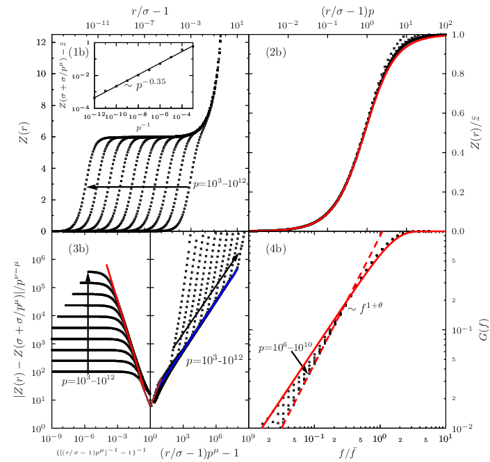
For both protocols, jumps from 0 to a plateau at on a scale proportional to the distance to jamming , where is the isostatic average number of contacts plus a correction (Fig. 2). For HS, we find =0.36(2), while =0.53(3) for SS (Fig. 3) [5]. The approach to the isostatic plateau is characterized by a long power-law tail with exponents =0.28(3) for HS and =0.42(2) for SS, but the exponent is independent of for a given model. The plateau is extended by a second power-law regime that corresponds to particles in “quasi-contact”, carrying no force at jamming. We find that in this regime the scaling is the same for both protocols, growing as with a universal exponent until it reaches the trivial large regime. Interestingly, the two power-law regimes can be matched by a scaling function , which defines an additional intermediate regime. This intermediate regime shrinks to a point at jamming, but smoothly crosses over from one power-law regime to the other at finite . Consistency therefore sets clear scaling requirements for the different regimes (see Appendix for scaling analysis) as detailed in Fig. 2, and verified in Fig. 3.
Force distribution and mechanical stability –
The consequences of these universal scaling relations on mechanical properties can be gleaned from the probability distribution of inter-particle forces . Here again, we consider the cumulative distribution rather than the pair force distribution , for numerical convenience.
For HS approaching jamming, the average force . In the contact regime the force and distance distributions are also related through a Laplace transform (Appendix) [4]. The low-force distribution is thus consistent with and . For SS approaching jamming from above, the pair potential sets the relation between the force and the pair distributions [29] (Appendix). Here again, the low-force tail is consistent with . For both protocols, however, the regime intermediate between contacts and quasi-contacts results in deviations from this power-law decay at very weak forces away from jamming.
The large force regime has been thoroughly studied [29, 5, 18, 30, 4, 31, 32], but the weak force distribution is much less well characterized. Yet it has been proposed by Wyart [22] that is required for mechanical stability. Both the SS values (, ) and the HS ones (, ), however, indicate a slight violation of this condition. A generalized stability condition of the form [22] is consistent with our findings for , but a direct test of this extended relation is beyond the scope of the current analysis.
Rattlers –
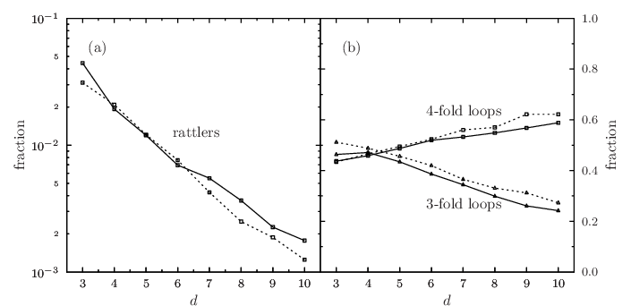
Rattlers, i.e., particles with no mechanical contacts, must be considered before concluding that the dimensional and protocol robustness of these results strongly support a universal microscopic description of jamming. Because their fraction rapidly decreases with increasing (Appendix) [19], and their structural contribution is clearly distinct from that of the other particles when , it is reasonable to remove them from the analysis. Rattlers indeed play essentially no role in the scaling regimes in high , while in low , their inclusion introduces noise in and that obscures the scaling relations, which may explain why was obtained in Ref. [15]. Removing the rattlers reveals the robust relationship between microstructure and mechanical properties, in support of jamming having a critical dimension [24].
Comparison with microscopic theory –
G-RT, the only available first-principle theory of jammed packings, provides predictions for the contact regime scaling function [13, 10] (Appendix). We find the form of to be extremely accurate when is of order 1, but G-RT fails to capture the ensuing power-law regimes (Fig. 3). G-RT indeed predicts an exponent for both protocols, and completely misses the power-law divergence related to , predicting . A similar deviation is observed at weak forces. We attribute these discrepancies to the Gaussian assumption for the cage form of G-RT, which has recently been found to be erroneous in dense disordered fluids [33, 34]. This non-Gaussian structure also naturally suggests a microscopic explanation for the breakdown of the normal-mode decomposition of jammed states [35, 36]. Including a non-Gaussian cage to RT ought to provide a better mean-field understanding of the jamming phenomenology.
Conclusions –
Our results show that the jamming terminology controversy should be resolved by replacing the j-point [5] with the j-line [9, 13], and by distinguishing a range of maximally random jammed packings from their partially crystallized counterparts [17, 6, 21]. They also reveal that the contacts’ complex microstructure in jammed packings is characterized by universal, well-defined scaling regimes and by their corresponding scaling functions. We give precise numerical predictions for the scaling exponents, and show that the scaling functions are related to the force probability distribution. These specific predictions can be tested in soft matter and granular experiments. A preliminary investigation indeed examined the scaling of the peak of the pair correlation function [3], but our comprehensive predictions can help experimentalists access the full scaling of and . This feat should be possible once a force resolution of is experimentally achieved [26].
Finally, it is worth noting that the present study was limited to zero temperature in the sense that no thermal motion is allowed in SS and that for HS the energy interaction scale is infinite compared to . At finite , the jamming transition is blurred [10], but vestiges of the scaling relations should remain visible [3]. Future work will detail how temperature and its associated anharmonicities affect the scaling relations identified here [10, 35].
Acknowledgments –
We acknowledge discussions with S. Torquato and S. Nagel. The European Research Council has provided financial support through ERC grant agreement no. 247328. P.C. acknowledges National Science Foundation support no. DMR-1055586.
References
- [1] A. Donev, I. Cisse, D. Sachs, E. Variano, F. Stillinger, R. Connelly, S. Torquato, and P. Chaikin, Science 303, 990 (2004).
- [2] D. Frenkel, physics 3, 37 (2010).
- [3] Z. Zhang, N. Xu, D. Chen, P. Yunker, A. Alsayed, K. Aptowicz, P. Habdas, A. Liu, S. Nagel, and A. Yodh, Nature 459, 230 (2009).
- [4] A. Donev, S. Torquato, and F. H. Stillinger, Phys. Rev. E 71, 011105 (2005).
- [5] C. S. O’Hern, S. A. Langer, A. J. Liu, and S. R. Nagel, Phys. Rev. Lett. 88, 075507 (2002).
- [6] S. Torquato and F. H. Stillinger, Rev. Mod. Phys. 82, 2633 (2010).
- [7] A. Liu, S. Nagel, W. Van Saarloos, and M. Wyart, in Dynamical Heterogeneities and Glasses, edited by L. Berthier, G. Biroli, J.-P. Bouchaud, L. Cipelletti, and W. van Saarloos (Oxford University Press, 2011).
- [8] M. van Hecke, J. Phys.: Condens. Matt. 22, 033101 (2010).
- [9] R. Mari, F. Krzakala, and J. Kurchan, Phys. Rev. Lett. 103, 025701 (2009).
- [10] L. Berthier, H. Jacquin, and F. Zamponi, Phys. Rev. E 84, 051103 (2011).
- [11] C. Song, P. Wang, and H. Makse, Nature 453, 629 (2008).
- [12] R. D. Kamien and A. J. Liu, Phys. Rev. Lett. 99, 155501 (2007).
- [13] G. Parisi and F. Zamponi, Rev. Mod. Phys. 82, 789 (2010).
- [14] P. Chaudhuri, L. Berthier, and S. Sastry, Phys. Rev. Lett. 104, 165701 (2010).
- [15] L. E. Silbert, A. J. Liu, and S. R. Nagel, Phys. Rev. E 73, 041304 (2006).
- [16] M. Clusel, E. I. Corwin, A. O. N. Siemens, and J. Brujic, Nature 460, 611 (2009).
- [17] S. Torquato, T. M. Truskett, and P. G. Debenedetti, Phys. Rev. Lett. 84, 2064 (2000).
- [18] C. S. O’Hern, L. E. Silbert, A. J. Liu, and S. R. Nagel, Phys. Rev. E 68, 011306 (2003).
- [19] M. Skoge, A. Donev, F. H. Stillinger, and S. Torquato, Phys. Rev. E 74, 041127 (2006).
- [20] J. A. van Meel, B. Charbonneau, A. Fortini, and P. Charbonneau, Phys. Rev. E 80, 061110 (2009).
- [21] Y. Jiao, F. Stillinger, and S. Torquato, J. Appl. Phys. 109, 013508 (2011).
- [22] M. Wyart, “Stability at random close packing,” (2012), arXiv:1202.0259 .
- [23] M. Wyart, Europhys. Lett. 89, 64001 (2010).
- [24] C. P. Goodrich, A. J. Liu, and S. R. Nagel, Phys. Rev. Lett. 109, 095704 (2012).
- [25] F. Krzakala and J. Kurchan, Phys. Rev. E 76, 021122 (2007).
- [26] T. S. Majmudar, M. Sperl, S. Luding, and R. P. Behringer, Phys. Rev. Lett. 98, 058001 (2007).
- [27] P. Charbonneau, A. Ikeda, G. Parisi, and F. Zamponi, Phys. Rev. Lett. 107, 185702 (2011).
- [28] H. L. Frisch and J. K. Percus, Phys. Rev. E 60, 2942 (1999).
- [29] C. S. O’Hern, S. A. Langer, A. J. Liu, and S. R. Nagel, Phys. Rev. Lett. 86, 111 (2001).
- [30] E. Corwin, H. Jaeger, and S. Nagel, Nature 435, 1075 (2005).
- [31] A. R. T. van Eerd, W. G. Ellenbroek, M. van Hecke, J. H. Snoeijer, and T. J. H. Vlugt, Phys. Rev. E 75, 060302 (2007).
- [32] F. Radjai, S. Roux, and J. Moreau, Chaos 9, 544 (1999).
- [33] F. Lechenault, R. Candelier, O. Dauchot, J.-P. Bouchaud, and G. Biroli, Soft Matter 6, 3059 (2010).
- [34] P. Charbonneau, A. Ikeda, G. Parisi, and F. Zamponi, Proc. Nat. Acad. Sci. U.S.A. 139, 13939 (2012).
- [35] C. F. Schreck, T. Bertrand, C. S. O’Hern, and M. D. Shattuck, Phys. Rev. Lett. 107, 078301 (2011).
- [36] N. Xu, V. Vitelli, A. J. Liu, and S. R. Nagel, Europhys. Lett. 90, 56001 (2010).
Appendix A Numerical simulations
Molecular dynamics simulations of HS and SS energy minimizations of = spheres in =3, =8000 in , and = in =10 are performed under periodic boundary conditions. For , the choice of a very large system is motivated by the need of reducing the statistical noise in the intermediate scaling regime for Fig. 3 of the main text. The system sizes chosen ensure that even when the system is at its densest the box edge remains larger than , which prevents a particle from ever having two direct contacts with another one. There are strong reasons to believe that although relatively small these nonetheless provide a reliable approximation of bulk behavior. First, with increasing the largest diagonals of the simulation box are larger than the box edge. Second, correlations of the fluid structure are expected to decrease very quickly with increasing [28, 19], and correspondingly finite-size effects are reduced. The validity of these rationalizations, which are consistent with the decorrelation property of high sphere packings [6], have been satisfactorily tested in in Ref. [27].
A.1 Hard Sphere LS Compressions
Event-driven HS simulations are performed at thermostated inverse temperature for spheres of mass , starting from random configurations in the limit . Time has units of [19, 27], but all dimensional quantities are expressed in units such that and . The reduced pressure , with for pressure , diverges at the jamming packing fraction as with [4]. Crystallization in is strongly suppressed, so access to deeply supersaturated starting configurations can be attained via the slow growth rate [19, 20]. In , where the crystallization of monodisperse hard spheres is relatively rapid for moderately high packing fractions, is employed up to , but the slow compression rate is used afterwards. The force between particles in high configurations is measured from the rate of momentum exchange between pairs of particles in simulations with . These measurements are made over at least collisions per particle.
A.2 Soft Sphere Energy Minimizations
The harmonic SS energy is with and . Units are chosen such that . We start from random sphere configurations and use and that bracket the jamming point, i.e., , . Jamming is identified as the onset of non-zero energy, iteratively determined using a bisection method. At each iteration, an intermediate value is chosen, and the energy at is minimized via conjugate-gradient (CG) minimization starting from either (from above) or (from below). The configuration obtained after minimization then substitutes if , or if . The procedure stops when either of two conditions is satisfied: the energy per particle falls below , corresponding to typical overlaps of the order of ; or the change in from one minimization step to the next is less than the bound set by double precision arithmetic, i.e., . The final value of defines the final packing fraction in the procedure from below and that of in the procedure from above.
A.3 Rattler Analysis
The rattlers are self-consistently determined by identifying the number of particles with fewer than neighbors within a distance cutoff for the smallest obtained by a given approach to jamming. In HS, a cutoff of is used, which roughly corresponds to a cutoff of for SS, where the scaling variable . This cutoff slightly overestimates the number of rattlers at jamming, but the rapid diminution of the fraction of rattlers with (Supplementary Fig. 7) guarantees the robustness of the results.
A.4 Extraction of the jamming density

Following [27], for each compression run at fixed we perform a linear fit of the line vs with . The point where the linear fit vanishes, indicating infinite pressure, defines for this given run. Next, for a fixed dimension, we fit to extrapolate the jamming density at .
For the energy minimization protocol, when approaching jamming from above, the jamming density can be obtained by accurately fitting the energy data with (inset in Supplementary Fig. 4). We focus in particular on minimization runs performed with initial and , which in practice correspond to taking the largest at which no variation of is detected. The associated prefactor can then be compared with the prediction from G-RT. A good agreement is obtained when the correction discussed in [10, Section VI.B] is taken into account (Supplementary Fig. 4).
Note that and are quite close to each other. They indicate the best packing density that can be reached using our two different compression protocols. Note that according to G-RT both should be smaller than the maximal packing density of glassy states, called glass close packing . According to the theory, it is very unlikely that packings at can be produced in polynomial time, hence it is expected that both and are smaller than .
Appendix B Scaling functions
B.1 Structure Scaling Analysis
When approaching jamming with protocol (i), for , and for , parametrizes the scaling function for . A first scaling regime sees grow from 0 to the average number of “contacts” as
| (2) |
with when for a constant [4]. Force-bearing contacts are only observed at jamming proper, but their signature develops asymptotically. A second regime for finite has
| (3) |
where is a constant. At jamming, these nearly touching “quasi-contacts” carry no force. For large , a trivial regime develops independently of (Sec. B.3). Matching the first two scaling regimes implies the existence of an additional intermediate regime for
| (4) |
with and . Consistency then requires that and with scaling relations and .
When approaching jamming with protocol (ii) from above, the remaining overlaps provide a scaling variable [10]. In spite of the very different preparation protocol, similar structural regimes are identified. In the contact regime, grows from 0 to by a universal scaling function
| (5) |
with when for a constant . For , here again
| (6) |
hence the two regimes must be matched by an intermediate scaling function for
| (7) |
with and . Consistency here requires that and with and .
In both cases, the exponents and are determined by collapsing the numerical results using this scaling form, which was repeated for different systems. This constraint leaves a relatively small uncertainty on the final value, which provides the error bar.

B.2 Force Scaling Analysis
When HS approach jamming, the cumulative force distribution approaches a scaling function defined by . The relation between the scaling functions and suggested in Ref. [4]
| (8) |
is verified in Supplementary Fig. 5. It follows that if for , then for , which is here observed for all (Supplementary Fig. 5). When SS approach jamming from above, the interaction potential gives for and zero otherwise, so . In the jamming limit , and therefore , as in the previous case. This behavior is here observed in all (Supplementary Fig. 5).
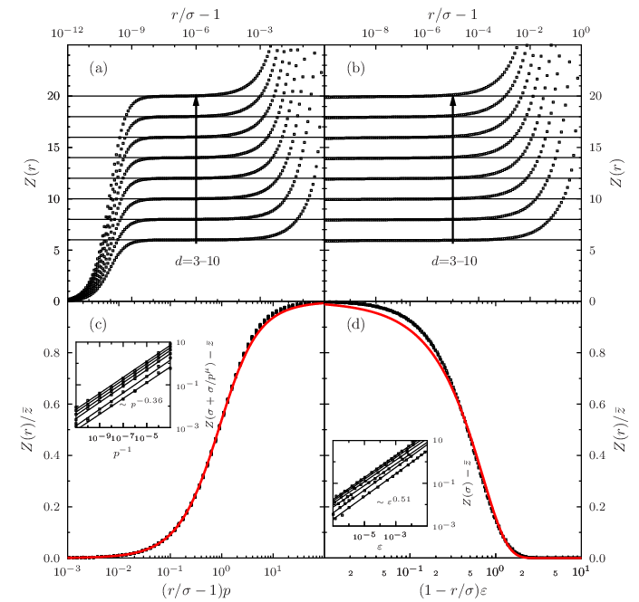

B.3 High Structure
In the contact regime , G-RT predicts that scaling functions should describe the growth of from 0 to the isostatic value, as given in Eqs. (20) and (27). Both results are tested in Supplementary Fig. 6 for =3–10. The collapse is remarkably good for all . The agreement with the G-RT scaling form is also remarkable for small , but start to deviate from the theoretical prediction when approaches the isostatic plateau. The type of deviation is different from each protocol, but is similar from one dimension to the next for a given protocol. For larger in the near-contact region, the two protocols robustly produce the same power-law growth, with (Supplementary Fig. 6), which is not predicted by G-RT. Because the number of rattlers vanishes with dimension neither of these phenomena can be ascribed to their presence. But because G-RT predictions rely on the individual cages to be Gaussian, which presumably they are not [14, 33, 34], it is natural to ascribe the discrepancy to the breakdown of that assumption.
At very large distances, the pair correlation function of any disordered systems trivially has , which corresponds to . Unsurprisingly this scaling form captures well the behavior of for both protocols and all at large , but the range of validity also extends with (Supplementary Fig. 6). In order to quantify this effect, we fit the curves of for using the form
| (9) |
When grows, the region where the second term is much bigger than the first is
| (10) |
hence . The fitted values of indicate that the crossover point indeed decreases slowly with .
Appendix C Replica theory calculations
The predictions of G-RT presented in this work are based on earlier results [13, 10]. Yet because the calculations in Ref. [10] have only been explicitly carried out for , and because different observables are considered, additional results are here presented. They are reported in this section and incidentally provide a somehow simplified derivation of the results of Ref. [10]. Nonetheless, reading this section requires a detailed knowledge of Refs [13, 10], so the reader who is not interested in the theoretical details can safely skip it. Note that as in the main text, this section uses reduced units and .
C.1 General expressions
The approximation scheme used is based on [10, Eq. (22) and (23)], which give the replicated free entropy separated between the harmonic and the liquid contributions
| (11) |
for replicas at temperature , in a Gaussian cage of variance . The function is defined in [10, just after Eq. (16)] where is a normalized and centered Gaussian of variance , and is the HS cavity function. Introducing bipolar coordinates, as in [13, Appendix C.2.a], we obtain the generalization of [13, Eq. (C16)] to the soft sphere potential
| (12) |
The above equations (11) and (12) are the starting point of all the needed replica calculations for our analysis, and because we focus on the “jamming limit” of these equations, we take with and held constant [10]. In Ref. [10] this limit was taken using a simplified form of Eq. (12) for , but we here generalize the calculation to arbitrary . The crucial observation [13, Eq. (C21)] is that when , . In the jamming limit the term in the second line of Eq. (12) therefore disappears, because while and are of order 1. The remaining integral can then be evaluated via the saddle point approximation, because both and diverge. Consider first the case . Assuming that the saddle point , one has to maximize the function which consistently maximizes . Consider next the case . Assuming that in this case , we have and we thus consistently find . Replacing these expressions for in Eq. (12) and taking the jamming limit we obtain
| (13) |
and Eq. (11) reduces to
| (14) |
which replaces [10, Eqs. (D3) and (D4)].
The approach to jamming from above is described by the small limit [10, Appendix D.2]. In this limit we can consider the SS Mayer function as a small perturbation of the HS one and use standard liquid perturbation theory to write
| (15) |
Plugging this result in Eq. (14) we then get
| (16) |
Note en passant that the cancellation of the second term in Eq. (15) with a corresponding term in is not surprising, as stated in [10, Appendix D.2], but has a deep physical interpretation. Indeed, Eq. (14) shows that the “bare” SS potential is modified around jamming by the presence of additional replicas (with ) that “renormalize” it to , as obtained in Eq. (13). The crucial point is that the latter potential does not have a singularity when , ensuring a smooth crossover and appropriate scalings around jamming.
C.2 The energy prefactor
Starting from Eq. (16) and repeating the calculations of Ref. [10, Appendix D.2], we finally obtain the quadratic scaling of the energy as a function of when approaching jamming from above. The general expression for the prefactor is then easily obtained. A further simplification is obtained by assuming that is small at the jamming point, and developing the resulting expressions in powers of [13]. Doing so and optimizing over and , one finally obtains
| (17) |
The second line recovers the result of Ref. [13, Eq. (77)]. The glass close packing point [13], which is defined by the complexity , is reported in Fig. 1. The first line shows that is indeed very small, being in and decreasing with dimension. Linearizing the last line around and using that vanishes linearly, one obtains the quadratic scaling of the energy and its prefactor [10]. G-RT results in Supplementary Fig. 4 have been obtained from this procedure, using the Carnahan-Starling equation of state in dimensions for the HS liquid [13, Eq. (82)].
A last remark on the energy prefactor is in order. G-RT results in a discrepancy between the pressure computed from thermodynamics and that computed from the structural (see Refs. [13, Eq. (89)] and [10, Section VII.B]). This difference might have its origin in the fact that only two-body effective replica interactions are kept in this treatment. Indeed in the limit , where this approximation should be exact, the discrepancy disappears. It has also been observed in Ref. [10, Section VI.B] that a much better agreement between theory and numerical data is obtained if the distance from jamming is corrected to account for this discrepancy. The correction factor obtained from the theory corresponds to the factor needed to impose the equality in [13, Eq. (89)], so rescaling is equivalent to rescaling . The rescaled predictions are also reported in Supplementary Fig. 4.
C.3 Scaling functions
To complete the analysis we compute the scaling functions predicted by G-RT. Consider first the HS case, approaching jamming from below. The contact peak of on approaching jamming is given by [13, Eq. (90)]
| (18) |
where . The validity of the thermodynamic relation is here assumed. As we discussed above, this relation is violated by the theory, but the correction is here unimportant. If one does not want to use this relation, it is sufficient to replace , but in the end this substitution does not affect the prediction for the scaling function.
Integrating Eq. (18) using Eq. (1) we get, after changing the variable to
| (19) |
We notice now that and . The integration is therefore over an interval of order 1. The first term in the integrand can be neglected because for of order 1, so this term goes to 1 when . Finally we obtain in the contact region
| (20) |
where . This prediction is tested in Fig. 3 of the main text and in Supplementary Fig. 6.
Next consider the SS case approaching jamming from above, working in the jamming limit. with and . In this case the calculation starts from [10, Eqs. (17) and (48)]. Using bipolar coordinates we can write
| (21) |
We now need to improve Eq. (13) by considering the quadratic corrections around the saddle point, which for leads to
| (22) |
Plugging Eq. (22) in Eq. (21), dropping as before the last term in square brackets in Eq. (21), and evaluating the integral via the saddle point approximation including quadratic corrections, we find for that
| (23) |
Plugging this result in Eq. (1), and assuming that we approach jamming from above, so that , we obtain for that
| (24) |
Changing variables to and using the first line of Eq. (17) gives
| (25) |
Although this result is already the desired scaling function, we can further simplify it by noting that is small to write
| (26) |
where in the last line we used the last line of Eq. (17). The resulting prediction
| (27) |
is tested in Fig. 3 of the main text and in Supplementary Fig. 6.