跳到论文正文
W Papers独立论文阅读器 arXiv:1209.0633 论文正文 计算阅读时间 · 0%
引用这篇论文根据当前论文元数据生成,正式投稿前建议核对。


License: arXiv.org perpetual non-exclusive license
arXiv:1209.0633v4 [math.ST] 26 Aug 2015

Nonparametric regression on hidden Φ\Phi-mixing variables: identifiability and consistency of a pseudo-likelihood based estimation procedure

Thierry Dumont Note: MODAL’X, Université Paris-Ouest, Nanterre, France. thierry.dumont@u-paris10.fr    Sylvain Le Corff Note: Laboratoire de Mathématiques, Université Paris-Sud and CNRS, Orsay, France. sylvain.lecorff@math.u-psud.fr
Abstract

This paper outlines a new nonparametric estimation procedure for unobserved Φ\Phi-mixing processes. It is assumed that the only information on the stationary hidden states (Xk)k≥0(X_{k})_{k\geq 0} is given by the process (Yk)k≥0(Y_{k})_{k\geq 0}, where YkY_{k} is a noisy observation of f⋆​(Xk)f_{\star}(X_{k}). The paper introduces a maximum pseudo-likelihood procedure to estimate the function f⋆f_{\star} and the distribution νb,⋆\nu_{b,\star} of (X0,…,Xb−1)(X_{0},\dots,X_{b-1}) using blocks of observations of length bb. The identifiability of the model is studied in the particular cases b=1b=1 and b=2b=2 and the consistency of the estimators of f⋆f_{\star} and of νb,⋆\nu_{b,\star} as the number of observations grows to infinity is established.

1 Introduction

The model considered in this paper consists of a bivariate stochastic process {(Xk,Yk)}k≥0\{(X_{k},Y_{k})\}_{k\geq 0} where only the sequence (Yk)k≥0(Y_{k})_{k\geq 0} is observed. These observations are given by

Yk=f⋆​(Xk)+ϵk,Y_{k}=f_{\star}(X_{k})+\epsilon_{k}\;, (1)

where f⋆f_{\star} is a function defined on a space 𝕏\mathbb{X} and taking values in ℝℓ\mathbb{R}^{\ell}. The measurement noise (ϵk)k≥0(\epsilon_{k})_{k\geq 0} is an independent and identically distributed (i.i.d.) sequence of Gaussian random vectors of ℝℓ\mathbb{R}^{\ell}. This paper proposes a new method to estimate the function f⋆f_{\star} and the distribution of the hidden states using only the observations (Yk)k≥0(Y_{k})_{k\geq 0}. Nonparametric estimation with latent random variables is a challenging task and most of the existing results in this context use additional assumptions on the sequence (Xk)k≥0(X_{k})_{k\geq 0}. For instance, in errors-in-variables models, the random variables (Xk)k≥0(X_{k})_{k\geq 0} are observed through a sequence (Zk)k≥0(Z_{k})_{k\geq 0}, i.e. Zk=Xk+ηkZ_{k}=X_{k}+\eta_{k} and Yk=f⋆​(Xk)+ϵkY_{k}=f_{\star}(X_{k})+\epsilon_{k}, where the variables (ηk)k≥0(\eta_{k})_{k\geq 0} are i.i.d with known distribution. Many solutions have been proposed to solve this problem, see [12] and [15] for a ratio of deconvolution kernel estimators, [17] for B-splines estimators and [5] for a procedure based on the minimization of a penalized contrast. In the case where the hidden state is a Markov chain, [20, 19] considered the following observation model Yk=Xk+ϵkY_{k}=X_{k}+\epsilon_{k}, where the random variables {ϵk}k≥0\{\epsilon_{k}\}_{k\geq 0} are i.i.d. with known distribution. [20] (resp. [19]) proposed an estimator of the transition density (resp. the stationary density and the transition density) of the Markov chain (Xk)k≥0(X_{k})_{k\geq 0} based on the minimization of a penalized L2\mathrm{L}_{2} contrast.

Recently, [10] used the model (1) for indoor simultaneous localization and mapping based on WiFi signals. In this framework, the process (Xk)k≥0(X_{k})_{k\geq 0} is the position of a mobile device evolving in a building and it is assumed to be a Markov chain with transition density depending only on the distance between two consecutive states. YkY_{k} denotes the signal strengths measured by the device at time step kk. Only (Yk)k≥0(Y_{k})_{k\geq 0} is observed and inference on the hidden positions (Xk)k≥0(X_{k})_{k\geq 0} (localization) requires an efficient estimation of f⋆f_{\star} (mapping).

In this paper, the random process (Xk)k≥0(X_{k})_{k\geq 0} is assumed to be Φ\Phi-mixing and stationary which encompasses the i.i.d. case and the hidden Markov model setting of [10]. We propose a new approach to estimate the function f⋆f_{\star} and the distribution νb,⋆\nu_{b,\star} of the hidden states (X0,…,Xb−1)(X_{0},\dots,X_{b-1}) for a given bb using only the observations (Yk)k≥0(Y_{k})_{k\geq 0}. The identifiability of the model is studied and we show that for some particular cases, f⋆f_{\star} may be recovered up to an isometric transformation of 𝕏\mathbb{X}. The observations are decomposed into non-overlapping blocks (Yk​b,…,Y(k+1)​b−1)(Y_{kb},\dots,Y_{(k+1)b-1}) to define a pseudo likelihood function. The estimator (f^n,ν^n)(\widehat{f}_{n},\widehat{\nu}_{n}) of (f⋆,νb,⋆)(f_{\star},\nu_{b,\star}) is defined as a maximizer of a penalized version of the pseudo-likelihood of the observations (Y0,…,Yn​b−1)(Y_{0},\dots,Y_{nb-1}) over a class of functions ℱ\mathcal{F} and a class of densities 𝒟b\mathcal{D}_{b} on 𝕏b\mathbb{X}^{b}. These estimators of f⋆f_{\star} and νb,⋆\nu_{b,\star} may then be used to define an estimator p^n\widehat{p}_{n} of the density of the distribution of (Y0,…,Yb−1)(Y_{0},\dots,Y_{b-1}). It is proved in Section 3 that the Hellinger distance between p^n\widehat{p}_{n} and the true distribution of a block of observations vanishes as the number of observations grows to infinity. This result is established using few assumptions on the model: the penalization function needs only to be lower bounded by a power of the supremum norm and no topological restrictions are made on 𝕏\mathbb{X}. Under compacity assumptions on ℱ\mathcal{F} and 𝒟b\mathcal{D}_{b} the consistency of (f^n,ν^n)(\widehat{f}_{n},\widehat{\nu}_{n}) is derived although the rate of convergence of (f^n,ν^n)(\widehat{f}_{n},\widehat{\nu}_{n}) remains an open problem and seems to be very challenging.

In Section 4, we discuss the identifiability issues raised by the model (1). When b=1b=1, the identifiability is studied in the particular case where 𝕏\mathbb{X} is a subset of ℝm\mathbb{R}^{m} for some m>0m>0, f⋆f_{\star} is a 𝒞1\mathcal{C}^{1} diffeomorphism and ℱ\mathcal{F} is a subset of continuously differentiable functions on 𝕏\mathbb{X}. We establish that if X~0\tilde{X}_{0} has a distribution with probability density ν\nu and if f~∈ℱ\tilde{f}\in\mathcal{F} is such that f~​(X~0)\tilde{f}(\tilde{X}_{0}) and f⋆​(X0)f_{\star}(X_{0}) have the same distribution then f~=f⋆∘ϕ\tilde{f}=f_{\star}\circ\phi and ν=|Jϕ|⋅ν1,⋆∘ϕ\nu=|J_{\phi}|\cdot\nu_{1,\star}\circ\phi where ϕ:𝕏→𝕏\phi:\mathbb{X}\to\mathbb{X} is a bijective function (|Jϕ||J_{\phi}| denotes the determinant of the Jacobian matrix of ϕ\phi). This result only requires regularity assumptions on the unknown function f⋆f_{\star} and not on the candidate function f~\tilde{f}, which in particular is not assumed to be one-to-one. This implies that the inference task may be performed within a larger class of functions. A similar result is obtained when b=2b=2 to establish that the model is identifiable up to an isometric transformation of 𝕏\mathbb{X} in the context of [10].

The consistency and identifiability results are applied in Section 5 when ℱ\mathcal{F} is assumed to be a Sobolev class of functions. In this setting, the supremum norm in ℱ\mathcal{F} may be controlled by the penalty term to ensure that p^n\widehat{p}_{n} is consistent. Moreover, this framework satisfies the compacity assumption needed in Section 3 to derive the consistency of (f^n,ν^n)(\widehat{f}_{n},\widehat{\nu}_{n}). Section 6 provides numerical experiments to illustrate our estimation approach and the identifiability results of Section 4. Proofs and technical results are postponed to Section 7 and to the appendices.

2 Model and definitions

Let (Ω,ℰ,ℙ)(\Omega,\mathcal{E},\mathbb{P}) be a probability space and (𝕏,𝒳)(\mathbb{X},\mathcal{X}) be a general state-space endowed with a measure μ\mu. Let (Xk)k≥0(X_{k})_{k\geq 0} be a stationary process defined on Ω\Omega and taking values in 𝕏\mathbb{X}. This process is only partially observed through the sequence (Yk)k≥0(Y_{k})_{k\geq 0} which takes values in ℝℓ\mathbb{R}^{\ell}, ℓ≥1\ell\geq 1. In the sequel, for any 0≤k≤k′0\leq k\leq k^{\prime}, the sequence (xk,…,xk′)(x_{k},\dots,x_{k}^{\prime}) is written xk:k′x_{k:k^{\prime}}. The observations (Yk)k≥0(Y_{k})_{k\geq 0} are given by (1) where f⋆:𝕏→ℝℓf_{\star}:\mathbb{X}\rightarrow\mathbb{R}^{\ell} is a measurable function and the random variables (ϵk)k≥0(\epsilon_{k})_{k\geq 0} are i.i.d. with density φ\varphi with respect to the Lebesgue measure λ\lambda of ℝℓ\mathbb{R}^{\ell}, given, for any z1:ℓ∈ℝℓz_{1:\ell}\in\mathbb{R}^{\ell}, by:

φ(z1:ℓ)=def(2π)−ℓ/2exp(−12∑j=1ℓzj2).\varphi(z_{1:\ell})\stackrel{{\scriptstyle\mathrm{def}}}{{=}}\left(2\pi\right)^{-\ell/2}\exp\left(-\frac{1}{2}\sum_{j=1}^{\ell}z_{j}^{2}\right)\;. (2)

In this paper, ϵ0\epsilon_{0} is assumed to be distributed according to a standard normal distribution. Note that this setting is enough to deal with a known and nonsingular covariance matrix Σ\Sigma. In this case, (Yk)k≥0(Y_{k})_{k\geq 0} may be replaced by (Σ−1/2Yk)k≥0(\Sigma^{-1/2}Y_{k})_{k\geq 0} and the modified noise Σ−1/2ϵ0\Sigma^{-1/2}\epsilon_{0} is then a standard normal random vector.

This paper proposes a method to estimate the target function f⋆∈ℱf_{\star}\in\mathcal{F}, where ℱ\mathcal{F} is a set of functions from 𝕏\mathbb{X} to ℝℓ\mathbb{R}^{\ell}, and the distribution of the hidden states using only the observations (Yk)k≥0(Y_{k})_{k\geq 0}. This problem could be interpreted as a deconvolution problem where it is usual to assume that the noise distribution is known, see for instance [3, 16, 18]. Here, the density φ\varphi is assumed to be known to simplify the proof of identifiability (Section 4). This proof only needs the characteristic function of ϵ0\epsilon_{0} to be known and non zero. Note that the Gaussian assumption is only used to establish the consistency result (Theorem 3.1) which relies on an entropy control written for this particular choice of density function. A few authors have studied the deconvolution problem with unknown noise distribution. In [4], the estimation of the density of XX in the model Y=X+ϵY=X+\epsilon is performed without knowing the distribution ϵ\epsilon and under mild assumptions on the smoothness of the underlying densities. However, [4] only considered real valued random variables and the estimation based on Fourier transform and bandwidth selection is hardly relevant in our model. The main difference between the model studied in this paper and classical convolution models is that the random vector f⋆​(Xk)f_{\star}(X_{k}) does not necessarily have a density with respect to the Lebesgue measure on ℝℓ\mathbb{R}^{\ell}. As discussed in Section 5 (Corollary 5.2), under some assumptions on f⋆f_{\star}, if the state-space 𝕏\mathbb{X} is a subset of ℝm\mathbb{R}^{m} with m<ℓm<\ell, f⋆​(Xk)f_{\star}(X_{k}) lies in a sub-manifold of dimension mm in ℝℓ\mathbb{R}^{\ell} which has a null Lebesgue measure and then classical deconvolution tools do not apply here.

Let bb be a positive integer. For any sequence (xk)k≥0(x_{k})_{k\geq 0}, define 𝐱k=def(xk​b,…,x(k+1)​b−1)\mathbf{x}_{k}\stackrel{{\scriptstyle\mathrm{def}}}{{=}}(x_{kb},\ldots,x_{(k+1)b-1}) and for any function f:𝕏→ℝℓf:\mathbb{X}\to\mathbb{R}^{\ell}, define 𝐟:𝕏b→ℝb​ℓ\mathbf{f}:\mathbb{X}^{b}\to\mathbb{R}^{b\ell} by

𝐱=(x0,…,xb−1)↦𝐟⁡(𝐱)=def(f⁡(x0),…,f⁡(xb−1)).\mathbf{x}=(x_{0},\ldots,x_{b-1})\mapsto\mathbf{f}(\mathbf{x})\stackrel{{\scriptstyle\mathrm{def}}}{{=}}(f(x_{0}),\ldots,f(x_{b-1}))\;.

The distribution of 𝐗0\mathbf{X}_{0} is assumed to have a density νb,⋆\nu_{b,\star} with respect to the measure μ⊗b\mu^{\otimes b} on 𝕏b\mathbb{X}^{b} which lies in a set of probability densities 𝒟b\mathcal{D}_{b}. For all f∈ℱf\in\mathcal{F} and ν∈𝒟b\nu\in\mathcal{D}_{b}, let pf,νp_{f,\nu} be defined, for all 𝐲∈ℝb​ℓ\mathbf{y}\in\mathbb{R}^{b\ell}, by

pf,ν​(𝐲)=def∫ν⁡(𝐱)​∏k=0b−1φ⁡(yk−f⁡(xk))​μ⊗b​(𝑑𝐱).p_{f,\nu}(\mathbf{y})\stackrel{{\scriptstyle\mathrm{def}}}{{=}}\int\nu(\mathbf{x})\prod_{k=0}^{b-1}\varphi(y_{k}-f(x_{k}))\mu^{\otimes b}\left(\mathrm{d}\mathbf{x}\right)\;. (3)

Note that pf⋆,νb,⋆p_{f_{\star},\nu_{b,\star}} is the probability density of 𝐘0\mathbf{Y}_{0} defined in (1): for all 𝐲∈ℝb​ℓ\mathbf{y}\in\mathbb{R}^{b\ell},

p⋆​(𝐲)=defpf⋆,νb,⋆​(𝐲)=∫νb,⋆​(𝐱)​∏k=0b−1φ⁡(yk−f⋆​(xk))​μ⊗b​(𝑑𝐱).p_{\star}(\mathbf{y})\stackrel{{\scriptstyle\mathrm{def}}}{{=}}p_{f_{\star},\nu_{b,\star}}(\mathbf{y})=\int\nu_{b,\star}(\mathbf{x})\prod_{k=0}^{b-1}\varphi(y_{k}-f_{\star}(x_{k}))\mu^{\otimes b}\left(\mathrm{d}\mathbf{x}\right)\;. (4)

The function y0:n​b−1↦∑k=0n−1lnpf,ν(𝐲k)y_{0:nb-1}\mapsto\sum_{k=0}^{n-1}\ln p_{f,\nu}\left(\mathbf{y}_{k}\right) is referred to as the pseudo log-likelihood of the observations up to time n​b−1nb-1. This paper introduces an estimation procedure based on the method of M-estimation presented in [26] and [25]. Consider a function I:ℱ→ℝ+I:\mathcal{F}\rightarrow\mathbb{R}^{+} which characterizes the complexity of functions in ℱ\mathcal{F} and let δn\delta_{n} and λn\lambda_{n} be some positive numbers. Define the following δn\delta_{n}-Maximum Pseudo-Likelihood Estimator (δn\delta_{n}-MPLE) of (f⋆,νb,⋆)(f_{\star},\nu_{b,\star}):

(f^n,ν^n)=defargmaxδnf∈ℱ,ν∈𝒟b​{∑k=0n−1ln⁡pf,ν​(𝐘k)−λn​I​(f)},\left(\widehat{f}_{n},\widehat{\nu}_{n}\right)\stackrel{{\scriptstyle\mathrm{def}}}{{=}}\underset{f\in\mathcal{F},\ \nu\in\mathcal{D}_{b}}{\mbox{argmax}^{\delta_{n}}}\left\{\sum_{k=0}^{n-1}\ln p_{f,\nu}\left(\mathbf{Y}_{k}\right)-\lambda_{n}I(f)\right\}\;, (5)

where argmaxδnf∈ℱ,ν∈𝒟b\underset{f\in\mathcal{F},\ \nu\in\mathcal{D}_{b}}{\mbox{argmax}^{\delta_{n}}} is one of the pairs (f′,ν′)(f^{\prime},\nu^{\prime}) such that

∑k=0n−1ln⁡pf′,ν′​(𝐘k)−λn​I​(f′)≥supf∈ℱ,ν∈𝒟b{∑k=0n−1ln⁡pf,ν​(𝐘k)−λn​I​(f)}−δn.\sum_{k=0}^{n-1}\ln p_{f^{\prime},\nu^{\prime}}\left(\mathbf{Y}_{k}\right)-\lambda_{n}I(f^{\prime})\geq\sup_{f\in\mathcal{F},\ \nu\in\mathcal{D}_{b}}\left\{\sum_{k=0}^{n-1}\ln p_{f,\nu}\left(\mathbf{Y}_{k}\right)-\lambda_{n}I(f)\right\}-\delta_{n}\;.

The consistency of the estimators is established using a control for empirical processes associated with mixing sequences. The Φ\Phi-mixing coefficient between two σ\sigma-fields 𝒰,𝒱⊂ℰ\mathcal{U},\mathcal{V}\subset\mathcal{E} is defined in [7] by

Φ⁡(𝒰,𝒱)=defsupU∈𝒰,V∈𝒱,ℙ⁡(U)>0|ℙ⁡(U∩V)ℙ⁡(U)−ℙ⁡(V)|.\Phi(\mathcal{U},\mathcal{V})\stackrel{{\scriptstyle\mathrm{def}}}{{=}}\sup_{\begin{subarray}{c}U\in\mathcal{U},V\in\mathcal{V},\\ \mathbb{P}(U)>0\end{subarray}}\left|\frac{\mathbb{P}\left(U\cap V\right)}{\mathbb{P}(U)}-\mathbb{P}(V)\right|\;.

The stationary process (Xk)k≥0(X_{k})_{k\geq 0} can be extended to a two-sided process (Xk)k∈ℤ(X_{k})_{k\in\mathbb{Z}} which is said to be Φ\Phi-mixing when limi→∞ΦiX=0\lim_{i\to\infty}\Phi^{X}_{i}=0 where, for all i≥1i\geq 1,

ΦiX=defΦ⁡(σ⁡(Xk,k≤0),σ⁡(Xk,k≥i)),\Phi^{X}_{i}\stackrel{{\scriptstyle\mathrm{def}}}{{=}}\Phi\left(\sigma\left(X_{k}\ ;\ k\leq 0\right),\sigma\left(X_{k}\ ;\ k\geq i\right)\right)\;, (6)

σ⁡(Xk,k∈C)\sigma\left(X_{k}\ ;\ k\in C\right) being the σ\sigma-field generated by (Xk)k∈C(X_{k})_{k\in C} for any C⊂ℤC\subset\mathbb{Z}. As in [24], the required concentration inequality for the empirical process is established under the following assumption on the Φ\Phi-mixing coefficients of (Xk)k≥0(X_{k})_{k\geq 0}.

  • H1

    The stationary process (Xk)k≥0(X_{k})_{k\geq 0} satisfies 𝚽=def∑i=1∞(ΦiX)1/2<∞\mathbf{\Phi}\stackrel{{\scriptstyle\mathrm{def}}}{{=}}\sum_{i=1}^{\infty}(\Phi^{X}_{i})^{1/2}<\infty where ΦiX\Phi^{X}_{i} is given by (6).

Remark 2.1.
  1. -

    If (Xk)k≥0(X_{k})_{k\geq 0} is i.i.d., then ΦiX=0\Phi^{X}_{i}=0 for all i≥1i\geq 1 and HH1 is satisfied.

  2. -

    Assume (Xk)k≥0(X_{k})_{k\geq 0} is a stationary Markov chain with transition kernel QQ and stationary distribution π\pi such that there exist ϵ>0\epsilon>0 and a probability measure ϑ\vartheta on 𝕏\mathbb{X} satisfying, for all x∈𝕏x\in\mathbb{X} and all A∈𝒳A\in\mathcal{X},

    Q⁡(x,A)≥ϵ​ϑ​(A).Q(x,A)\geq\epsilon\vartheta(A)\;.

    Then, by [22, Theorem 16.2.416.2.4], for all x∈𝕏x\in\mathbb{X} and all A∈𝒳A\in\mathcal{X},

    |Qn​(x,A)−π⁡(A)|≤(1−ε)n.\left|Q^{n}(x,A)-\pi(A)\right|\leq(1-\varepsilon)^{n}\;.

    Therefore, for all n,k>0n,k>0 and A,B∈𝒳A,B\in\mathcal{X} such that π⁡(A)>0\pi(A)>0,

    |ℙ⁡(Xk+n∈B|Xk∈A)−ℙ⁡(Xk+n∈B)|\displaystyle\left|\mathbb{P}\left(X_{k+n}\in B\middle|X_{k}\in A\right)-\mathbb{P}\left(X_{k+n}\in B\right)\right| =|ℙ⁡(Xk+n∈B|Xk∈A)−π⁡(B)|,\displaystyle=\left|\mathbb{P}\left(X_{k+n}\in B\middle|X_{k}\in A\right)-\pi\left(B\right)\right|\;,
    ≤1π⁡(A)​|∫A(Qn​(x,B)−π⁡(B))​π​(𝑑x)|,\displaystyle\leq\frac{1}{\pi(A)}\left|\int_{A}\left(Q^{n}(x,B)-\pi(B)\right)\pi(\mathrm{d}x)\right|\;,
    ≤(1−ε)n.\displaystyle\leq(1-\varepsilon)^{n}\;.

    The Φ\Phi-mixing coefficients associated with (Xk)k≥0(X_{k})_{k\geq 0} decrease geometrically and HH1 is satisfied.

3 General convergence results

Denote by p^n\widehat{p}_{n} the estimator of p⋆p_{\star} (defined in (4)), given by

p^n=defpf^n,ν^n,\widehat{p}_{n}\stackrel{{\scriptstyle\mathrm{def}}}{{=}}p_{\widehat{f}_{n},\hat{\nu}_{n}}\;, (7)

where (f^n,ν^n)(\widehat{f}_{n},\hat{\nu}_{n}) is defined in (5). The first step to prove the consistency of the estimators is to establish the convergence of p^n\widehat{p}_{n} to p⋆p_{\star}. The only assumption required on the penalization procedure is that the function II is lower bounded by a power of the supremum norm.

  • H2

    There exist C>0C>0 and υ>0\upsilon>0 such that for all f∈ℱf\in\mathcal{F},

    ‖f‖∞≤C​I​(f)υ,\|f\|_{\infty}\leq CI(f)^{\upsilon}\;, (8)

    with, for any f∈ℱf\in\mathcal{F}, ‖f‖∞=defmax1≤j≤ℓ​ess​supx∈𝕏​|fj​(x)|\|f\|_{\infty}\stackrel{{\scriptstyle\mathrm{def}}}{{=}}\underset{1\leq j\leq\ell}{\max}\;\;\underset{x\in\mathbb{X}}{\operatornamewithlimits{ess\ sup}}|f_{j}(x)|.

Here, ess​sup\operatornamewithlimits{ess\ sup} denotes the essential supremum with respect to the measure μ\mu on 𝕏\mathbb{X}. Note that if HH2 holds, since I:ℱ→ℝ+I:\mathcal{F}\to\mathbb{R}^{+}, for all f∈ℱf\in\mathcal{F}, ‖f‖∞≤C​I​(f)υ<∞\|f\|_{\infty}\leq CI(f)^{\upsilon}<\infty. This is the only restrictive assumption on the penalty I⁡(f)I(f) which may be chosen arbitrarily as long as HH2 holds.

  • H3

    There exist 0<ν−<ν+<∞0<\nu_{-}<\nu_{+}<\infty such that, for all ν∈𝒟b\nu\in\mathcal{D}_{b}, ν−≤ν≤ν+\nu_{-}\leq\nu\leq\nu_{+}.

The convergence of p^n\widehat{p}_{n} to p⋆p_{\star} is established using the Hellinger metric defined, for any probability densities p1p_{1} and p2p_{2} on ℝb​ℓ\mathbb{R}^{b\ell}, by

h⁡(p1,p2)=def[12​∫(p11/2​(y)−p21/2​(y))2​𝑑y]1/2.h(p_{1},p_{2})\stackrel{{\scriptstyle\mathrm{def}}}{{=}}\left[\frac{1}{2}\int\left(p_{1}^{1/2}(y)-p_{2}^{1/2}(y)\right)^{2}\mathrm{d}y\right]^{1/2}\;. (9)

Theorem 3.1 provides a rate of convergence of p^n\widehat{p}_{n} to p⋆p_{\star} and a bound for the complexity I⁡(f^n)I(\widehat{f}_{n}) of the estimator f^n\widehat{f}_{n}.

Theorem 3.1.

Assume HH1-H3 hold for some υ\upsilon such that b​ℓ​υ<1b\ell\upsilon<1. Assume also that λn\lambda_{n} and δn\delta_{n} satisfy

λnn−1⟶n→+∞0,λnn−1/2⟶n→+∞+∞ and δn=O(λnn).\lambda_{n}n^{-1}\underset{n\to+\infty}{\longrightarrow}0,\ \lambda_{n}n^{-1/2}\underset{n\to+\infty}{\longrightarrow}+\infty\text{ and }\delta_{n}=O\left(\frac{\lambda_{n}}{n}\right)\;. (10)

Then,

h2​(p^n,p⋆)=Oℙ​(λnn)andI⁡(f^n)=Oℙ​(1).h^{2}(\widehat{p}_{n},p_{\star})=O_{\mathbb{P}}\left(\frac{\lambda_{n}}{n}\right)\quad\mbox{and}\quad I(\widehat{f}_{n})=O_{\mathbb{P}}(1)\;. (11)

Condition (10) implies that the rate of convergence of the Hellinger distance between p^n\widehat{p}_{n} and the true density p⋆p_{\star} is slower than n−1/4n^{-1/4}. The proof of the consistency of p^n\widehat{p}_{n} relies on the control of the empirical process:

supf,ν∫12​ln⁡[(pf,ν+p⋆)/(2​p⋆)]​d​(ℙn−ℙ⋆),\sup_{f,\nu}\int\frac{1}{2}\ln\left[(p_{f,\nu}+p_{\star})/(2p_{\star})\right]\mathrm{d}\left(\mathbb{P}_{n}-\mathbb{P}_{\star}\right)\;,

where ℙ⋆\mathbb{P}_{\star} is the law of 𝐘0\mathbf{Y}_{0} and ℙn\mathbb{P}_{n} is the empirical distribution of the observations {𝐘k}k=0n−1\{\mathbf{Y}_{k}\}_{k=0}^{n-1}, given for any measurable set AA of ℝb​ℓ\mathbb{R}^{b\ell} by

ℙn​(A)=def1n​∑k=0n−1𝟏A​(𝐘k).\mathbb{P}_{n}(A)\stackrel{{\scriptstyle\mathrm{def}}}{{=}}\frac{1}{n}\sum_{k=0}^{n-1}\mathbf{1}_{A}(\mathbf{Y}_{k})\;.

A weaker condition on λn\lambda_{n} could be obtained with a sharper deviation inequality on the empirical process. For instance, [25, Theorem 10.6] estimates the density of a random variable YY using i.i.d. samples and the penalized loglikelihood p↦∫log⁡p​d​ℙn−λn​I​(p)p\mapsto\int\log p\ \mathrm{d}\mathbb{P}_{n}-\lambda_{n}I(p), where I⁡(p)=∫ℝ(p(m)​(y))2​𝑑yI(p)=\int_{\mathbb{R}}(p^{(m)}(y))^{2}\mathrm{d}y penalizes the mm-th derivative of pp. The proof of [25, equation (10.34)] establishes that

supp∈An​(p⋆)∫ln⁡[(p+p⋆)/(2​p⋆)]​d​(ℙn−ℙ⋆)1+I⁡(p)+I⁡(p⋆)=Oℙ(n−2m/(2m+1)),\sup_{p\in A_{n}(p_{\star})}\frac{\int\ln\left[(p+p_{\star})/(2p_{\star})\right]\mathrm{d}\left(\mathbb{P}_{n}-\mathbb{P}_{\star}\right)}{1+I(p)+I(p_{\star})}=O_{\mathbb{P}}(n^{-2m/(2m+1)})\;,

where

An(p⋆)=def{p;h(p,p⋆)≤n−m/(2m+1)[1+I(p)+I(p⋆)]}A_{n}(p_{\star})\stackrel{{\scriptstyle\mathrm{def}}}{{=}}\left\{p\;;\;h(p,p_{\star})\leq n^{-m/(2m+1)}\left[1+I(p)+I(p_{\star})\right]\right\}

to obtain n−m/(2m+1)n^{-m/(2m+1)} as rate of convergence for h⁡(p^n,p⋆)h(\widehat{p}_{n},p_{\star}). [13] also use a localization technique to derive the minimal penalty which ensures the convergence of the estimate of the number of components in a general mixture model. In our case, Proposition 3.2 establishes a deviation result on the empirical process on the whole class of functions {pf,ν;f∈ℱ,ν∈𝒟b}\left\{p_{f,\nu};\ f\in\mathcal{F},\ \nu\in\mathcal{D}_{b}\right\}. We consider a general setting where ℱ\mathcal{F}, 𝒟b\mathcal{D}_{b} and the complexity function I⁡(f)I(f) are all non specified. Theorem 3.1 is established under the relatively mild assumptions HH1-H3. Hence, the rate n−1/4n^{-1/4} corresponds to the ”worst case” rate. However, even in a less general context such as in Section 5, controlling a localized version of the empirical process in order to improve the rate of convergence of p^n\widehat{p}_{n} remains a difficult problem.

The proof of Theorem 3.1 relies on a basic inequality which provides a simultaneous control of the Hellinger risk h2​(p^n,p⋆)h^{2}(\widehat{p}_{n},p_{\star}) and of I⁡(f^n)I(\widehat{f}_{n}). Define for any density function pp on ℝb​ℓ\mathbb{R}^{b\ell},

gp=def12​ln⁡p+p⋆2​p⋆.g_{p}\stackrel{{\scriptstyle\mathrm{def}}}{{=}}\frac{1}{2}\ln\frac{p+p_{\star}}{2p_{\star}}\;. (12)

By (5) and (7), following the proof of [25, Lemma 10.5]:

h2​(p^n,p⋆)+4​λn​n−1​I​(f^n)≤16​∫gp^n​d​(ℙn−ℙ⋆)+4​λn​n−1​I​(f⋆)+δn.h^{2}(\widehat{p}_{n},p_{\star})+4\lambda_{n}n^{-1}I(\widehat{f}_{n})\leq 16\int g_{\widehat{p}_{n}}\mathrm{d}(\mathbb{P}_{n}-\mathbb{P}_{\star})+4\lambda_{n}n^{-1}I(f_{\star})+\delta_{n}\;. (13)

Therefore, a control of ∫gp^n​d​(ℙn−ℙ⋆)\int g_{\widehat{p}_{n}}\mathrm{d}(\mathbb{P}_{n}-\mathbb{P}_{\star}) in the right hand side of (13) provides upper bounds for both h2​(p^n,p⋆)h^{2}(\widehat{p}_{n},p_{\star}) and I⁡(f^n)I(\widehat{f}_{n}). This control is given in Proposition 3.2.

Proposition 3.2.

Assume HH1-H3 hold. There exists a positive constant cc such that, for any η>0\eta>0, there exist AA and NN such that for any n≥Nn\geq N and any x>0x>0,

ℙ[supf∈ℱ,ν∈𝒟b|∫gpf,ν​d​(ℙn−ℙ⋆)|1∨I​(f)γ\displaystyle\mathbb{P}\bigg[\sup_{f\in\mathcal{F},\ \nu\in\mathcal{D}_{b}}\frac{\left|\int g_{p_{f,\nu}}\ \mathrm{d}(\mathbb{P}_{n}-\mathbb{P}_{\star})\right|}{1\vee I(f)^{\gamma}} ≥c𝚽×(xn+xn)+An]≤2​e−α​x1−e−α​x,\displaystyle\geq c\mathbf{\Phi}\times\left(\sqrt{\frac{x}{n}}+\frac{x}{n}\right)+\frac{A}{\sqrt{n}}\bigg]\leq\frac{2e^{-\alpha x}}{1-e^{-\alpha x}}\;,

where γ=defb​ℓ​υ+η\gamma\stackrel{{\scriptstyle\mathrm{def}}}{{=}}b\ell\upsilon+\eta and α=def2−2​γ​(γ−υ)​log⁡(2)=2−2​(b​ℓ​υ+η)​[(b​ℓ−1)​υ+η]​log⁡(2)\alpha\stackrel{{\scriptstyle\mathrm{def}}}{{=}}2^{-2\gamma}(\gamma-\upsilon)\log(2)=2^{-2(b\ell\upsilon+\eta)}\left[(b\ell-1)\upsilon+\eta\right]\log(2).

Proposition 3.2 is proven in Section. 7.1.

Proof of Theorem 3.1.

Since υ−1>b​ℓ\upsilon^{-1}>b\ell, η>0\eta>0 in Proposition 3.2 can be chosen such that γ=b​ℓ​υ+η=1\gamma=b\ell\upsilon+\eta=1. For this choice of η\eta, Proposition 3.2 implies that

∫gp^n​d​(ℙn−ℙ⋆)1∨I⁡(f^n)=Oℙ(n−1/2).\frac{\int g_{\widehat{p}_{n}}\mathrm{d}(\mathbb{P}_{n}-\mathbb{P}_{\star})}{1\vee I(\widehat{f}_{n})}=O_{\mathbb{P}}(n^{-1/2})\;.

Combined with (13), this yields

h2(p^n,p⋆)+4λnn−1I(f^n)≤(1∨I(f^n))Oℙ(n−1/2)+4λnn−1I(f⋆)+δn.h^{2}(\widehat{p}_{n},p_{\star})+4\lambda_{n}n^{-1}I(\widehat{f}_{n})\leq(1\vee I(\widehat{f}_{n}))O_{\mathbb{P}}(n^{-1/2})+4\lambda_{n}n^{-1}I(f_{\star})+\delta_{n}\;. (14)

Then, (14) directly implies that

4​I​(f^n)≤(1∨I⁡(f^n))​Oℙ​(n1/2​λn−1)+4​I​(f⋆)+δn​n​λn−1,4\ I(\widehat{f}_{n})\leq(1\vee I(\widehat{f}_{n}))O_{\mathbb{P}}(n^{1/2}\lambda_{n}^{-1})+4I(f_{\star})+\delta_{n}n\lambda_{n}^{-1}\;,

which, together with (10), gives

I⁡(f^n)=Oℙ​(1).I(\widehat{f}_{n})=O_{\mathbb{P}}(1)\;.

Combining this result with (14) again leads to

h2(p^n,p⋆)+Oℙ(λnn−1)≤Oℙ(n−1/2)+4λnn−1I(f⋆)+δn.h^{2}(\widehat{p}_{n},p_{\star})+O_{\mathbb{P}}(\lambda_{n}n^{-1})\leq O_{\mathbb{P}}(n^{-1/2})+4\lambda_{n}n^{-1}I(f_{\star})+\delta_{n}\;.

This concludes the proof of Theorem 3.1. ∎

Theorem 3.1 shows that h2​(p^n,p⋆)h^{2}(\widehat{p}_{n},p_{\star}) vanishes as nn goes to infinity. However, this does not imply the convergence of (f^n,ν^n)(\widehat{f}_{n},\widehat{\nu}_{n}) to (f⋆,νb,⋆)(f_{\star},\nu_{b,\star}). The convergence of the estimators (f^n,ν^n)(\widehat{f}_{n},\widehat{\nu}_{n}) is addressed in the case where the set 𝒟b\mathcal{D}_{b} may be written as

𝒟b={νa;a∈𝒜},\mathcal{D}_{b}=\left\{\nu_{a};\ a\in\mathcal{A}\right\}\;, (15)

where 𝒜\mathcal{A} is a parameter set not necessarily of finite dimension. The δn\delta_{n}-MPLE is then given by:

(f^n,a^n)=defargmaxδnf∈ℱ,a∈𝒜​{∑k=0n−1ln⁡pf,νa​(𝐘k)−λn​I​(f)}.(\widehat{f}_{n},\widehat{a}_{n})\stackrel{{\scriptstyle\mathrm{def}}}{{=}}\underset{f\in\mathcal{F},\ a\in\mathcal{A}}{\mbox{argmax}^{\delta_{n}}}\left\{\sum_{k=0}^{n-1}\ln p_{f,\nu_{a}}\left(\mathbf{Y}_{k}\right)-\lambda_{n}I(f)\right\}\;.
  • H4
    1. a)

      𝒜\mathcal{A} is endowed with a distance d𝒜d_{\mathcal{A}} such that 𝒜\mathcal{A} is compact with respect to the topology defined by d𝒜d_{\mathcal{A}},

    2. b)

      ℱ\mathcal{F} is endowed with a metric dℱd_{\mathcal{F}} such that ℱM=def{f∈ℱ;I⁡(f)≤M}\mathcal{F}_{M}\stackrel{{\scriptstyle\mathrm{def}}}{{=}}\left\{f\in\mathcal{F};\ I(f)\leq M\right\} is compact for all M>0M>0 with respect to the topology defined by dℱd_{\mathcal{F}},

    3. c)

      The function (f,a)↦h2​(pf,νa,p⋆)(f,a)\mapsto h^{2}(p_{f,\nu_{a}},p_{\star}) is continuous with respect to the topology on ℱ×𝒜\mathcal{F}\times\mathcal{A} induced by the product distance dd on ℱ×𝒜\mathcal{F}\times\mathcal{A}.

Corollary 3.3 establishes the convergence of (f^n,a^n)(\widehat{f}_{n},\widehat{a}_{n}) to the set ℰ⋆\mathcal{E}_{\star} defined as:

ℰ⋆=def{(f,a)∈ℱ×𝒜;pf,νa=pf⋆,νa⋆}.\mathcal{E}_{\star}\stackrel{{\scriptstyle\mathrm{def}}}{{=}}\left\{(f,a)\in\mathcal{F}\times\mathcal{A};\;p_{f,\nu_{a}}=p_{f_{\star},\nu_{a_{\star}}}\right\}\;. (16)

Define for all (f,a)∈ℱ×𝒜(f,a)\in\mathcal{F}\times\mathcal{A},

d⁡((f,a),ℰ⋆)=inf(f′,a′)∈ℰ⋆d⁡((f,a),(f′,a′)).d\left((f,a),\mathcal{E}_{\star}\right)=\inf_{(f^{\prime},a^{\prime})\in\mathcal{E}_{\star}}d\left((f,a),(f^{\prime},a^{\prime})\right)\;.
Corollary 3.3.

Assume HH1-H4 hold for some υ\upsilon such that υ​b​ℓ<1\upsilon b\ell<1. Assume also that λn\lambda_{n} and δn\delta_{n} satisfy

λnn−1⟶n→+∞0,λnn−1/2⟶n→+∞+∞ and δn=O(λnn).\lambda_{n}n^{-1}\underset{n\to+\infty}{\longrightarrow}0,\ \lambda_{n}n^{-1/2}\underset{n\to+\infty}{\longrightarrow}+\infty\text{ and }\delta_{n}=O\left(\frac{\lambda_{n}}{n}\right)\;.

Then,

d⁡((f^n,a^n),ℰ⋆)=oℙ​(1).d\left((\widehat{f}_{n},\widehat{a}_{n}),\mathcal{E}_{\star}\right)=o_{\mathbb{P}}(1)\;.

Corollary 3.3 is a direct consequence of Theorem 3.1 and of the properties of d𝒜d_{\mathcal{A}} and dℱd_{\mathcal{F}} and its proof is therefore omitted. The few assumptions on the model allow only to establish the convergence of the estimators (f^n,a^n)(\widehat{f}_{n},\widehat{a}_{n}) to the set ℰ⋆\mathcal{E}_{\star} in Corollary 3.3.

4 Identifiability when 𝕏\mathbb{X} is a subset of ℝm\mathbb{R}^{m}

The aim of this section is to characterize the set ℰ⋆\mathcal{E}_{\star} given by (16) when b=1b=1 and when b=2b=2 (the characterization of ℰ⋆\mathcal{E}_{\star} when b>2b>2 follows the same lines) with some additional assumptions on the model, on ℱ\mathcal{F} and on 𝒟b\mathcal{D}_{b}. In the sequel, νb,⋆\nu_{b,\star} must satisfy 0<ν−≤νb,⋆≤ν+0<\nu_{-}\leq\nu_{b,\star}\leq\nu_{+} for some constants ν−\nu_{-} and ν+\nu_{+}. It is assumed that 𝕏\mathbb{X} is a subset of ℝm\mathbb{R}^{m} for some m≥1m\geq 1 and that μ\mu is the Lebesgue measure. For any subset AA of ℝm\mathbb{R}^{m}, A∘\overset{\circ}{A} stands for the interior of AA and A¯\overline{A} for the closure of AA. Consider the following assumptions on the state-space 𝕏\mathbb{X}.

  • H5
    1. a)

      𝕏\mathbb{X} is non empty, compact and 𝕏∘¯=𝕏\overline{\overset{\circ}{\mathbb{X}}}=\mathbb{X},

    2. b)

      𝕏\mathbb{X} is arcwise and simply connected.

The compactness implies that 𝕏\mathbb{X} is closed and that continuous functions on 𝕏\mathbb{X} are bounded. By the last assumption of HH5a), the interior of 𝕏\mathbb{X} is not empty and any element in 𝕏\mathbb{X} is the limit of elements of the interior of 𝕏\mathbb{X}. Finally, 𝕏\mathbb{X} is arcwise and simply connected to ensure topological properties used in the proofs of the identifiability results below.

A function f:U→f⁡(U)⊂ℝℓf:U\to f(U)\subset\mathbb{R}^{\ell} defined on an open subset UU of ℝm\mathbb{R}^{m} is a 𝒞1\mathcal{C}^{1}-diffeomorphism if its differential function x↦Dx​fx\mapsto D_{x}f is continuous and if, for all xx in UU, rank⁡(Dx​f)=m\mathrm{rank}(D_{x}f)=m. A function f:𝕏→f⁡(𝕏)f:\mathbb{X}\to f(\mathbb{X}) is said to be 𝒞1\mathcal{C}^{1} (resp. a 𝒞1\mathcal{C}^{1}-diffeomorphism) if ff is the restriction to 𝕏\mathbb{X} of a 𝒞1\mathcal{C}^{1} function (resp. a 𝒞1\mathcal{C}^{1}-diffeomorphism) defined on an open neighborhood of 𝕏\mathbb{X} in ℝm\mathbb{R}^{m}.

  • H6

    f⋆f_{\star} is a 𝒞1\mathcal{C}^{1}-diffeomorphism from 𝕏\mathbb{X} to f⋆​(𝕏)f_{\star}(\mathbb{X}).

HH6 might be seen as a restrictive assumption. Nevertheless, when ℓ≥2​m+1\ell\geq 2m+1, by Whitney’s embedding theorem ([27]) every continuous function from 𝕏\mathbb{X} to ℝℓ\mathbb{R}^{\ell} can be approximated by a smooth embedding. In the case b=1b=1, Proposition 4.1 discusses the identifiability when ℱ\mathcal{F} is a subset of 𝒞1\mathcal{C}^{1}. For all differential function ϕ:𝕏→𝕏\phi:\mathbb{X}\to\mathbb{X}, let JϕJ_{\phi} be the determinant of the Jacobian matrix of ϕ\phi: Jϕ​(x)=defdet(Dx​ϕ)J_{\phi}(x)\stackrel{{\scriptstyle\mathrm{def}}}{{=}}\det\left(D_{x}\phi\right).

Proposition 4.1 (b=1).

Assume that HH3-H6 hold. Let f∈𝒞1f\in\mathcal{C}^{1} and let ν∈𝒟b\nu\in\mathcal{D}_{b}. Then, pf,ν=pf⋆,ν1,⋆p_{f,\nu}=p_{f_{\star},\nu_{1,\star}} if and only if f⋆f_{\star} and ff have the same image in ℝℓ\mathbb{R}^{\ell}, ϕ=f⋆−1∘f\phi=f_{\star}^{-1}\circ f is bijective and, for μ\mu almost every x∈𝕏x\in\mathbb{X},

ν⁡(x)=|Jϕ​(x)|​ν1,⋆​(ϕ⁡(x)).\nu(x)=|J_{\phi}(x)|\nu_{1,\star}(\phi(x))\;.

The proof of Proposition 4.1 is given in Section 7.2.

Remark 4.2.

Proposition 4.1 states that (f,ν)(f,\nu) is related to (f⋆,ν1,⋆)(f_{\star},\nu_{1,\star}) through the bijective state-space transformation ϕ\phi. In the particular case where 𝕏=[0,1]\mathbb{X}=[0,1] (m=1m=1), Proposition 4.1 implies a sharper result. Assume that 𝒟1={ν1,⋆=1}\mathcal{D}_{1}=\{\nu_{1,\star}=1\} (ν1,⋆\nu_{1,\star} is the uniform distribution density and is known). Then, Proposition 4.1 implies the existence of a 𝒞1\mathcal{C}^{1} and bijective function ϕ\phi satisfying f=f⋆∘ϕf=f_{\star}\circ\phi and |Jϕ|=1|J_{\phi}|=1. Hence, ϕ:x↦x\phi:x\mapsto x or ϕ:x↦1−x\phi:x\mapsto 1-x which are the two isometric transformations of [0,1][0,1].

This cannot be extended to the case m>1m>1 where |Jϕ|=1|J_{\phi}|=1 does not necessarily imply that ϕ\phi is isometric but only that ϕ\phi preserves volumes.

Proposition 4.3 establishes the identifiability of the model when b=2b=2. In this case, ν2,⋆\nu_{2,\star} can be written ν2,⋆​(x,x′)=ν⋆​(x)​q⋆​(x,x′)\nu_{2,\star}(x,x^{\prime})=\nu_{\star}(x)q_{\star}(x,x^{\prime}) where q⋆q_{\star} is a transition density with (unique) stationary probability density ν⋆\nu_{\star}. For any transition density qq on 𝕏2\mathbb{X}^{2} satisfying

for all ​x,x′∈𝕏,0<q−≤q⁡(x,x′)≤q+,\text{for all }x,x^{\prime}\in\mathbb{X}\;,0<q_{-}\leq q(x,x^{\prime})\leq q_{+}\;, (17)

there exists a stationary density ν\nu associated with qq satisfying, for all x∈𝕏x\in\mathbb{X}, q−≤ν⁡(x)≤q+q_{-}\leq\nu(x)\leq q_{+}. Denote by νq\nu_{q} this density.

Proposition 4.3 (b=2).

Assume that HH5 and HH6 hold. Let f∈𝒞1f\in\mathcal{C}^{1} and qq be a transition density satisfying (17). Let ν2​(x,x′)=νq​(x)​q​(x,x′)\nu_{2}(x,x^{\prime})=\nu_{q}(x)q(x,x^{\prime}). Then, pf,ν2=pf⋆,ν2,⋆p_{f,\nu_{2}}=p_{f_{\star},\nu_{2,\star}} if and only if f⋆f_{\star} and ff have the same image in ℝℓ\mathbb{R}^{\ell}, ϕ=f⋆−1∘f\phi=f_{\star}^{-1}\circ f is bijective and μ⊗μ\mu\otimes\mu almost everywhere in 𝕏2\mathbb{X}^{2},

q⁡(x,x′)=|Jϕ​(x′)|​q⋆​(ϕ⁡(x),ϕ⁡(x′)).q(x,x^{\prime})=|J_{\phi}(x^{\prime})|q_{\star}(\phi(x),\phi(x^{\prime}))\;. (18)

Proposition 4.3 is proved in Section 7.3.

Corollary 4.4.

Assume that the same assumptions as in Proposition 4.3 hold. Assume in addition that q⋆q_{\star} and qq are of the form:

q⋆​(x,x′)=c⋆​(x)​ρ⋆​(‖x−x′‖),q⁡(x,x′)=c⁡(x)​ρ​(‖x−x′‖),q_{\star}(x,x^{\prime})=c_{\star}(x)\rho_{\star}(||x-x^{\prime}||)\;,\quad q(x,x^{\prime})=c(x)\rho(||x-x^{\prime}||)\;,

where ρ\rho and ρ⋆\rho_{\star} are two continuous functions defined on ℝ+\mathbb{R}_{+}. If in addition ρ⋆\rho_{\star} is one-to-one then, pf,ν2=pf⋆,ν2,⋆p_{f,\nu_{2}}=p_{f_{\star},\nu_{2,\star}} if and only if f⋆f_{\star} and ff have the same image in ℝℓ\mathbb{R}^{\ell}, ϕ=f⋆−1∘f\phi=f_{\star}^{-1}\circ f is an isometry on 𝕏\mathbb{X} and q=q⋆q=q_{\star}.

5 Application when ℱ\mathcal{F} is a Sobolev class of functions

In this section, 𝕏\mathbb{X} is a subset of ℝm\mathbb{R}^{m}, m≥1m\geq 1 and the results of Section 3 and Section 4 are applied to a specific class of functions ℱ\mathcal{F} with an example of complexity function II satisfying HH2 and the compacity assumption HH4-b). Let p≥1p\geq 1, define

Lp=def{f:𝕏→ℝℓ;∥f∥Lpp=∫𝕏∥f(x)∥pμ(dx)<∞}.\mathrm{L}^{p}\stackrel{{\scriptstyle\mathrm{def}}}{{=}}\left\{f:\mathbb{X}\to\mathbb{R}^{\ell}\ ;\ \|f\|_{\mathrm{L}^{p}}^{p}=\int_{\mathbb{X}}\|f(x)\|^{p}\mu(\mathrm{d}x)<\infty\right\}\;.

For any f:𝕏→ℝℓf:\mathbb{X}\to\mathbb{R}^{\ell} and any j∈{1,⋯,ℓ}j\in\{1,\cdots,\ell\}, the jt​hj^{th} component of ff is denoted by fjf_{j}. For any vector α=def{αi}i=1m\alpha\stackrel{{\scriptstyle\mathrm{def}}}{{=}}\{\alpha_{i}\}_{i=1}^{m} of non-negative integers, we write |α|=def∑i=1mαi|\alpha|\stackrel{{\scriptstyle\mathrm{def}}}{{=}}\sum_{i=1}^{m}\alpha_{i} and Dα​f:𝕏→ℝℓD^{\alpha}f:\mathbb{X}\to\mathbb{R}^{\ell} for the vector of partial derivatives of order α\alpha of ff in the sense of distributions. Let s∈ℕs\in\mathbb{N} and Ws,pW^{s,p} be the Sobolev space on 𝕏\mathbb{X} with parameters ss and pp, i.e.,

Ws,p=def{f∈Lp;Dαf∈Lp,α∈ℕmand|α|≤s}.W^{s,p}\stackrel{{\scriptstyle\mathrm{def}}}{{=}}\left\{f\in\mathrm{L}^{p};\;D^{\alpha}f\in\mathrm{L}^{p},\alpha\in\mathbb{N}^{m}\;\mbox{and}\;|\alpha|\leq s\right\}\;. (19)

Ws,pW^{s,p} is endowed with the norm ∥⋅∥Ws,p\|\cdot\|_{W^{s,p}} defined, for any f∈Ws,pf\in W^{s,p}, by

‖f‖Ws,p=def(∑0≤|α|≤s‖Dα​f‖Lpp)1/p.\|f\|_{W^{s,p}}\stackrel{{\scriptstyle\mathrm{def}}}{{=}}\left(\sum\limits_{0\leq|\alpha|\leq s}\|D^{\alpha}f\|_{\mathrm{L}^{p}}^{p}\right)^{1/p}\;. (20)

For any j∈{1,⋯,ℓ}j\in\{1,\cdots,\ell\} and f∈Ws,pf\in W^{s,p}, fjf_{j} belongs to Ws,p​(𝕏,ℝ)W^{s,p}(\mathbb{X},\mathbb{R}), the Sobolev space of real-valued functions with parameters ss and pp. For all k,q≥0k,q\geq 0, define 𝒞k​(𝕏,ℝq)\mathcal{C}^{k}(\mathbb{X},\mathbb{R}^{q}), the set of functions f:𝕏→ℝqf:\mathbb{X}\to\mathbb{R}^{q} which, together with all their partial derivatives Dα​fD^{\alpha}f of orders |α|≤k|\alpha|\leq k are continuous on 𝕏\mathbb{X}. For any f∈𝒞k​(𝕏,ℝq)f\in\mathcal{C}^{k}(\mathbb{X},\mathbb{R}^{q}) define

‖f‖𝒞k​(𝕏,ℝq)=defmax⁡supx∈𝕏0≤|α|≤k⁡|Dα​f​(x)|.\|f\|_{\mathcal{C}^{k}(\mathbb{X},\mathbb{R}^{q})}\stackrel{{\scriptstyle\mathrm{def}}}{{=}}\max_{0\leq|\alpha|\leq k}\ \sup_{x\in\mathbb{X}}\left|D^{\alpha}f(x)\right|\;.

In the particular case q=ℓq=\ell, write 𝒞k=def𝒞k​(𝕏,ℝℓ)\mathcal{C}^{k}\stackrel{{\scriptstyle\mathrm{def}}}{{=}}\mathcal{C}^{k}(\mathbb{X},\mathbb{R}^{\ell}). The results of Section 3 and Section 4 can be applied to the class ℱ=Ws,p\mathcal{F}=W^{s,p} under the following assumption.

  • H7

    𝕏\mathbb{X} has a locally Lipschitz boundary.

HH7 means that all xx on the boundary of 𝕏\mathbb{X} has a neighbourhood whose intersection with the boundary of 𝕏\mathbb{X} is the graph of a Lipschitz function.

Let k≥0k\geq 0, by [1, Theorem 6.3], if s>m/p+ks>m/p+k and if HH5-a) and HH7 hold, Ws,p​(𝕏,ℝ)W^{s,p}(\mathbb{X},\mathbb{R}) is compactly embedded into (𝒞k(𝕏,ℝ),∥⋅∥𝒞k​(𝕏,ℝ))\left(\mathcal{C}^{k}(\mathbb{X},\mathbb{R}),\|\cdot\|_{\mathcal{C}^{k}(\mathbb{X},\mathbb{R})}\right). Arguing component by component, Ws,pW^{s,p} is compactly embedded into 𝒞k\mathcal{C}^{k}. Moreover, the identity function i​d:Ws,p→𝒞kid:W^{s,p}\to\mathcal{C}^{k} being linear and continuous, there exists a positive coefficient κ\kappa such that, for any f∈Ws,pf\in W^{s,p},

‖f‖𝒞k≤κ​‖f‖Ws,p.\|f\|_{\mathcal{C}^{k}}\leq\kappa\|f\|_{W^{s,p}}\;. (21)

Then, if s>m/p+ks>m/p+k, for any f∈ℱ=Ws,pf\in\mathcal{F}=W^{s,p},

‖f‖∞≤κ​‖f‖Ws,p.\|f\|_{\infty}\leq\kappa\|f\|_{W^{s,p}}\;. (22)

In the following, d𝒞kd_{\mathcal{C}^{k}} is the usual distance on 𝒞k\mathcal{C}^{k} associated with ∥⋅∥𝒞k\|\cdot\|_{\mathcal{C}^{k}}. If ℱ=Ws,p\mathcal{F}=W^{s,p} and if the complexity function is defined by I⁡(f)=‖f‖Ws,p1/υI(f)=\|f\|_{W^{s,p}}^{1/\upsilon} with υ​b​ℓ<1\upsilon b\ell<1, then HH2 holds and Theorem 3.1 can be applied. Moreover, by [1, Theorem 6.3], the subspace ℱM\mathcal{F}_{M}, M≥1M\geq 1 are quasi-compact in 𝒞k\mathcal{C}^{k} and HH4-b) holds. Let d𝒜d_{\mathcal{A}} be a metric on the space 𝒜\mathcal{A} introduced in (15) such that HH4-a) holds and that, for μ⊗μ\mu\otimes\mu almost every (x,x′)∈𝕏2(x,x^{\prime})\in\mathbb{X}^{2}, a↦νa​(x,x′)a\mapsto\nu_{a}(x,x^{\prime}) is continuous. By the dominated convergence theorem, this implies that HH4-c) holds. Define

ℱ⋆=def{f∈Ws,p;there exists a∈𝒜 such that (f,a)∈ℰ⋆}.\mathcal{F}_{\star}\stackrel{{\scriptstyle\mathrm{def}}}{{=}}\left\{f\in W^{s,p};\ \mbox{there exists }a\in\mathcal{A}\mbox{ such that }(f,a)\in\mathcal{E}_{\star}\right\}\;.

Then, Proposition 5.1 is a direct application of Corollary 3.3.

Proposition 5.1 (ℱ=𝐖𝐬,𝐩,𝐬>𝐦/𝐩+𝐤,𝐤≥𝟎\mathbf{\mathcal{F}=W^{s,p},\ s>m/p+k,\ k\geq 0}).

Assume that HH1, HH3, HH5a) and HH7 hold. Assume also that I⁡(f)=‖f‖Ws,p1/υI(f)=\|f\|_{W^{s,p}}^{1/\upsilon} for some υ\upsilon such that υ​b​ℓ<1\upsilon b\ell<1 and that λn\lambda_{n} and δn\delta_{n} satisfy

λnn−1⟶n→+∞0,λnn−1/2⟶n→+∞+∞ and δn=O(λnn).\lambda_{n}n^{-1}\underset{n\to+\infty}{\longrightarrow}0,\ \lambda_{n}n^{-1/2}\underset{n\to+\infty}{\longrightarrow}+\infty\text{ and }\delta_{n}=O\left(\frac{\lambda_{n}}{n}\right)\;.

Then,

d𝒞k​(f^n,ℱ⋆)=oℙ​(1).d_{\mathcal{C}^{k}}\left(\widehat{f}_{n},\mathcal{F}_{\star}\right)=o_{\mathbb{P}}(1)\;.

Moreover, as shown in Section 7.2, the assumption 𝕏∘¯=𝕏\overline{\overset{\circ}{\mathbb{X}}}=\mathbb{X} together with the continuity of the functions in ℱ\mathcal{F} provided by (21) imply that for any ff in ℱ⋆\mathcal{F}_{\star}, f​(𝕏)=f⋆​(𝕏)f(\mathbb{X})=f_{\star}(\mathbb{X}) (see the proof in Section 7.2). Define the Hausdorff distance dℋ​(A,B)d_{\mathcal{H}}(A,B) between two compact subsets AA and BB of ℝℓ\mathbb{R}^{\ell} as

dℋ​(A,B)=defmax⁡(supa∈Ainfb∈B‖a−b‖ℝℓ,supb∈Binfa∈A‖a−b‖ℝℓ).d_{\mathcal{H}}(A,B)\stackrel{{\scriptstyle\mathrm{def}}}{{=}}\max\left(\sup_{a\in A}\inf_{b\in B}||a-b||_{\mathbb{R}^{\ell}}\ ,\ \sup_{b\in B}\inf_{a\in A}||a-b||_{\mathbb{R}^{\ell}}\right)\;.

Proposition 5.1 implies Corollary 5.2.

Corollary 5.2 (ℱ=𝐖𝐬,𝐩,𝐬>𝐦/𝐩\mathbf{\mathcal{F}=W^{s,p},\ s>m/p}).

Assume that HH1, HH3, HH5a) and HH7 hold. Assume also that I⁡(f)=‖f‖Ws,p1/υI(f)=\|f\|_{W^{s,p}}^{1/\upsilon} for some υ\upsilon such that υ​b​ℓ<1\upsilon b\ell<1 and that λn\lambda_{n} and δn\delta_{n} satisfy

λnn−1⟶n→+∞0,λnn−1/2⟶n→+∞+∞ and δn=O(λnn).\lambda_{n}n^{-1}\underset{n\to+\infty}{\longrightarrow}0,\ \lambda_{n}n^{-1/2}\underset{n\to+\infty}{\longrightarrow}+\infty\text{ and }\delta_{n}=O\left(\frac{\lambda_{n}}{n}\right)\;.

Then,

dℋ​(f^n​(𝕏),f⋆​(𝕏))=oℙ​(1).d_{\mathcal{\mathcal{H}}}\left(\widehat{f}_{n}(\mathbb{X}),f_{\star}(\mathbb{X})\right)=o_{\mathbb{P}}(1)\;.

Corollary 5.2 establishes the consistency of the estimator f^n​(𝕏)\widehat{f}_{n}(\mathbb{X}) of the image of f⋆f_{\star} in ℝℓ\mathbb{R}^{\ell}. This result is particularly interesting since f⋆​(𝕏)f_{\star}(\mathbb{X}) is a manifold of dimension smaller than ℓ\ell in ℝℓ\mathbb{R}^{\ell}. The proposed estimation procedure allows to approximate such manifolds of possibly low dimensions and only observed with additive noise in ℝℓ\mathbb{R}^{\ell}. Moreover, this result holds under relatively weak assumptions on the manifold. Since the identifiability of f⋆f_{\star} is not necessary to have the identifiability of f⋆​(𝕏)f_{\star}(\mathbb{X}), f⋆f_{\star} is not assumed to be bijective to establish this result.

Proposition 5.3 below states the consistency of the estimators (f^n,a^n)(\widehat{f}_{n},\widehat{a}_{n}) in the case b=2b=2 and ℱ=Ws,p\mathcal{F}=W^{s,p}. Assume that for any aa in 𝒜\mathcal{A}, νa∈𝒟2\nu_{a}\in\mathcal{D}_{2} is of the form

νa​(x,x′)=νqa​(x)​qa​(x,x′)​ with ​qa​(x,x′)=ca​(x)​ρa​(‖x−x′‖),\nu_{a}(x,x^{\prime})=\nu_{q_{a}}(x)q_{a}(x,x^{\prime})\mbox{ with }q_{a}(x,x^{\prime})=c_{a}(x)\rho_{a}(||x-x^{\prime}||)\;,

where ρ−≤ρa≤ρ+\rho_{-}\leq\rho_{a}\leq\rho_{+}. It is also assumed that there exists a unique a⋆∈𝒜a_{\star}\in\mathcal{A} such that ν2,⋆=νa⋆\nu_{2,\star}=\nu_{a_{\star}} and that ρa⋆\rho_{a_{\star}} is one-to-one. Proposition 5.3 is a direct application of Corollary 3.3 and of Proposition 4.3 and is stated without proof.

Proposition 5.3 (ℱ=𝐖𝐬,𝐩,𝐬>𝐦/𝐩+𝐤,𝐤≥𝟏,𝐛=𝟐\mathbf{\mathcal{F}=W^{s,p},\ s>m/p+k,\ k\geq 1,\ b=2}).

Assume that HH1, HH3 and HH5 - H7 hold. Assume also that I⁡(f)=‖f‖Ws,p1/υI(f)=\|f\|_{W^{s,p}}^{1/\upsilon} for some υ\upsilon such that 2​υ​ℓ<12\upsilon\ell<1 and that λn\lambda_{n} and δn\delta_{n} satisfy

λnn−1⟶n→+∞0,λnn−1/2⟶n→+∞+∞ and δn=O(λnn).\lambda_{n}n^{-1}\underset{n\to+\infty}{\longrightarrow}0,\ \lambda_{n}n^{-1/2}\underset{n\to+\infty}{\longrightarrow}+\infty\text{ and }\delta_{n}=O\left(\frac{\lambda_{n}}{n}\right)\;.

Then,

ℱ⋆={f⋆∘ϕ;ϕ​ is an isometry of ​𝕏},\mathcal{F}_{\star}=\left\{f_{\star}\circ\phi;\;\phi\;\mbox{ is an isometry of }\mathbb{X}\right\}\;,

and

d𝒞k​(f^n,ℱ⋆)=oℙ​(1)andd𝒜​(a^n,a⋆)=oℙ​(1),d_{\mathcal{C}^{k}}\left(\widehat{f}_{n},\mathcal{F}_{\star}\right)=o_{\mathbb{P}}(1)\quad\mbox{and}\quad d_{\mathcal{A}}\left(\widehat{a}_{n},a_{\star}\right)=o_{\mathbb{P}}(1)\;,

6 Numerical experiments

This section provides a practical implementation of the estimation procedure proposed in Section 2. The algorithm is applied in the cases b=1b=1 and b=2b=2 to assess the consistency and identifiability results with simulated data. When b=2b=2, the hidden chain is assumed to be a Markov chain with a parametric transition kernel of the form q⋆(x,x′)=Ca⋆(x)exp(−∥x′−x∥/a⋆)q_{\star}(x,x^{\prime})=C_{a_{\star}}(x)\mathrm{exp}(-\|x^{\prime}-x\|/a_{\star}). This particular case is motivated by the recent work of [10] where the same assumption on the hidden chain is made to perform indoor simultaneous localization and mapping based on WiFi signals. The process (Xk)k≥0(X_{k})_{k\geq 0} is the position of a mobile evolving in a building and receiving the signal strengths YkY_{k} which satisfy (1) at each time step kk.

In Section 6.1, a generic EM based procedure is introduced to solve the inference problem detailed in Section 2. In Section 6.2, we intend to apply this algorithm in the Sobolev setting of Section 5 with a penalization function I⁡(f)I(f) based on the Sobolev norm ∥⋅∥W2,2\|\cdot\|_{W^{2,2}}. The assumptions required to obtain the identifiability and consistency results lead to a penalization term of the form I⁡(f)=‖f‖W2,2ϑI(f)=\|f\|_{W^{2,2}}^{\vartheta} where ϑ>2​b\vartheta>2b. As explained in Section 6.2, the M-step of the EM algorithm is intractable in this case while it can be efficiently performed under weaker assumptions (e.g. when I⁡(f)I(f) is based on the L2\mathrm{L}^{2} norm of f′′f^{\prime\prime}). Therefore, the proposed procedure weakens this assumption to illustrate the identifiability and consistency results. In particular, the convergence observed in the simulations of Section 6.2 seems to indicate that assumption HH2 could be weakened.

6.1 Proposed Expectation Maximization algorithm

This section introduces a practical algorithm to compute the estimators defined in (5) when δn\delta_{n} is set to zero. It is assumed that the maximizer in (5) exists which is the case for instance in the Sobolev framework of Section 5 and if 𝒟b\mathcal{D}_{b} is compact. This proposed Expectation-Maximization (EM) based procedure iteratively produces a sequence of estimates ν^t\widehat{\nu}^{t}, f^t\widehat{f}^{t}, t≥0t\geq 0, see [8]. Assume that the current parameter estimates are given by ν^t\widehat{\nu}^{t} and f^t\widehat{f}^{t}. The estimates ν^t+1\widehat{\nu}^{t+1} and f^t+1\widehat{f}^{t+1} are defined as one of the maximizers of the function QQ:

(ν,f)↦Q⁡((ν,f),(ν^t,f^t))=def∑k=0n−1𝔼ν^t,f^t​[ln⁡pf,ν​(𝐗k,𝐘k)|𝐘k]−λn​I​(f),(\nu,f)\mapsto Q((\nu,f),(\widehat{\nu}^{t},\widehat{f}^{t}))\stackrel{{\scriptstyle\mathrm{def}}}{{=}}\sum_{k=0}^{n-1}\mathbb{E}_{\widehat{\nu}^{t},\widehat{f}^{t}}\left[\ln p_{f,\nu}\left(\mathbf{X}_{k},\mathbf{Y}_{k}\right)\big|\mathbf{Y}_{k}\right]-\lambda_{n}I(f)\;,

where 𝔼ν^t,f^t​[⋅]\mathbb{E}_{\widehat{\nu}^{t},\widehat{f}^{t}}\left[\cdot\right] denotes the conditional expectation under the model parameterized by ν^t\widehat{\nu}^{t} and f^t\widehat{f}^{t} and where, for any 𝐱=(x0,…,xb−1)∈𝕏b\mathbf{x}=(x_{0},\ldots,x_{b-1})\in\mathbb{X}^{b} and any 𝐲=(y0,…,yb−1)∈ℝℓ​b\mathbf{y}=(y_{0},\ldots,y_{b-1})\in\mathbb{R}^{\ell b},

pf,ν​(𝐱,𝐲)=defν⁡(𝐱)​∏i=0b−1φ⁡(yi−f⁡(xi)).p_{f,\nu}\left(\mathbf{x},\mathbf{y}\right)\stackrel{{\scriptstyle\mathrm{def}}}{{=}}\nu(\mathbf{x})\prod_{i=0}^{b-1}\varphi(y_{i}-f(x_{i}))\;.

Note that the intermediate quantity Q⁡((ν,f),(ν^t,f^t))Q((\nu,f),(\widehat{\nu}^{t},\widehat{f}^{t})) can be written:

Q⁡((ν,f),(ν^t,f^t))=Qt1​(ν)+Qt2​(f),Q((\nu,f),(\widehat{\nu}^{t},\widehat{f}^{t}))=Q_{t}^{1}(\nu)+Q_{t}^{2}(f)\;,

where

Qt1​(ν)\displaystyle Q_{t}^{1}(\nu) =def∑k=0n−1𝔼ν^t,f^t​[ln⁡{ν⁡(𝐗k)}|𝐘k],\displaystyle\stackrel{{\scriptstyle\mathrm{def}}}{{=}}\sum_{k=0}^{n-1}\mathbb{E}_{\widehat{\nu}^{t},\widehat{f}^{t}}\left[\ln\left\{\nu(\mathbf{X}_{k})\right\}\big|\mathbf{Y}_{k}\right]\;, (23)
Qt2​(f)\displaystyle Q_{t}^{2}(f) =def∑k=0n−1𝔼ν^t,f^t​[ln⁡{∏i=0b−1φ⁡(Yb​k+i−f⁡(Xb​k+i))}|𝐘k]−λn​I​(f).\displaystyle\stackrel{{\scriptstyle\mathrm{def}}}{{=}}\sum_{k=0}^{n-1}\mathbb{E}_{\widehat{\nu}^{t},\widehat{f}^{t}}\left[\ln\left\{\prod_{i=0}^{b-1}\varphi\left(Y_{bk+i}-f(X_{bk+i})\right)\right\}\Bigg|\mathbf{Y}_{k}\right]-\lambda_{n}I(f)\;. (24)

Therefore ν^t+1\widehat{\nu}^{t+1} is obtained by maximizing the function ν↦Qt1​(ν)\nu\mapsto Q_{t}^{1}(\nu) and f^t+1\widehat{f}^{t+1} by maximizing the function f↦Qt2​(f)f\mapsto Q_{t}^{2}(f). Lemma 6.1 proves that the penalized pseudo-likelihood increases at each iteration of this EM based algorithm. Its proof is postponed to Appendix C.

Lemma 6.1.

The sequences ν^t\widehat{\nu}^{t} and f^t\widehat{f}^{t} satisfy

∑k=0n−1ln⁡pf^t+1,ν^t+1​(𝐘k)−λn​I​(f^t+1)≥∑k=0n−1ln⁡pf^t,ν^t​(𝐘k)−λn​I​(f^t).\sum_{k=0}^{n-1}\ln p_{\widehat{f}^{t+1},\widehat{\nu}^{t+1}}\left(\mathbf{Y}_{k}\right)-\lambda_{n}I(\widehat{f}^{t+1})\geq\sum_{k=0}^{n-1}\ln p_{\widehat{f}^{t},\widehat{\nu}^{t}}\left(\mathbf{Y}_{k}\right)-\lambda_{n}I(\widehat{f}^{t})\;.
Remark 6.1.

Like for all EM or gradient based procedures, there is no guarantee that the sequence (f^t,ν^t)t≥0(\widehat{f}^{t},\widehat{\nu}^{t})_{t\geq 0} converges, when tt grows to infinity, towards the target estimate:

(f^n,ν^n)=argmaxf,ν{∑k=0n−1ln⁡pf,ν​(𝐘k)−λn​I​(f)}.(\widehat{f}_{n},\widehat{\nu}_{n})=\operatornamewithlimits{argmax}_{f,\nu}\left\{\sum_{k=0}^{n-1}\ln p_{f,\nu}\left(\mathbf{Y}_{k}\right)-\lambda_{n}I(f)\right\}\;.

Lemma 6.1 only ensures that (f^t,ν^t)t≥0(\widehat{f}^{t},\widehat{\nu}^{t})_{t\geq 0} converges towards a local maximum of the penalized pseudo likelihood. This limitation is proper to models with hidden data.

6.2 Experimental results

This section illustrates the convergence of the estimates (5) using the EM procedure of Section 6.1. The state-space is 𝕏=[0,1]\mathbb{X}=[0,1] and the unknown function f⋆f_{\star} is given by

f⋆:[0,1]→ℝ2x↦(cos⁡(π​x),sin⁡(π​x)).\begin{array}[]{ccccc}f_{\star}&:&[0,1]&\to&\mathbb{R}^{2}\\ &&x&\mapsto&\left(\cos(\pi x),\sin(\pi x)\right)\;.\end{array}

Therefore, throughout this section m=1m=1 and ℓ=2\ell=2. As shown in Section 4, the identifiability of f⋆f_{\star} up to an isometric function of [0,1][0,1] can be obtained:

  1. -

    In the case b=1b=1 when ν1,⋆\nu_{1,\star} is assumed to be known.

  2. -

    In the case b=2b=2 when 𝒟2\mathcal{D}_{2} is the set of probability densities defined on 𝕏2\mathbb{X}^{2} and of the form ν⁡(x,x′)=c⁡(x)​ρ​(‖x−x′‖)\nu(x,x^{\prime})=c(x)\rho(\|x-x^{\prime}\|).

The performance of the algorithm is assessed with two numerical experiments.

  1. -

    First, (Xk)k≥0(X_{k})_{k\geq 0} is assumed to be i.i.d. uniformly distributed on [0,1][0,1] and only f⋆f_{\star} is estimated using b=1b=1 in (5).

  2. -

    Then, (Xk)k≥0(X_{k})_{k\geq 0} is assumed to be a Markov chain with density kernel given by

    q⋆​(x,x′)=qa⋆​(x,x′)=defCa⋆​(x)​exp​(−‖x′−x‖a⋆)q_{\star}(x,x^{\prime})=q_{a_{\star}}(x,x^{\prime})\stackrel{{\scriptstyle\mathrm{def}}}{{=}}C_{a_{\star}}(x)\mathrm{exp}\left(-\frac{\|x^{\prime}-x\|}{a_{\star}}\right)

    and a⋆a_{\star} and f⋆f_{\star} are estimated using b=2b=2 in (5).

In both cases, we wish to use the Sobolev setting of Section 5 with λn\lambda_{n} such that λn∝log⁡(n)​n1/2\lambda_{n}\propto\log(n)n^{1/2} and I⁡(f)=‖f‖W2,21/vI(f)=||f||^{1/v}_{W^{2,2}} with 1/v>b​ℓ=2​b1/v>b\ell=2b so that the hypothesis of Propositions 5.1 and 5.3 are fulfilled. However, as discussed in the next section, such a complexity function II may be intractable for the optimization problem.

6.2.1 Approximations

The computation of the intermediate quantities (23) and (24) requires an approximation of the conditional expectations 𝔼ν^t,f^t​[h⁡(𝐗k,𝐘k)|𝐘k]\mathbb{E}_{\widehat{\nu}^{t},\widehat{f}^{t}}\left[h(\mathbf{X}_{k},\mathbf{Y}_{k})\middle|\mathbf{Y}_{k}\right]. For each 0≤k≤n−10\leq k\leq n-1, the approximation of the distribution of 𝐗k\mathbf{X}_{k} conditionally on 𝐘k\mathbf{Y}_{k} when the parameters are (ν^t,f^t)(\widehat{\nu}^{t},\widehat{f}^{t}) is dealt with Monte Carlo simulations. For each t≥0t\geq 0 and each 0≤k≤n−10\leq k\leq n-1, the Monte Carlo approximation is based on a set of particles {𝚵kt,j}j=1Nm​c\{\mathbf{\Xi}^{t,j}_{k}\}_{j=1}^{N_{mc}}, where 𝚵kt,j=(ξk,0t,j,…,ξk,b−1t,j)\mathbf{\Xi}^{t,j}_{k}=(\mathbf{\xi}^{t,j}_{k,0},\ldots,\mathbf{\xi}^{t,j}_{k,b-1}), associated with weights {ωkt,j}j=1Nm​c\{\omega^{t,j}_{k}\}_{j=1}^{N_{mc}} such that for any bounded function hh:

𝔼ν^t,f^t​[h⁡(𝐗k,𝐘k)|𝐘k]≈∑j=1Nm​cωkt,j​h​(𝚵kt,j,𝐘k).\mathbb{E}_{\widehat{\nu}^{t},\widehat{f}^{t}}\left[h(\mathbf{X}_{k},\mathbf{Y}_{k})\Big|\mathbf{Y}_{k}\right]\approx\sum_{j=1}^{N_{mc}}\omega_{k}^{t,j}h(\mathbf{\Xi}^{t,j}_{k},\mathbf{Y}_{k})\;.

Therefore, (23) and (24) are approximated by:

Qt1​(ν)\displaystyle Q_{t}^{1}(\nu) ≈∑k=0n−1∑j=1Nm​cωkt,j​ln⁡{ν⁡(𝚵kt,j)},\displaystyle\approx\sum_{k=0}^{n-1}\sum_{j=1}^{N_{mc}}\omega_{k}^{t,j}\ln\left\{\nu(\mathbf{\Xi}^{t,j}_{k})\right\}\;, (25)
Qt2​(f)\displaystyle Q_{t}^{2}(f) ≈−12∑k=0n−1∑j=1Nm​cωkt,j∑i=0b−1∥Yb​k+i−f(ξk,it,j)∥2−λn∥f∥W2,21/v.\displaystyle\approx-\frac{1}{2}\sum_{k=0}^{n-1}\sum_{j=1}^{N_{mc}}\omega_{k}^{t,j}\sum_{i=0}^{b-1}\|Y_{bk+i}-f(\xi^{t,j}_{k,i})\|^{2}-\lambda_{n}\|f\|^{1/v}_{W^{2,2}}\;. (26)

However, the maximization of (26) when 1/v>2​b1/v>2b may be complex. Relaxing the hypothesis 1/v>2​b1/v>2b by choosing I⁡(f)=‖f‖W2,22I(f)=\|f\|^{2}_{W^{2,2}} (1/v=21/v=2) allows to compute the maximizer of (26) as in [6] where the setting is similar except that I⁡(f)=‖f′′‖L22I(f)=\|f^{\prime\prime}\|^{2}_{L^{2}}. [6] shows that the optimization problem can be written as an orthogonal projection in a Hilbert space. Nevertheless, using 1/v>2​b1/v>2b (where 2​b=22b=2 in the first study and 2​b=42b=4 in the second one) as requested by Propositions 5.1 and 5.3 leads to a much more complicated optimization problem since it can not be interpreted as an orthogonal projection in a Hilbert space. Moreover, the maximization of (26) has been widely studied when I⁡(f)=‖f‖W2,21/vI(f)=\|f\|^{1/v}_{W^{2,2}} is replaced by I⁡(f)=‖f′′‖L22I(f)=\|f^{\prime\prime}\|^{2}_{L^{2}}. In this setting, f^p+1\widehat{f}^{p+1} is then a regression spline (see for instance [6, 14]). Therefore, the constraints on I⁡(f)I(f) required by Propositions 5.1 and 5.3 are relaxed in the simulations below where I⁡(f)=‖f′′‖L22I(f)=\|f^{\prime\prime}\|^{2}_{L^{2}} and where pre-built optimized routines11 1 In the following simulations, we use the csaps Matlab function from the Curve Fitting Toolbox to perform the M-step based on smoothing splines. are used to compute f^t+1\widehat{f}^{t+1} given f^t\widehat{f}^{t}.

6.2.2 Experiment 1: (Xk)k≥0(X_{k})_{k\geq 0} i.i.d.

In this section, b=1b=1 and ν1,⋆=1\nu_{1,\star}=1 is assumed to be known. The estimation of f⋆f_{\star} is performed with Nm​c=100N_{mc}=100. In this case, for each t≥0t\geq 0, 0≤k≤n−10\leq k\leq n-1 and 1≤j≤Nm​c1\leq j\leq N_{mc},

ξk,0t,j=ξkt,j∼ν1,⋆andωkt,j∝φ⁡(Yk−f^t​(ξkt,j)).\mathbf{\xi}^{t,j}_{k,0}=\mathbf{\xi}^{t,j}_{k}\sim\nu_{1,\star}\quad\mbox{and}\quad\omega_{k}^{t,j}\propto\varphi(Y_{k}-\widehat{f}^{t}(\mathbf{\xi}^{t,j}_{k}))\;.

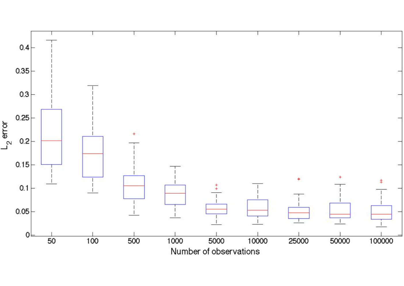
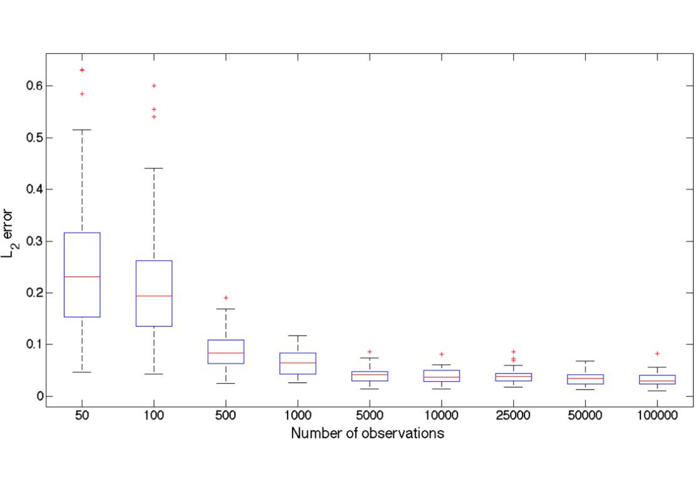
Figure 1 displays the L2\mathrm{L}^{2} error of the estimation of f⋆f_{\star} after 100100 iterations as a function of the number of observations. The L2\mathrm{L}^{2} estimation error decreases quickly for small values of nn (lower than 50005000) and then goes on decreasing at a lower rate as nn increases. It can be seen that even with a great number of observations, a small bias still remains for both functions (with a mean a bit lower than 0.050.05). Indeed, there are always small errors in the estimation of f⋆f_{\star} around x=0x=0 and x=1x=1.

Refer to caption
(a) f1f_{1}.
Refer to caption
(b) f2f_{2}.
Figure 1: L2\mathrm{L}^{2} error after 100100 iterations over 100100 Monte Carlo runs.

Figure 2 shows the estimates after 100100 iterations when n=25.000n=25.000. We observe on this Monte Carlo study that all the runs converge towards the isometric transformation x↦f⋆​(1−x)x\mapsto f_{\star}(1-x). This can be explained by the choice of the starting point of the EM algorithm. The isometry is used in Figure 1 to compute the L2\mathrm{L}^{2} error. This simulation illustrates the identifiability results obtained in Section 4.

(a) With no isometry for f1f_{1}.
(b) With the isometry x↦1−xx\mapsto 1-x for f1f_{1}.
Figure 2: True functions (bold lines) and estimates after 100100 iterations (vertical lines) over 100100 Monte Carlo runs (n=25.000n=25.000).

6.2.3 Experiment 2: (Xk)k≥0(X_{k})_{k\geq 0} Markov chain

In this section, b=2b=2 and a⋆a_{\star} and f⋆f_{\star} are estimated. Define for any a>0a>0,

νa​(x,x′)\displaystyle\nu_{a}(x,x^{\prime}) =ν1,a​(x)⋅ca​(x)​exp⁡(−|x−x′|a),\displaystyle=\nu_{1,a}(x)\cdot c_{a}(x)\exp\left(-\frac{|x-x^{\prime}|}{a}\right)\;,
ν1,a​(x)\displaystyle\nu_{1,a}(x) ∝ca−1​(x)=∫[0,1]exp⁡(−|x−x′|a)​d​x′.\displaystyle\propto c_{a}^{-1}(x)=\int_{[0,1]}\exp\left(-\frac{|x-x^{\prime}|}{a}\right)\mathrm{d}x^{\prime}\;.

ν^t+1\widehat{\nu}^{t+1} is given by νa^t+1\nu_{\widehat{a}^{t+1}} where a^t+1\widehat{a}^{t+1} is computed by maximizing the function

a↦log(a+a2(exp(−1/a)−1))+1n​a∑k=0n−1∑j=1Nm​cωkt,j|ξk,0t,j−ξk,1t,j|,a\mapsto\log\left(a+a^{2}(\exp(-1/a)-1)\right)+\frac{1}{na}\sum_{k=0}^{n-1}\sum_{j=1}^{N_{mc}}\omega_{k}^{t,j}|\xi_{k,0}^{t,j}-\xi_{k,1}^{t,j}|\;,

where, for all 0≤k≤n−10\leq k\leq n-1, (ξk,0t,j,ξk,1t,j)j=1Nm​c(\xi_{k,0}^{t,j},\xi_{k,1}^{t,j})_{j=1}^{N_{mc}} are independently sampled uniformly in [0,1]×[0,1][0,1]\times[0,1] and associated with the importance weights:

ωkt,j∝νa^t​(ξk,0t,j)​qa^t​(ξk,0t,j,ξk,1t,j)​φ​(Y2​k−f^t​(ξk,0t,j))​φ​(Y2​k+1−f^t​(ξk,1t,j)).\omega_{k}^{t,j}\propto\nu_{\widehat{a}^{t}}(\xi_{k,0}^{t,j})q_{\widehat{a}^{t}}(\xi_{k,0}^{t,j},\xi_{k,1}^{t,j})\varphi(Y_{2k}-\widehat{f}^{t}(\xi_{k,0}^{t,j}))\varphi(Y_{2k+1}-\widehat{f}^{t}(\xi_{k,1}^{t,j}))\;. (27)

The Monte Carlo approximations are computed using Nm​c=200N_{mc}=200 and 20.00020.000 observations (i.e. n=10.000n=10.000) are sampled. Figure 3 displays the estimation a⋆a_{\star} as a function of the number of iterations of the EM algorithm over 5050 independent Monte Carlo runs. The estimates converge to the true value of a⋆a_{\star} after few iterations (about 2525).

Figure 3: Estimation of a⋆a_{\star} as a function of the number of iterations of the EM algorithm. The true value is a⋆=1a_{\star}=1. Median (bold line) and upper and lower quartiles (dotted line) over 5050 Monte Carlo runs.

Figure 4 illustrates Corollary 5.2. It displays the estimation of f⋆​([0,1])f_{\star}([0,1]) after 100100 iterations for several Monte Carlo runs. It shows that despite the variability of the estimation, the image is well estimated with few observations.

Figure 4: True image f⋆​([0,1])f_{\star}([0,1]) (red) and estimates after 100100 iterations of the algorithm over 100100 Monte Carlo runs (grey).

7 Proofs

7.1 Proof of Proposition 3.2

Recall that for any probability density function pp on ℝb​ℓ\mathbb{R}^{b\ell}, gpg_{p} is defined in (12) by

gp=def12​ln⁡p+p⋆2​p⋆.g_{p}\stackrel{{\scriptstyle\mathrm{def}}}{{=}}\frac{1}{2}\ln\frac{p+p_{\star}}{2p_{\star}}\;.

The proof relies on the application of Proposition A.1 and Proposition A.2 to obtain first a concentration inequality for the class of functions 𝒢M\mathcal{G}_{M}, where M≥1M\geq 1, defined as:

𝒢M=def{gpf,ν;ν∈𝒟b,f∈ℱandI(f)≤M},\mathcal{G}_{M}\stackrel{{\scriptstyle\mathrm{def}}}{{=}}\left\{g_{p_{f,\nu}}\;;\;\nu\in\mathcal{D}_{b},\;f\in\mathcal{F}\;\mbox{and}\;I(f)\leq M\right\}\;,

where pf,νp_{f,\nu} is defined by (3). For any p>0p>0, denote by Lp​(ℙ⋆)\mathrm{L}^{p}(\mathbb{P}_{\star}) the set of functions g:ℝb​ℓ→ℝg:\mathbb{R}^{b\ell}\to\mathbb{R} such that 𝔼⁡[|g⁡(𝐘0)|p]<+∞\mathbb{E}\left[\left|g(\mathbf{Y}_{0})\right|^{p}\right]<+\infty. For any κ>0\kappa>0 and any set 𝒢\mathcal{G} of functions from ℝb​ℓ\mathbb{R}^{b\ell} to ℝ\mathbb{R}, let N[](κ,𝒢,∥⋅∥Lp​(ℙ⋆))N_{[]}(\kappa,\mathcal{G},\|\cdot\|_{\mathrm{L}^{p}(\mathbb{P}_{\star})}) be the smallest integer NN such that there exists a set of functions {(giL,giU)}i=1N\left\{\left(g^{L}_{i},g^{U}_{i}\right)\right\}_{i=1}^{N} for which:

  1. a)

    ‖giU−giL‖Lp​(ℙ⋆)≤κ\|g^{U}_{i}-g^{L}_{i}\|_{\mathrm{L}^{p}(\mathbb{P}_{\star})}\leq\kappa for all i∈{1,⋯,N}i\in\{1,\cdots,N\};

  2. b)

    for any gg in 𝒢\mathcal{G}, there exists i∈{1,⋯,N}i\in\left\{1,\cdots,N\right\} such that

    giL≤g≤giU.g_{i}^{L}\leq g\leq g_{i}^{U}\;.

N[](κ,𝒢,∥⋅∥Lp​(ℙ⋆))N_{[]}(\kappa,\mathcal{G},\|\cdot\|_{\mathrm{L}^{p}(\mathbb{P}_{\star})}) is the κ\kappa-number with bracketing of 𝒢\mathcal{G}, and H[](κ,𝒢,∥⋅∥Lp​(ℙ⋆))=deflnN[](κ,𝒢,∥⋅∥Lp​(ℙ⋆))H_{[]}(\kappa,\mathcal{G},\|\cdot\|_{\mathrm{L}^{p}(\mathbb{P}_{\star})})\stackrel{{\scriptstyle\mathrm{def}}}{{=}}\ln N_{[]}(\kappa,\mathcal{G},\|\cdot\|_{\mathrm{L}^{p}(\mathbb{P}_{\star})}) is the κ\kappa-entropy with bracketing of 𝒢\mathcal{G}. For any bounded function gg, define

Sn​(g)=defn​∫g​d​(ℙn−ℙ⋆)=∑k=0n−1g⁡(𝐘k)−n​𝔼​[g⁡(𝐘0)].S_{n}(g)\stackrel{{\scriptstyle\mathrm{def}}}{{=}}n\int g\,\mathrm{d}(\mathbb{P}_{n}-\mathbb{P}_{\star})=\sum_{k=0}^{n-1}g(\mathbf{Y}_{k})-n\mathbb{E}[g(\mathbf{Y}_{0})]\;. (28)
Application of Proposition A.1

Proposition A.1 is applied to the class of functions 𝒢¯M\overline{\mathcal{G}}_{M} defined as

𝒢¯M=def{g−𝔼⁡[g⁡(𝐘0)];g∈𝒢M}.\overline{\mathcal{G}}_{M}\stackrel{{\scriptstyle\mathrm{def}}}{{=}}\left\{g-\mathbb{E}\left[g(\mathbf{Y}_{0})\right];\;g\in\mathcal{G}_{M}\right\}\;.
  1. -

    By HH2, there exists C>0C>0 such that for any i≥0i\geq 0, and any g∈𝒢Mg\in\mathcal{G}_{M},

    |g⁡(𝐘i)|≤C​Mυ​(1+‖𝐘i‖)\displaystyle\left|g\left(\mathbf{Y}_{i}\right)\right|\leq CM^{\upsilon}\left(1+\|\mathbf{Y}_{i}\|\right) ≤CMυ(1+||𝐟⋆(𝐗i)∥+∥ϵi∥),\displaystyle\leq CM^{\upsilon}\left(1+||\mathbf{f_{\star}}(\mathbf{X}_{i})\|+\|\boldsymbol{\epsilon}_{i}\|\right)\;,
    ≤C​Mυ​(1+‖f⋆‖∞+‖ϵi‖),\displaystyle\leq CM^{\upsilon}\left(1+\|f_{\star}\|_{\infty}+\|\boldsymbol{\epsilon}_{i}\|\right)\;,
    ≤C​Mυ​(1+‖ϵi‖).\displaystyle\leq CM^{\upsilon}\left(1+\|\boldsymbol{\epsilon}_{i}\|\right)\;.

    Define 𝐔i=defC​Mυ​(1+‖ϵi‖)\mathbf{U}_{i}\stackrel{{\scriptstyle\mathrm{def}}}{{=}}CM^{\upsilon}\left(1+\|\boldsymbol{\epsilon}_{i}\|\right). Then, the random variables (𝐔i)i≥0(\mathbf{U}_{i})_{i\geq 0} are i.i.d. and for all i≥0i\geq 0, |g⁡(𝐘i)−𝔼⁡[g⁡(𝐘0)]|≤𝐔i+𝔼⁡[𝐔0]|g\left(\mathbf{Y}_{i}\right)-\mathbb{E}\left[g(\mathbf{Y}_{0})\right]|\leq\mathbf{U}_{i}+\mathbb{E}\left[\mathbf{U}_{0}\right]. Furthermore,

    𝔼⁡[(𝐔i+𝔼⁡[𝐔0])2​k]≤k!​ν​ck−1withν=defC​M2​υandc=defC​M2​υ.\mathbb{E}\left[(\mathbf{U}_{i}+\mathbb{E}\left[\mathbf{U}_{0}\right])^{2k}\right]\leq k!\nu c^{k-1}\quad\mbox{with}\quad\nu\stackrel{{\scriptstyle\mathrm{def}}}{{=}}CM^{2\upsilon}\quad\mbox{and}\quad c\stackrel{{\scriptstyle\mathrm{def}}}{{=}}CM^{2\upsilon}\;.
  2. -

    On the other hand, since the random variables (ϵk)k≥0(\boldsymbol{\epsilon}_{k})_{k\geq 0} are i.i.d. and (𝐗k)k≥0(\mathbf{X}_{k})_{k\geq 0} is Φ\Phi-mixing, (𝐘k)k≥0(\mathbf{Y}_{k})_{k\geq 0} is also Φ\Phi-mixing with mixing coefficients (ϕi𝐘)i≥0(\phi^{\mathbf{Y}}_{i})_{i\geq 0} satisfying, for all i≥1i\geq 1, ϕi𝐘≤ϕi𝐗=ϕ(i−1)​b+1X\phi^{\mathbf{Y}}_{i}\leq\phi^{\mathbf{X}}_{i}=\phi^{X}_{(i-1)b+1}. Therefore 𝚽𝐘=∑i≥1(ϕi𝐘)1/2<∞\mathbf{\Phi^{Y}}=\sum_{i\geq 1}(\phi_{i}^{\mathbf{Y}})^{1/2}<\infty.

By Proposition A.1, there exists a positive constant CC such that for any positive xx,

ℙ[supg∈𝒢M|Sn(g)|≥𝔼[supg∈𝒢M|Sn(g)|]+C𝚽𝐘×(n​x+x)Mυ]≤e−x.\mathbb{P}\left[\sup_{g\in\mathcal{G}_{M}}\left|S_{n}(g)\right|\geq\mathbb{E}\left[\sup_{g\in\mathcal{G}_{M}}\left|S_{n}(g)\right|\right]+C\mathbf{\Phi^{Y}}\times\left(\sqrt{nx}+x\right)M^{\upsilon}\right]\leq\mathrm{e}^{-x}\;. (29)
Application of Proposition A.2

Proposition A.2 is used to control the inner expectation in (29). Let r>1r>1. By [21, Lemma 7.26] and since the Hellinger distance is bounded by 11, there exists a constant δ\delta such that for any g=gpf,ν∈𝒢Mg=g_{p_{f,\nu}}\in\mathcal{G}_{M}.

‖g‖L2​r​(ℙ⋆)2​r≤δ.\|g\|^{2r}_{\mathrm{L}^{2r}(\mathbb{P}_{\star})}\leq\delta\;.

By Lemma B.1, for any q>1q>1, any s>b​ℓ/qs>b\ell/q and any β>s+b​ℓ​(1−1/q)\beta>s+b\ell(1-1/q), there exists a constant cc such that, for all u>0u>0,

H[](u,∥⋅∥L2​r​(ℙ⋆),𝒢M)≤c(Mυ⁡(s+β+b​ℓ/q)u2​r)b​ℓ/sH_{[]}(u,\|\cdot\|_{\mathrm{L}^{2r}(\mathbb{P}_{\star})},\mathcal{G}_{M})\leq c\left(\frac{M^{\upsilon(s+\beta+b\ell/q)}}{u^{2r}}\right)^{b\ell/s} (30)

and

φ(δ)=def∫0δH[]1/2(u,∥⋅∥L2​r​(ℙ⋆),𝒢M)du≤cM(s+β+b​ℓ/q)​b​ℓ​υ/(2​s)∫0δu−rbℓ/sdu.\varphi(\delta)\stackrel{{\scriptstyle\mathrm{def}}}{{=}}\int_{0}^{\delta}H_{[]}^{1/2}(u,\|\cdot\|_{\mathrm{L}^{2r}(\mathbb{P}_{\star})},\mathcal{G}_{M})\mathrm{d}u\leq cM^{(s+\beta+b\ell/q)b\ell\upsilon/(2s)}\int_{0}^{\delta}u^{-rb\ell/s}\mathrm{d}u\;.

Choosing β≤s+b​ℓ​(1−1/q)+2\beta\leq s+b\ell(1-1/q)+2, if ss goes to +∞+\infty then the last integral is finite, and (s+β+b​ℓ/q)​b​ℓ​υ/(2​s)(s+\beta+b\ell/q)b\ell\upsilon/(2s) converges to b​ℓ​υb\ell\upsilon, so that for any η>0\eta>0 there exists a positive constant cc such that

φ⁡(δ)≤c​Mb​ℓ​υ+η.\varphi(\delta)\leq cM^{b\ell\upsilon+\eta}\;.

Finally, by Proposition A.2 for any η>0\eta>0, there exists a constant AA such that for nn large enough

𝔼⁡[supg∈𝒢M|Sn​(g)|]≤A​n​Mb​ℓ​υ+η.\mathbb{E}\left[\sup_{g\in\mathcal{G}_{M}}\left|S_{n}(g)\right|\right]\leq A\sqrt{n}M^{b\ell\upsilon+\eta}\;.

Then, by (29), this yields

ℙ[supg∈𝒢M|Sn(g)|≥c𝚽𝐘×(n​x+x)Mυ+AnMb​ℓ​υ+η]≤e−x.\mathbb{P}\left[\sup_{g\in\mathcal{G}_{M}}|S_{n}(g)|\geq c\mathbf{\Phi^{Y}}\times\left(\sqrt{nx}+x\right)M^{\upsilon}+A\sqrt{n}M^{b\ell\upsilon+\eta}\right]\leq\mathrm{e}^{-x}\;. (31)

Proposition 3.2 is then proved using a peeling argument. By (28) and (31), for any M≥1M\geq 1, any large enough nn and any x>0x>0, if γ=b​ℓ​υ+η\gamma=b\ell\upsilon+\eta,

ℙ[supg∈𝒢M|∫g​d​(ℙn−ℙ⋆)|Mγ≥c𝚽𝐘×(xn+xn)+An]≤e−Mγ−υ​x.\mathbb{P}\left[\sup_{g\in\mathcal{G}_{M}}\frac{\left|\int g\ \mathrm{d}(\mathbb{P}_{n}-\mathbb{P}_{\star})\right|}{M^{\gamma}}\geq c\mathbf{\Phi^{Y}}\times\left(\sqrt{\frac{x}{n}}+\frac{x}{n}\right)+\frac{A}{\sqrt{n}}\right]\leq e^{-M^{\gamma-\upsilon}x}\;. (32)

We can write

ℙ[supf∈ℱ,ν∈𝒟b|∫gpf,ν​d​(ℙn−ℙ⋆)|1∨I​(f)γ≥c𝚽𝐘×(xn+xn)+2γ​An]≤P1+∑k=0+∞Tk,\mathbb{P}\left[\sup_{f\in\mathcal{F},\ \nu\in\mathcal{D}_{b}}\frac{\left|\int g_{p_{f,\nu}}\ \mathrm{d}(\mathbb{P}_{n}-\mathbb{P}_{\star})\right|}{1\vee I(f)^{\gamma}}\geq c\mathbf{\Phi^{Y}}\times\left(\sqrt{\frac{x}{n}}+\frac{x}{n}\right)+\frac{2^{\gamma}A}{\sqrt{n}}\right]\leq P_{1}+\sum_{k=0}^{+\infty}T_{k}\;,

where

P1\displaystyle P_{1} =defℙ[supf∈ℱ;I(f)≤1,ν∈𝒟b|∫gpf,ν​d​(ℙn−ℙ⋆)|1∨I​(f)γ≥c𝚽𝐘×(xn+xn)+2γ​An],\displaystyle\stackrel{{\scriptstyle\mathrm{def}}}{{=}}\mathbb{P}\left[\sup_{\begin{subarray}{c}f\in\mathcal{F};\;I(f)\leq 1,\\ \nu\in\mathcal{D}_{b}\end{subarray}}\frac{\left|\int g_{p_{f,\nu}}\ \mathrm{d}(\mathbb{P}_{n}-\mathbb{P}_{\star})\right|}{1\vee I(f)^{\gamma}}\geq c\mathbf{\Phi^{Y}}\times\left(\sqrt{\frac{x}{n}}+\frac{x}{n}\right)+\frac{2^{\gamma}A}{\sqrt{n}}\right]\;,
Tk\displaystyle T_{k} =defℙ[supf∈ℱ; 2k<I(f)≤2k+1,ν∈𝒟b|∫gpf,ν​d​(ℙn−ℙ⋆)|1∨I​(f)γ≥c𝚽𝐘×(xn+xn)+2γ​An].\displaystyle\stackrel{{\scriptstyle\mathrm{def}}}{{=}}\mathbb{P}\left[\sup_{\begin{subarray}{c}f\in\mathcal{F};\;2^{k}<I(f)\leq 2^{k+1},\\ \nu\in\mathcal{D}_{b}\end{subarray}}\frac{\left|\int g_{p_{f,\nu}}\ \mathrm{d}(\mathbb{P}_{n}-\mathbb{P}_{\star})\right|}{1\vee I(f)^{\gamma}}\geq c\mathbf{\Phi^{Y}}\times\left(\sqrt{\frac{x}{n}}+\frac{x}{n}\right)+\frac{2^{\gamma}A}{\sqrt{n}}\right]\;.

By (32),

P1≤ℙ[supg∈𝒢1|∫gd(ℙn−ℙ⋆)|≥c𝚽𝐘×(xn+xn)+2γ​An],≤ℙ[supg∈𝒢1|∫gd(ℙn−ℙ⋆)|≥c𝚽𝐘×(xn+c​xn)+An]≤e−xP_{1}\leq\mathbb{P}\left[\sup_{g\in\mathcal{G}_{1}}\left|\int g\ \mathrm{d}(\mathbb{P}_{n}-\mathbb{P}_{\star})\right|\geq c\mathbf{\Phi^{Y}}\times\left(\sqrt{\frac{x}{n}}+\frac{x}{n}\right)+\frac{2^{\gamma}A}{\sqrt{n}}\right]\;,\\ \leq\mathbb{P}\left[\sup_{g\in\mathcal{G}_{1}}\left|\int g\ \mathrm{d}(\mathbb{P}_{n}-\mathbb{P}_{\star})\right|\geq c\mathbf{\Phi^{Y}}\times\left(\sqrt{\frac{x}{n}}+\frac{\sqrt{c}x}{n}\right)+\frac{A}{\sqrt{n}}\right]\leq\mathrm{e}^{-x}

and for all k≥0k\geq 0,

Tk≤ℙ[supg∈𝒢2k+1|∫g​d​(ℙn−ℙ⋆)|2γ⁡(k+1)≥c2γ𝚽𝐘×(xn+xn)+An],≤ℙ[supg∈𝒢2k+1|∫g​d​(ℙn−ℙ⋆)|2γ⁡(k+1)≥c𝚽𝐘×(x22​γ​n+x22​γ​n)+An]≤e−2(γ−υ)​(k+1)x/22​γ.T_{k}\leq\mathbb{P}\left[\sup_{g\in\mathcal{G}_{2^{k+1}}}\frac{\left|\int g\ \mathrm{d}(\mathbb{P}_{n}-\mathbb{P}_{\star})\right|}{2^{\gamma(k+1)}}\geq\frac{c}{2^{\gamma}}\mathbf{\Phi^{Y}}\times\left(\sqrt{\frac{x}{n}}+\frac{x}{n}\right)+\frac{A}{\sqrt{n}}\right]\;,\\ \leq\mathbb{P}\left[\sup_{g\in\mathcal{G}_{2^{k+1}}}\frac{\left|\int g\ \mathrm{d}(\mathbb{P}_{n}-\mathbb{P}_{\star})\right|}{2^{\gamma(k+1)}}\geq c\mathbf{\Phi^{Y}}\times\left(\sqrt{\frac{x}{2^{2\gamma}n}}+\frac{x}{2^{2\gamma}n}\right)+\frac{A}{\sqrt{n}}\right]\leq\mathrm{e}^{-2^{(\gamma-\upsilon)(k+1)}x/2^{2\gamma}}\;.

Using (32),

ℙ[supf∈ℱ,ν∈𝒟b|∫gpf,ν​d​(ℙn−ℙ⋆)|1∨I​(f)γ\displaystyle\mathbb{P}\bigg[\sup_{f\in\mathcal{F},\ \nu\in\mathcal{D}_{b}}\frac{\left|\int g_{p_{f,\nu}}\ \mathrm{d}(\mathbb{P}_{n}-\mathbb{P}_{\star})\right|}{1\vee I(f)^{\gamma}} ≥c𝚽𝐘×(xn+xn)+2γ​An]\displaystyle\geq c\mathbf{\Phi^{Y}}\times\left(\sqrt{\frac{x}{n}}+\frac{x}{n}\right)+\frac{2^{\gamma}A}{\sqrt{n}}\bigg]
≤e−x+∑k=0∞e−2(γ−υ)​(k+1)x/22​γ\displaystyle\leq e^{-x}+\sum_{k=0}^{\infty}e^{-2^{(\gamma-\upsilon)(k+1)}x/2^{2\gamma}}
≤e−x+∑k=0∞e−(k+1)xlog(2)(γ−υ)/22​γ\displaystyle\leq e^{-x}+\sum_{k=0}^{\infty}e^{-(k+1)x\log(2)(\gamma-\upsilon)/2^{2\gamma}}
≤e−x+e−α​x1−e−α​x,\displaystyle\leq e^{-x}+\frac{e^{-\alpha x}}{1-e^{-\alpha x}}\;,

which concludes the proof of Proposition 3.2.

7.2 Proof of Proposition 4.1

Assume that h⁡(pf,ν,pf⋆,ν1,⋆)=0h(p_{f,\nu},p_{f_{\star},\nu_{1,\star}})=0 (the proof of the converse proposition is straightforward). Let X0′X^{\prime}_{0} be a random variable on 𝕏\mathbb{X} with distribution ν⁡(x)​μ​(d​x)\nu(x)\mu(\mathrm{d}x). Since ϵ0\epsilon_{0} is a Gaussian random variable, h⁡(pf,ν,pf⋆,ν1,⋆)=0h(p_{f,\nu},p_{f_{\star},\nu_{1,\star}})=0 implies that f⁡(X0′)f(X^{\prime}_{0}) has the same distribution as f⋆​(X0)f_{\star}(X_{0}).

Proof that ff and f⋆f_{\star} have the same image in ℝℓ\mathbb{R}^{\ell}.

Let y∈f⁡(𝕏)y\in f(\mathbb{X}), n≥1n\geq 1 and B⁡(y,n−1)B(y,n^{-1}) be the open Euclidean ball in ℝℓ\mathbb{R}^{\ell} centered at yy with radius n−1n^{-1}. As y∈f⁡(𝕏)y\in f(\mathbb{X}) and ff is continuous, there exists a nonempty open subset 𝒪\mathcal{O} of ℝm\mathbb{R}^{m} such that f−1​(B⁡(y,n−1))=𝒪∩𝕏f^{-1}(B(y,n^{-1}))=\mathcal{O}\cap\mathbb{X}. Since 𝕏∘¯=𝕏\overline{\overset{\circ}{\mathbb{X}}}=\mathbb{X}, 𝕏∘\overset{\circ}{\mathbb{X}} is not empty and so is the interior of f−1​(B⁡(y,n−1))f^{-1}(B(y,n^{-1})) (which is equal to 𝒪∩𝕏∘\mathcal{O}\cap\overset{\circ}{\mathbb{X}}). Therefore, μ⁡{f−1​(B⁡(y,n−1))}>0\mu\left\{f^{-1}\left(B\left(y,n^{-1}\right)\right)\right\}>0. Then, using that ν≥ν−\nu\geq\nu_{-} and that f⁡(X0′)f(X^{\prime}_{0}) has the same distribution as f⋆​(X0)f_{\star}(X_{0}),

ℙ{X0∈f⋆−1(B(y,n−1))}=ℙ{X0′∈f−1(B(y,n−1))}≥ν−μ{f−1(B(y,n−1))}>0,\mathbb{P}\!\left\{X_{0}\in f_{\star}^{-1}\left(B\left(y,n^{-1}\right)\right)\right\}\!=\mathbb{P}\!\left\{X^{\prime}_{0}\in f^{-1}\left(B\left(y,n^{-1}\right)\right)\right\}\!\geq\nu_{-}\,\mu\left\{f^{-1}\left(B\left(y,n^{-1}\right)\right)\right\}>0\;,

Hence, f⋆−1​(B⁡(y,n−1))f_{\star}^{-1}\left(B\left(y,n^{-1}\right)\right) is nonempty and for all n≥1n\geq 1, there exists xn∈𝕏x_{n}\in\mathbb{X} such that ‖y−f⋆​(xn)‖<n−1\|y-f_{\star}(x_{n})\|<n^{-1}. Moreover, for all n≥1n\geq 1, f⋆​(xn)f_{\star}(x_{n}) lies in the compact set f⋆​(𝕏)f_{\star}(\mathbb{X}). This implies that y∈f⋆​(𝕏)y\in f_{\star}(\mathbb{X}). The proof of the converse inclusion follows the same lines.

Proof that ϕ\phi is bijective.

Since f⁡(X0′)f(X^{\prime}_{0}) has the same distribution as f⋆​(X0)f_{\star}(X_{0}), X0X_{0} has the same distribution as ϕ⁡(X0′)\phi(X^{\prime}_{0}) where ϕ=deff⋆−1∘f\phi\stackrel{{\scriptstyle\mathrm{def}}}{{=}}f_{\star}^{-1}\circ f. By HH6 ϕ\phi exists and is 𝒞1\mathcal{C}^{1}. We prove that |Jϕ|>0|J_{\phi}|>0 using the following result due to [11, Theorem 2, p.99].

Lemma 7.1.

If ϕ:𝕏→𝕏\phi:\mathbb{X}\to\mathbb{X} is Lipschitz then, for any integrable function gg,

∫𝕏g⁡(x)​|Jϕ​(x)|​μ​(𝑑x)=∫𝕏∑x∈ϕ−1​({y})g⁡(x)​μ​(𝑑y).\int_{\mathbb{X}}g(x)\left|J_{\phi}(x)\right|\mu(\mathrm{d}x)=\int_{\mathbb{X}}\sum_{x\in\phi^{-1}(\{y\})}g(x)\mu(\mathrm{d}y)\;.

Define A=def{x∈𝕏;∀x′∈ϕ−1({x}),|Jϕ(x′)|>0}A\stackrel{{\scriptstyle\mathrm{def}}}{{=}}\left\{x\in\mathbb{X}\;;\;\forall x^{\prime}\in\phi^{-1}(\{x\}),\ |J_{\phi}(x^{\prime})|>0\right\}. Let h1h_{1} be a bounded measurable real function on 𝕏\mathbb{X} and define h=def𝟙A​h1h\stackrel{{\scriptstyle\mathrm{def}}}{{=}}\mathds{1}_{A}h_{1}. By Lemma 7.1,

𝔼⁡[h∘ϕ⁡(X0′)]\displaystyle\mathbb{E}\left[h\circ\phi(X^{\prime}_{0})\right] =∫𝕏h1​(ϕ⁡(x′))​𝟙A​(ϕ⁡(x′))​ν​(x′)​μ​(d​x′),\displaystyle=\int_{\mathbb{X}}h_{1}(\phi(x^{\prime}))\mathds{1}_{A}(\phi(x^{\prime}))\nu(x^{\prime})\mu(\mathrm{d}x^{\prime})\;,
=∫𝕏h1​(ϕ⁡(x′))​𝟙A​(ϕ⁡(x′))​ν⁡(x′)|Jϕ​(x′)|​|Jϕ​(x′)|​μ​(d​x′),\displaystyle=\int_{\mathbb{X}}h_{1}(\phi(x^{\prime}))\mathds{1}_{A}(\phi(x^{\prime}))\frac{\nu(x^{\prime})}{|J_{\phi}(x^{\prime})|}|J_{\phi}(x^{\prime})|\mu(\mathrm{d}x^{\prime})\;,
=∫𝕏h1​(x)​𝟙A​(x)​∑x′∈ϕ−1​({x})ν⁡(x′)|Jϕ​(x′)|​μ​(𝑑x).\displaystyle=\int_{\mathbb{X}}h_{1}(x)\mathds{1}_{A}(x)\sum_{x^{\prime}\in\phi^{-1}(\{x\})}\frac{\nu(x^{\prime})}{|J_{\phi}(x^{\prime})|}\mu(\mathrm{d}x)\;.

Since X0X_{0} has the same distribution as ϕ⁡(X0′)\phi(X^{\prime}_{0}),

∫𝕏h1​(x)​𝟙A​(x)​ν1,⋆​(x)​μ​(𝑑x)=∫𝕏h1​(x)​𝟙A​(x)​∑x′∈ϕ−1​({x})ν⁡(x′)|Jϕ​(x′)|​μ​(𝑑x).\int_{\mathbb{X}}h_{1}(x)\mathds{1}_{A}(x)\nu_{1,\star}(x)\mu(\mathrm{d}x)=\int_{\mathbb{X}}h_{1}(x)\mathds{1}_{A}(x)\sum_{x^{\prime}\in\phi^{-1}(\{x\})}\frac{\nu(x^{\prime})}{|J_{\phi}(x^{\prime})|}\mu(\mathrm{d}x)\;.

Applying Lemma 7.1 with g=def𝟙|Jϕ|=0g\stackrel{{\scriptstyle\mathrm{def}}}{{=}}\mathds{1}_{|J_{\phi}|=0} implies that 𝟙A=1\mathds{1}_{A}=1 μ\mu-a.s. in 𝕏\mathbb{X} and, μ\mu-a.s.,

ν1,⋆​(x)=∑x′∈ϕ−1​({x})ν⁡(x′)|Jϕ​(x′)|.\nu_{1,\star}(x)=\sum_{x^{\prime}\in\phi^{-1}(\{x\})}\frac{\nu(x^{\prime})}{|J_{\phi}(x^{\prime})|}\;. (33)

Therefore, for μ\mu almost every x∈𝕏x\in\mathbb{X} and for all x′∈ϕ−1​({x})x^{\prime}\in\phi^{-1}(\{x\}),

|Jϕ​(x′)|≥ν−ν+.|J_{\phi}(x^{\prime})|\geq\frac{\nu_{-}}{\nu_{+}}\;.

By continuity of JϕJ_{\phi} and using that 𝕏∘¯=𝕏\overline{\overset{\circ}{\mathbb{X}}}=\mathbb{X}, |Jϕ​(x)|>0|J_{\phi}(x)|>0 for all x∈𝕏x\in\mathbb{X}. Therefore, ϕ\phi is locally invertible and, since 𝕏\mathbb{X} is compact, simply connected and arcwise connected, ϕ\phi is bijective by [2, Theorem 1.81.8, p.4747]. Then (33) ensures that for μ\mu almost every x∈𝕏x\in\mathbb{X},

ν1,⋆​(ϕ⁡(x))=ν⁡(x)|Jϕ​(x)|,\nu_{1,\star}(\phi(x))=\frac{\nu(x)}{|J_{\phi}(x)|}\;,

which concludes the proof of Proposition 4.1.

7.3 Proof of Proposition 4.3 and Corollary 4.4

Proof of Proposition 4.3

The proof of (18) follows the same lines as the proof of Proposition 4.1. Let (X0′,X1′)(X^{\prime}_{0},X^{\prime}_{1}) be a random variable on 𝕏2\mathbb{X}^{2} with probability density ν⁡(x)​q​(x,x′)\nu(x)q(x,x^{\prime}) on 𝕏2\mathbb{X}^{2}. h⁡(pf,ν2,pf⋆,ν2,⋆)=0h(p_{f,\nu^{2}},p_{f_{\star},\nu_{2,\star}})=0 implies that h⁡(pf,ν,pf⋆,ν⋆)=0h(p_{f,\nu},p_{f_{\star},\nu_{\star}})=0 and, by Proposition 4.1, f​(𝕏)=f⋆​(𝕏)f(\mathbb{X})=f_{\star}(\mathbb{X}) and ϕ=f⋆−1∘f\phi=f_{\star}^{-1}\circ f is bijective. Moreover, since (ϵ0,ϵ1)(\epsilon_{0},\epsilon_{1}) has a Gaussian distribution, h⁡(pf,ν2,pf⋆,ν⋆2)=0h(p_{f,\nu^{2}},p_{f_{\star},\nu_{\star}^{2}})=0 implies that (ϕ⁡(X0′),ϕ⁡(X1′))(\phi(X^{\prime}_{0}),\phi(X^{\prime}_{1})) has the same distribution as (X0,X1)(X_{0},X_{1}) so that for any xx in 𝕏\mathbb{X} and any bounded measurable function ff on 𝕏\mathbb{X},

𝔼⁡[ϕ⁡(X1′)|X0′=ϕ−1​(x)]=𝔼⁡[X1|X0=x].\mathbb{E}\left[\phi(X^{\prime}_{1})\middle|X^{\prime}_{0}=\phi^{-1}(x)\right]=\mathbb{E}\left[X_{1}\middle|X_{0}=x\right]\;.

Following the proof of Proposition 4.1, this gives (18).

Proof of Corollary 4.4

Assume that

q⋆​(x,x′)=c⋆​(x)​ρ⋆​(‖x−x′‖)andq⁡(x,x′)=c⁡(x)​ρ​(‖x−x′‖).q_{\star}(x,x^{\prime})=c_{\star}(x)\rho_{\star}(||x-x^{\prime}||)\quad\mbox{and}\quad q(x,x^{\prime})=c(x)\rho(||x-x^{\prime}||)\;.

By (18),

c⁡(x)​ρ​(‖x−x′‖)=|Jϕ​(x′)|​c⋆​(ϕ⁡(x))​ρ⋆​(‖ϕ⁡(x)−ϕ⁡(x′)‖).c(x)\rho(||x-x^{\prime}||)=|J_{\phi}(x^{\prime})|c_{\star}(\phi(x))\rho_{\star}(||\phi(x)-\phi(x^{\prime})||)\;. (34)

Applying (34) with x=x′x=x^{\prime} implies |Jϕ​(x)|=ρ⁡(0)ρ⋆​(0)​c⁡(x)c⋆​(ϕ​(x))|J_{\phi}(x)|=\frac{\rho(0)}{\rho_{\star}(0)}\frac{c(x)}{c_{\star}(\phi(x))}. Therefore,

|Jϕ​(x)||Jϕ​(x′)|=c⁡(x)​c⋆​(ϕ⁡(x′))c⁡(x′)​c⋆​(ϕ⁡(x))=|Jϕ​(x′)||Jϕ​(x)|\frac{|J_{\phi}(x)|}{|J_{\phi}(x^{\prime})|}=\frac{c(x)c_{\star}(\phi(x^{\prime}))}{c(x^{\prime})c_{\star}(\phi(x))}=\frac{|J_{\phi}(x^{\prime})|}{|J_{\phi}(x)|}

and then, there exists a constant CC such that for all x∈𝕏x\in\mathbb{X}, |Jϕ​(x)|=C|J_{\phi}(x)|=C. As ϕ\phi is bijective we may write

μ⁡(𝕏)=μ⁡(ϕ⁡(𝕏))=∫ϕ⁡(𝕏)μ⁡(𝑑x)=∫𝕏|Jϕ​(x)|​μ​(𝑑x)=C​μ​(𝕏),\mu(\mathbb{X})=\mu(\phi(\mathbb{X}))=\int_{\phi(\mathbb{X})}\mu(\mathrm{d}x)=\int_{\mathbb{X}}|J_{\phi}(x)|\mu(\mathrm{d}x)=C\mu(\mathbb{X})\;,

which leads to C=1C=1 since 0<μ⁡(𝕏)<∞0<\mu(\mathbb{X})<\infty. By (34), for any xx and x′x^{\prime} in 𝕏\mathbb{X},

ρ⁡(‖x−x′‖)=ρ⋆​(‖ϕ⁡(x)−ϕ⁡(x′)‖).\rho(||x-x^{\prime}||)=\rho_{\star}(||\phi(x)-\phi(x^{\prime})||). (35)

Let x0∈𝕏∘x_{0}\in\overset{\circ}{\mathbb{X}}, y0=ϕ⁡(x0)y_{0}=\phi(x_{0}) and d0,d0′>0d_{0},d_{0}^{\prime}>0 be such that B⁡(x0,d0)=def{x∈ℝm,‖x0−x‖<d0}⊂𝕏B(x_{0},d_{0})\stackrel{{\scriptstyle\mathrm{def}}}{{=}}\{x\in\mathbb{R}^{m}\;,\;||x_{0}-x||<d_{0}\}\subset\mathbb{X} and ϕ⁡(B⁡(x0,d0))⊂B⁡(y0,d0′)\phi(B(x_{0},d_{0}))\subset B(y_{0},d_{0}^{\prime}).

Let d<d0d<d_{0} and denote by S⁡(x0,d)S(x_{0},d) the set S⁡(x0,d)=def{x∈ℝm,‖x0−x‖=d}S(x_{0},d)\stackrel{{\scriptstyle\mathrm{def}}}{{=}}\{x\in\mathbb{R}^{m}\;,\;||x_{0}-x||=d\}. As ρ⋆\rho_{\star} is one-to-one, write F=ρ⋆−1∘ρF=\rho_{\star}^{-1}\circ\rho. (35) implies that ϕ⁡(S⁡(x0,d))⊂S⁡(y0,F⁡(d))\phi(S(x_{0},d))\subset S(y_{0},F(d)). Furthermore, using the compactness and the connectivity of S⁡(x0,d)S(x_{0},d), ϕ⁡(S⁡(x0,d))=S⁡(y0,F⁡(d))\phi(S(x_{0},d))=S(y_{0},F(d)) which, together with the continuity of ϕ\phi, guarantees that ϕ⁡(B⁡(x0,d))=B⁡(y0,F⁡(d))\phi(B(x_{0},d))=B(y_{0},F(d)). Finally, because ϕ\phi preserves the volumes, for any d<d0d<d_{0}, F⁡(d)=dF(d)=d and for any x∈𝕏x\in\mathbb{X} and any x′∈B⁡(x,d0)x^{\prime}\in B(x,d_{0}), ‖x−x′‖=‖ϕ⁡(x)−ϕ⁡(x′)‖||x-x^{\prime}||=||\phi(x)-\phi(x^{\prime})||. The proof is concluded using the connectivity of 𝕏\mathbb{X}.

Appendix A Concentration results for the empirical process of unbounded functions

Proposition A.1 provides a concentration inequality on the empirical process over a class of functions 𝒢\mathcal{G} for which |g⁡(Zi)||g(Z_{i})| can be bounded uniformly in g∈𝒢g\in\mathcal{G} by an independent process UiU_{i} with bounded moments. This unusual condition is more general than [24, Theorem 3] which considered a uniformly bounded class of functions.

Proposition A.1.

Let (Zn)n≥0(Z_{n})_{n\geq 0} be a Φ\Phi-mixing process taking values in a set 𝒵\mathcal{Z}. Assume that the Φ\Phi-mixing coefficients associated with (Zn)n≥0(Z_{n})_{n\geq 0} satisfy:

𝚽=def∑i=1∞ϕi1/2<∞.\mathbf{\Phi}\stackrel{{\scriptstyle\mathrm{def}}}{{=}}\sum_{i=1}^{\infty}\phi_{i}^{1/2}<\infty\;.

Let 𝒢\mathcal{G} be some countable class of real valued measurable functions defined on 𝒵\mathcal{Z}. Assume that there exists a sequence of independent random variables (Ui)i≥0(U_{i})_{i\geq 0} such that:

  1. -

    for any gg in 𝒢\mathcal{G} ,

    |g⁡(Zi)|≤Ui​a.s.;|g(Z_{i})|\leq U_{i}\ a.s.\;; (36)
  2. -

    there exists some positive numbers ν\nu and cc such that, for any k≥1k\geq 1:

    ∑i=0n−1𝔼⁡[Ui2​k]≤k!​n​ν​ck−1.\sum_{i=0}^{n-1}\mathbb{E}\left[U_{i}^{2k}\right]\leq k!n\nu c^{k-1}\;. (37)

Then, for any positive xx,

ℙ[Sn≥2𝚽×(2n​ν​x+cx)]≤e−x,\mathbb{P}\left[S_{n}\geq 2\mathbf{\Phi}\times\left(2\sqrt{n\nu x}+\sqrt{c}x\right)\right]\leq\mathrm{e}^{-x}\;,

where

Sn=supg∈𝒢|∑i=0n−1g⁡(Zi)|−𝔼⁡[supg∈𝒢|∑i=0n−1g⁡(Zi)|].S_{n}=\sup_{g\in\mathcal{G}}\left|\sum_{i=0}^{n-1}g(Z_{i})\right|-\mathbb{E}\left[\sup_{g\in\mathcal{G}}\left|\sum_{i=0}^{n-1}g(Z_{i})\right|\right]\;.
Proof.

For any real valued random variable and for any real random variable XX, define ψX​(λ)=defln⁡(𝔼⁡[exp⁡(λ​X)])\psi_{X}(\lambda)\stackrel{{\scriptstyle\mathrm{def}}}{{=}}\ln\left(\mathbb{E}\left[\exp\left(\lambda X\right)\right]\right), Following the proof of [24, Theorem 3] together with the discussion about the dependence structure in [24, Section 2], we have

exp⁡(ψSn​(λ4))≤𝔼​[exp⁡[λ2​𝚽24​V2]]12​exp⁡[λ2​𝚽28​𝔼​[V2]],\exp\left(\psi_{S_{n}}\left(\frac{\lambda}{4}\right)\right)\leq\mathbb{E}\left[\exp\left[\lambda^{2}\frac{\mathbf{\Phi}^{2}}{4}V^{2}\right]\right]^{\frac{1}{2}}\exp\left[\lambda^{2}\frac{\mathbf{\Phi}^{2}}{8}\mathbb{E}\left[V^{2}\right]\right]\;, (38)

where V2=def∑i=1nUi2V^{2}\stackrel{{\scriptstyle\mathrm{def}}}{{=}}\sum_{i=1}^{n}U_{i}^{2}. Using (36) and by independence of the (Ui)i≥0(U_{i})_{i\geq 0},

exp⁡(ψSn​(λ4))\displaystyle\exp\left(\psi_{S_{n}}\left(\frac{\lambda}{4}\right)\right) ≤𝔼​[exp⁡[λ2​𝚽24​∑i=1nUi2]]12​exp⁡[λ2​𝚽28​∑i=1n𝔼⁡[Ui2]],\displaystyle\leq\mathbb{E}\left[\exp\left[\lambda^{2}\frac{\mathbf{\Phi}^{2}}{4}\sum_{i=1}^{n}U_{i}^{2}\right]\right]^{\frac{1}{2}}\exp\left[\lambda^{2}\frac{\mathbf{\Phi}^{2}}{8}\sum_{i=1}^{n}\mathbb{E}[U_{i}^{2}]\right]\;,
≤∏i=1n𝔼​[exp⁡[λ2​𝚽24​Ui2]]12​exp⁡[λ2​𝚽28​∑i=1n𝔼⁡[Ui2]].\displaystyle\leq\prod_{i=1}^{n}\mathbb{E}\left[\exp\left[\lambda^{2}\frac{\mathbf{\Phi}^{2}}{4}U_{i}^{2}\right]\right]^{\frac{1}{2}}\exp\left[\lambda^{2}\frac{\mathbf{\Phi}^{2}}{8}\sum_{i=1}^{n}\mathbb{E}[U_{i}^{2}]\right]\;.

Thus,

ψSn​(λ/4)≤12​∑i=1nln⁡{𝔼⁡[exp⁡(λ2​𝚽24​Ui2)]}+λ2​𝚽28​∑i=1n𝔼⁡[Ui2].\psi_{S_{n}}(\lambda/4)\leq\frac{1}{2}\sum_{i=1}^{n}\ln\left\{\mathbb{E}\left[\exp\left(\lambda^{2}\frac{\mathbf{\Phi}^{2}}{4}U_{i}^{2}\right)\right]\right\}+\lambda^{2}\frac{\mathbf{\Phi}^{2}}{8}\sum_{i=1}^{n}\mathbb{E}\left[U_{i}^{2}\right]\;.

Since for any u>0u>0, ln⁡(u)≤u−1\ln(u)\leq u-1, this yields

ψSn​(λ/4)≤12​∑k=1∞1k!​[λ2​𝚽24]k​∑i=1n𝔼⁡[Ui2​k]+λ2​𝚽28​∑i=1n𝔼⁡[Ui2].\psi_{S_{n}}(\lambda/4)\leq\frac{1}{2}\sum_{k=1}^{\infty}\frac{1}{k!}\left[\lambda^{2}\frac{\mathbf{\Phi}^{2}}{4}\right]^{k}\sum_{i=1}^{n}\mathbb{E}\left[U_{i}^{2k}\right]+\lambda^{2}\frac{\mathbf{\Phi}^{2}}{8}\sum_{i=1}^{n}\mathbb{E}\left[U_{i}^{2}\right]\;.

Then, by (37),

ψSn​(λ/4)≤n​ν​[λ2​𝚽24]​12​∑k=0∞[λ2​𝚽24​c]k+[λ2​𝚽28​ν].\psi_{S_{n}}(\lambda/4)\leq n\nu\left[\lambda^{2}\frac{\mathbf{\Phi}^{2}}{4}\right]\frac{1}{2}\sum_{k=0}^{\infty}\left[\lambda^{2}\frac{\mathbf{\Phi}^{2}}{4}c\right]^{k}+\left[\lambda^{2}\frac{\mathbf{\Phi}^{2}}{8}\nu\right]\;.

If 0<λ2​𝚽2​c/4<10<\lambda^{2}\mathbf{\Phi}^{2}c/4<1,

ψSn​(λ/4)\displaystyle\psi_{S_{n}}(\lambda/4) ≤n​ν​λ2​𝚽28​11−λ2​𝚽24​c+n​ν​λ2​𝚽28,\displaystyle\leq n\nu\lambda^{2}\frac{\mathbf{\Phi}^{2}}{8}\frac{1}{1-\lambda^{2}\frac{\mathbf{\Phi}^{2}}{4}c}+n\nu\lambda^{2}\frac{\mathbf{\Phi}^{2}}{8}\;,
≤n​ν​λ2​𝚽24​11−λ2​𝚽24​c.\displaystyle\leq n\nu\lambda^{2}\frac{\mathbf{\Phi}^{2}}{4}\frac{1}{1-\lambda^{2}\frac{\mathbf{\Phi}^{2}}{4}c}\;.

Define ν′=def8​n​ν​𝚽2\nu^{\prime}\stackrel{{\scriptstyle\mathrm{def}}}{{=}}8n\nu\mathbf{\Phi}^{2} and c′=def2​𝚽​cc^{\prime}\stackrel{{\scriptstyle\mathrm{def}}}{{=}}2\mathbf{\Phi}\sqrt{c}. Therefore,

ψSn​(λ/4)≤ν′​(λ/4)22​(1−c′​(λ/4)).\psi_{S_{n}}(\lambda/4)\leq\frac{\nu^{\prime}(\lambda/4)^{2}}{2(1-c^{\prime}(\lambda/4))}\;. (39)

Hence, for all 0<λ<1/c′0<\lambda<1/c^{\prime},

ψSn​(λ)≤ν′​λ22​(1−c′​λ).\psi_{S_{n}}(\lambda)\leq\frac{\nu^{\prime}\lambda^{2}}{2(1-c^{\prime}\lambda)}\;. (40)

By the Bernstein type inequality (40), [21, Lemma 2.3] gives, for any measurable set A⊂ΩA\subset\Omega with ℙ⁡(A)>0\mathbb{P}(A)>0,

𝔼⁡[Sn|A]≤2​ν′​ln⁡(1ℙ⁡(A))+c′​ln⁡(1ℙ⁡(A)).\mathbb{E}\left[S_{n}|A\right]\leq\sqrt{2\nu^{\prime}\ln\left(\frac{1}{\mathbb{P}(A)}\right)}+c^{\prime}\ln\left(\frac{1}{\mathbb{P}(A)}\right)\;.

Hence, by [21, Lemma 2.4], for any positive xx,

ℙ[Sn≥2​ν′​x+c′x]≤e−x.\mathbb{P}\left[S_{n}\geq\sqrt{2\nu^{\prime}x}+c^{\prime}x\right]\leq\mathrm{e}^{-x}\;.

∎

Proposition A.2 below provides a control on the expectation of the empirical process. It introduces a β\beta-mixing condition (see [7]) which is weaker than the Φ\Phi-mixing condition considered in Proposition A.1. The β\beta-mixing coefficient between two σ\sigma-fields 𝒰,𝒱⊂ℰ\mathcal{U},\mathcal{V}\subset\mathcal{E} is defined in [7] by

β⁡(𝒰,𝒱)=def12​sup∑(i,j)∈I×J|ℙ⁡(Ui∩Vj)−ℙ⁡(Ui)​ℙ​(Vj)|,\beta(\mathcal{U},\mathcal{V})\stackrel{{\scriptstyle\mathrm{def}}}{{=}}\frac{1}{2}\sup\sum_{(i,j)\in I\times J}\left|\mathbb{P}\left(U_{i}\cap V_{j}\right)-\mathbb{P}(U_{i})\mathbb{P}(V_{j})\right|\;,

where the supremum is taken over all finite partitions (Ui)i∈I(U_{i})_{i\in I} and (Vj)j∈J(V_{j})_{j\in J} respectively 𝒰\mathcal{U} and 𝒱\mathcal{V} measurable. The corresponding mixing coefficients (βi)i≥0(\beta_{i})_{i\geq 0} associated with a process (Xk)k≥0(X_{k})_{k\geq 0} satisfy βi<ϕi\beta_{i}<\phi_{i} for all i≥1i\geq 1.

Proposition A.2.

Let (Zi)i≥0(Z_{i})_{i\geq 0} be a stationary process taking values in a Polish space 𝒵\mathcal{Z} and let ℙ⋆\mathbb{P}_{\star} be the distribution of Z0Z_{0}. Assume that the sequence (Zi)i≥0(Z_{i})_{i\geq 0} is β\beta-mixing and that

∑i=1∞βi<∞.\sum_{i=1}^{\infty}\beta_{i}<\infty\;.

Let 𝒢\mathcal{G} be a countable class of functions on 𝒵\mathcal{Z}. Assume that there exist r>1r>1 and δ>0\delta>0 such that for any g∈𝒢g\in\mathcal{G},

‖g‖L2​r​(ℙ⋆)=def𝔼​[g​(Z0)2​r]1/2​r≤δ.||g||_{\mathrm{L}^{2r}(\mathbb{P}_{\star})}\stackrel{{\scriptstyle\mathrm{def}}}{{=}}\mathbb{E}\left[g(Z_{0})^{2r}\right]^{1/2r}\leq\delta\;.

Assume also that the bracketing function satisfies

∫01H[](u,||⋅||L2​r​(ℙ⋆),𝒢)​𝑑u<∞.\int_{0}^{1}\sqrt{H_{[]}(u,||\cdot||_{\mathrm{L}^{2r}(\mathbb{P}_{\star})},\mathcal{G})}\mathrm{d}u<\infty\;.

Then,

φ⁡(δ):=∫0δH[](u,||⋅||L2​r​(ℙ⋆),𝒢)​𝑑u\varphi(\delta):=\int_{0}^{\delta}\sqrt{H_{[]}(u,||\cdot||_{\mathrm{L}^{2r}(\mathbb{P}_{\star})},\mathcal{G})}\mathrm{d}u

is finite and there exists a constant AA such that for nn big enough

𝔼⁡[supg∈𝒢|Sn​(g)|]≤n​A​φ​(δ),\mathbb{E}\left[\sup_{g\in\mathcal{G}}|S_{n}(g)|\right]\leq\sqrt{n}A\varphi(\delta)\;, (41)

where, for all g∈𝒢g\in\mathcal{G}, Sn​(g)=∑i=0n−1g⁡(Zi)−n​𝔼​[g⁡(Z0)]S_{n}(g)=\sum_{i=0}^{n-1}g(Z_{i})-n\mathbb{E}\left[g(Z_{0})\right].

Proof.

This is a direct application of the remark following [9, Theorem 3]. ∎

Appendix B Entropy of the class 𝒢M\mathcal{G}_{M}

Lemma B.1.

For any q>1q>1, any s>b​ℓ/qs>b\ell/q and any even integer β\beta, provided that β>s+b​ℓ​(1−1/q)\beta>s+b\ell(1-1/q), there exists a constant CC such that for all u>0u>0,

H[](u,||⋅||L2​r​(ℙ⋆),𝒢M)≤C(Mυ⁡(s+β+b​ℓ/q)u2​r)b​ℓ/s.H_{[]}(u,||\cdot||_{\mathrm{L}^{2r}(\mathbb{P}_{\star})},\mathcal{G}_{M})\leq C\left(\frac{M^{\upsilon(s+\beta+b\ell/q)}}{u^{2r}}\right)^{b\ell/s}\;. (42)
Proof.

By [21, Lemma 7.26], for any probability densities p1p_{1} and p2p_{2} on ℝb​ℓ\mathbb{R}^{b\ell},

‖gp2−gp1‖L2​r​(ℙ⋆)2​r\displaystyle||g_{p_{2}}-g_{p_{1}}||^{2r}_{\mathrm{L}^{2r}(\mathbb{P}_{\star})} ≤C​‖p2−p1‖L2​(ℝb​ℓ)2.\displaystyle\leq C||\sqrt{p_{2}}-\sqrt{p_{1}}||^{2}_{\mathrm{L}^{2}(\mathbb{R}^{b\ell})}\;.

Since ‖p2−p1‖L2​(ℝb​ℓ)2≤‖p2−p1‖L1​(ℝb​ℓ)||\sqrt{p_{2}}-\sqrt{p_{1}}||^{2}_{\mathrm{L}^{2}(\mathbb{R}^{b\ell})}\leq||p_{2}-p_{1}||_{\mathrm{L}^{1}(\mathbb{R}^{b\ell})}, this yields, for any u>0u>0,

H[](u,||⋅||L2​r​(ℙ⋆),𝒢M)≤H[](u2​r/C,||⋅||L1​(ℝb​ℓ),𝒫M),H_{[]}(u,||\cdot||_{\mathrm{L}^{2r}(\mathbb{P}_{\star})},\mathcal{G}_{M})\leq H_{[]}\left(u^{2r}/C,||\cdot||_{\mathrm{L}^{1}(\mathbb{R}^{b\ell})},\mathcal{P}_{M}\right)\;, (43)

where 𝒫M=def{pf,ν;ν∈𝒟b,f∈ℱandI(f)≤M}\mathcal{P}_{M}\stackrel{{\scriptstyle\mathrm{def}}}{{=}}\left\{p_{f,\nu};\;\nu\in\mathcal{D}_{b},\;f\in\mathcal{F}\;\mbox{and}\;I(f)\leq M\right\}. Thus, it remains to bound the entropy with bracketing of 𝒫M\mathcal{P}_{M} associated with ||⋅||L1​(ℝb​ℓ)||\cdot||_{\mathrm{L}^{1}(\mathbb{R}^{b\ell})} to control the entropy with bracketing of 𝒢M\mathcal{G}_{M} associated with ||⋅||L2​r​(ℙ⋆)||\cdot||_{\mathrm{L}^{2r}(\mathbb{P}_{\star})}. For any q>1q>1 and s≥0s\geq 0, define the Sobolev space on ℝb​ℓ\mathbb{R}^{b\ell}:

Ws,q(ℝb​ℓ,ℝ)=def{h:ℝb​ℓ→ℝ;Dαh∈Lq,α∈ℕb​ℓand 0≤|α|≤s}.W^{s,q}\left(\mathbb{R}^{b\ell},\mathbb{R}\right)\stackrel{{\scriptstyle\mathrm{def}}}{{=}}\left\{h:\mathbb{R}^{b\ell}\to\mathbb{R};\;\;D^{\alpha}h\in\mathrm{L}^{q},\alpha\in\mathbb{N}^{b\ell}\;\mbox{and}\;0\leq|\alpha|\leq s\right\}\;.

For any β>0\beta>0, let ⟨⋅⟩β\langle\cdot\rangle^{\beta} be the polynomial function on ℝb​ℓ\mathbb{R}^{b\ell} given by 𝐲↦⟨𝐲⟩β=def(1+‖𝐲‖2)β/2\mathbf{y}\mapsto\langle\mathbf{y}\rangle^{\beta}\stackrel{{\scriptstyle\mathrm{def}}}{{=}}\left(1+\|\mathbf{y}\|^{2}\right)^{\beta/2} and Ws,q​(ℝb​ℓ,⟨⋅⟩β)W^{s,q}\left(\mathbb{R}^{b\ell},\langle\cdot\rangle^{\beta}\right) be the corresponding weighted Sobolev space:

Ws,q(ℝb​ℓ,⟨⋅⟩β)=def{h:ℝb​ℓ→ℝ;𝐲↦⟨𝐲⟩βh(𝐲)∈Ws,q(ℝb​ℓ,ℝ)}.W^{s,q}\left(\mathbb{R}^{b\ell},\langle\cdot\rangle^{\beta}\right)\stackrel{{\scriptstyle\mathrm{def}}}{{=}}\left\{h:\mathbb{R}^{b\ell}\to\mathbb{R};\;\ \mathbf{y}\mapsto\langle\mathbf{y}\rangle^{\beta}h(\mathbf{y})\in W^{s,q}\left(\mathbb{R}^{b\ell},\mathbb{R}\right)\right\}\;.

Lemma B.2 establishes that, for any M≥1M\geq 1, q>1q>1, s>b​ℓ/qs>b\ell/q and even integer β\beta, the normalized classes of functions 𝒫M/Mυ⁡(s+β+b​ℓ/q)\mathcal{P}_{M}/M^{\upsilon(s+\beta+b\ell/q)} are in the same bounded subspace of Ws,q​(ℝb​ℓ,⟨𝐲⟩β)W^{s,q}(\mathbb{R}^{b\ell},\langle\mathbf{y}\rangle^{\beta}). By [23, Corollary 4], for any q>1q>1, and any s>b​ℓ/qs>b\ell/q, provided that β>s+b​ℓ​(1−1/q)\beta>s+b\ell(1-1/q), there exists a constant CC such that, for all ϵ>0\epsilon>0,

H[](ϵ,∥⋅∥L1​(ℝb​ℓ),𝒫M/Mυ⁡(s+β+b​ℓ/q))≤Cϵ−bℓ/s.H_{[]}\left(\epsilon,\|\cdot\|_{\mathrm{L}^{1}(\mathbb{R}^{b\ell})},\mathcal{P}_{M}/M^{\upsilon(s+\beta+b\ell/q)}\right)\leq C\epsilon^{-b\ell/s}\;.

The proof is concluded by (43). ∎

Lemma B.2.

Assume that HH2 holds for some υ>0\upsilon>0. Then, for any q>1q>1, s>b​ℓ/qs>b\ell/q and any even β>0\beta>0, there exists C>0C>0 such that for any f∈ℱf\in\mathcal{F} and any ν∈𝒟b\nu\in\mathcal{D}_{b},

∥𝐲↦⟨𝐲⟩βpf,ν(𝐲)∥Ws,q​(ℝb​ℓ,ℝ)≤C(1∨I(f)υ)s+β+b​ℓ/q.\|\mathbf{y}\mapsto\langle\mathbf{y}\rangle^{\beta}p_{f,\nu}(\mathbf{y})\|_{W^{s,q}(\mathbb{R}^{b\ell},\mathbb{R})}\leq C(1\vee I(f)^{\upsilon})^{s+\beta+b\ell/q}\;.
Proof.

Let ff be a function in ℱ\mathcal{F}, for any ν∈𝒟b\nu\in\mathcal{D}_{b},

∥𝐲↦⟨𝐲⟩βpf,ν(𝐲)∥Ws,q​(ℝb​ℓ,ℝ)q=∑|α|≤s∥Dα(⟨𝐲⟩βpf,ν(𝐲))∥Lqq.\|\mathbf{y}\mapsto\langle\mathbf{y}\rangle^{\beta}p_{f,\nu}(\mathbf{y})\|_{W^{s,q}(\mathbb{R}^{b\ell},\mathbb{R})}^{q}=\sum\limits_{|\alpha|\leq s}\|D^{\alpha}\left(\langle\mathbf{y}\rangle^{\beta}p_{f,\nu}(\mathbf{y})\right)\|_{\mathrm{L}^{q}}^{q}\;.

Applying the general Leibniz rule component by component yields, for any α∈ℕb​ℓ\alpha\in\mathbb{N}^{b\ell},

Dα​(⟨𝐲⟩β​pf,ν​(𝐲))=∑α′≤α∏j=1b​ℓ(αjαj′)​Dα′​(⟨𝐲⟩β)​Dα−α′​(pf,ν​(𝐲)).D^{\alpha}\left(\langle\mathbf{y}\rangle^{\beta}p_{f,\nu}(\mathbf{y})\right)=\sum\limits_{\alpha^{\prime}\leq\alpha}\prod_{j=1}^{b\ell}{\alpha_{j}\choose\alpha_{j}^{\prime}}D^{\alpha^{\prime}}(\langle\mathbf{y}\rangle^{\beta})D^{\alpha-\alpha^{\prime}}(p_{f,\nu}(\mathbf{y}))\;. (44)

Then, Lemma B.2 requires to control ‖Dα(1)​(⟨𝐲⟩β)​Dα(2)​(pf,ν)‖Lp′\|D^{\alpha^{(1)}}(\langle\mathbf{y}\rangle^{\beta})D^{\alpha^{(2)}}(p_{f,\nu})\|_{\mathrm{L}^{p^{\prime}}} for any given α(1)\alpha^{(1)} and α(2)\alpha^{(2)} in ℕb​ℓ\mathbb{N}^{b\ell}. For any α\alpha in ℕb​ℓ\mathbb{N}^{b\ell}, there exists a polynomial function PαP_{\alpha} with degree lower than |α||\alpha| such that, for any 𝐲∈ℝb​ℓ\mathbf{y}\in\mathbb{R}^{b\ell},

Dα​pf,ν​(𝐲)=∫𝐱∈𝕏bPα​(𝐟⁡(𝐱)−𝐲)​exp⁡{−12​‖𝐟⁡(𝐱)−𝐲‖2}​ν​(𝐱)​μ⊗b​(𝑑𝐱).D^{\alpha}p_{f,\nu}(\mathbf{y})=\int_{\mathbf{x}\in\mathbb{X}^{b}}P_{\alpha}(\mathbf{f}(\mathbf{x})-\mathbf{y})\exp\left\{-\frac{1}{2}\|\mathbf{f}(\mathbf{x})-\mathbf{y}\|^{2}\right\}\nu(\mathbf{x})\mu^{\otimes b}(\mathrm{d}\mathbf{x})\;. (45)

Moreover, since β\beta is an even number, for any α∈ℕb​ℓ\alpha\in\mathbb{N}^{b\ell} such that |α|≤β|\alpha|\leq\beta, Dα​(⟨𝐲⟩β)D^{\alpha}(\langle\mathbf{y}\rangle^{\beta}) is a polynomial function denoted by Pβ,αP_{\beta,\alpha} with degree lower than β−|α|\beta-|\alpha|. In the case where |α|>β|\alpha|>\beta, Dα​(⟨𝐲⟩β)=0D^{\alpha}(\langle\mathbf{y}\rangle^{\beta})=0. Define κ⁡(υ,f)=def1∨I​(f)υ\kappa(\upsilon,f)\stackrel{{\scriptstyle\mathrm{def}}}{{=}}1\vee I(f)^{\upsilon}. By HH2, there exists a constant C>0C>0 such that, for any 𝐱∈𝕏b\mathbf{x}\in\mathbb{X}^{b}, ‖𝐟⁡(𝐱)‖≤C​I​(f)υ≤C​κ​(υ,f)\|\mathbf{f}(\mathbf{x})\|\leq CI(f)^{\upsilon}\leq C\kappa(\upsilon,f). Since Pα(2)P_{\alpha^{(2)}} and Pβ,α(1)P_{\beta,\alpha^{(1)}} are both polynomial functions, there exists a constant CC depending on α(1),α(2)\alpha^{(1)},\alpha^{(2)} and β\beta such that, for any 𝐲∈ℝb​ℓ\mathbf{y}\in\mathbb{R}^{b\ell} and any 𝐱∈𝕏b\mathbf{x}\in\mathbb{X}^{b},

|Pβ,α(1)​(𝐲)​Pα(2)​(𝐟⁡(𝐱)−𝐲)|≤𝟏|α(1)|≤β​[C​(1+‖𝐲‖)β−|α(1)|×(κ⁡(υ,f)+‖𝐲‖)|α(2)|].\left|P_{\beta,\alpha^{(1)}}(\mathbf{y})P_{\alpha^{(2)}}(\mathbf{f}(\mathbf{x})-\mathbf{y})\right|\leq\mathbf{1}_{|\alpha^{(1)}|\leq\beta}\left[C(1+\|\mathbf{y}\|)^{\beta-|\alpha^{(1)}|}\times\left(\kappa(\upsilon,f)+\|\mathbf{y}\|\right)^{|\alpha^{(2)}|}\right]\;.

Define the following subset of ℝb​ℓ\mathbb{R}^{b\ell}

Af=def{𝐲∈ℝb​ℓ;‖𝐲‖≤C​κ​(υ,f)}.A_{f}\stackrel{{\scriptstyle\mathrm{def}}}{{=}}\left\{\mathbf{y}\in\mathbb{R}^{b\ell};\;\|\mathbf{y}\|\leq C\kappa(\upsilon,f)\right\}\;.

‖𝐟⁡(𝐱)−𝐲‖\|\mathbf{f}(\mathbf{x})-\mathbf{y}\| can be lower bounded by 0 when 𝐲∈Af\mathbf{y}\in A_{f} and by ‖𝐲‖−C​κ​(υ,f)\|\mathbf{y}\|-C\kappa(\upsilon,f) when 𝐲∈Afc\mathbf{y}\in A_{f}^{c}. Therefore, uniformly in 𝐱∈𝕏b\mathbf{x}\in\mathbb{X}^{b},

exp{−∥𝐟(𝐱)−𝐲∥2/2}≤𝟏Af(𝐲)+𝟏Afc(𝐲)exp{−(Cκ(υ,f)−∥y∥)2/2}.\exp\left\{-\|\mathbf{f}(\mathbf{x})-\mathbf{y}\|^{2}/2\right\}\leq\mathbf{1}_{A_{f}}(\mathbf{y})+\mathbf{1}_{A_{f}^{c}}(\mathbf{y})\exp\left\{-\left(C\kappa(\upsilon,f)-\|y\|\right)^{2}/2\right\}\;.

Then, there exists a constant C>0C>0, such that for any q>1q>1,

‖Dα(1)​(⟨𝐲⟩β)​Dα(2)​(pf,ν)‖Lqq≤𝟏|α(1)|≤β​[C​κ​(υ,f)q​|α(2)|​(I1+I2)],\|D^{\alpha^{(1)}}(\langle\mathbf{y}\rangle^{\beta})D^{\alpha^{(2)}}(p_{f,\nu})\|_{\mathrm{L}_{q}}^{q}\leq\mathbf{1}_{|\alpha^{(1)}|\leq\beta}\Bigg[C\kappa(\upsilon,f)^{q|\alpha^{(2)}|}\left(I_{1}+I_{2}\right)\Bigg]\;,

where,

I1\displaystyle I_{1} =def∫Af(1+‖𝐲‖)q⁡(β−|α(1)|)​(1+‖𝐲‖κ⁡(υ,f))q​|α(2)|​λ⊗b​(𝑑𝐲),\displaystyle\stackrel{{\scriptstyle\mathrm{def}}}{{=}}\int_{A_{f}}\left(1+\|\mathbf{y}\|\right)^{q(\beta-|\alpha^{(1)}|)}\left(1+\frac{\|\mathbf{y}\|}{\kappa(\upsilon,f)}\right)^{q|\alpha^{(2)}|}\lambda^{\otimes b}(\mathrm{d}\mathbf{y})\;,
I2\displaystyle I_{2} =def∫Afc(1+∥𝐲∥)q⁡(β−|α(1)|)(1+‖𝐲‖κ⁡(υ,f))q​|α(2)|e−q(Cκ(υ,f)−∥y∥)2/2λ⊗b(d𝐲).\displaystyle\stackrel{{\scriptstyle\mathrm{def}}}{{=}}\int_{A_{f}^{c}}\left(1+\|\mathbf{y}\|\right)^{q(\beta-|\alpha^{(1)}|)}\left(1+\frac{\|\mathbf{y}\|}{\kappa(\upsilon,f)}\right)^{q|\alpha^{(2)}|}\mathrm{e}^{-q\left(C\kappa(\upsilon,f)-\|y\|\right)^{2}/2}\lambda^{\otimes b}(\mathrm{d}\mathbf{y})\;.

By the change of variables 𝐳′=(κ⁡(υ,f))−1​𝐲\mathbf{z}^{\prime}=(\kappa(\upsilon,f))^{-1}\mathbf{y} in I1I_{1} and I2I_{2}, there exists a constant CC such that

‖Dα(1)​(⟨𝐲⟩β)​Dα(2)​(pf,ν)‖Lqq≤C​κ​(υ,f)q⁡(|α(2)|−|α(1)|+β)+b​ℓ.\|D^{\alpha^{(1)}}(\langle\mathbf{y}\rangle^{\beta})D^{\alpha^{(2)}}(p_{f,\nu})\|_{\mathrm{L}_{q}}^{q}\leq C\kappa(\upsilon,f)^{q(|\alpha^{(2)}|-|\alpha^{(1)}|+\beta)+b\ell}\;. (46)

Using (46) in (44) with α(1)=α′\alpha^{(1)}=\alpha^{\prime} and α(2)=α−α′\alpha^{(2)}=\alpha-\alpha^{\prime} for any |α|≤s|\alpha|\leq s and α′≤α\alpha^{\prime}\leq\alpha concludes the proof of Lemma B.2. ∎

Appendix C Proof of Lemma 6.1

The proof follows the same lines as the one for the usual EM algorithm. For all 0≤k≤n−10\leq k\leq n-1, all f∈ℱf\in\mathcal{F} and all a∈𝒜a\in\mathcal{A}

ln[pf,a(𝐘k)e−λnI(f)/n]\displaystyle\ln\left[p_{f,a}\left(\mathbf{Y}_{k}\right)\mathrm{e}^{-\lambda_{n}I(f)/n}\right] =ln[∫pf,a(𝐱,𝐘k)e−λnI(f)/nμ⊗2(d𝐱)],\displaystyle=\ln\left[\int p_{f,a}\left(\mathbf{x},\mathbf{Y}_{k}\right)\mathrm{e}^{-\lambda_{n}I(f)/n}\mu^{\otimes 2}(\mathrm{d}\mathbf{x})\right]\;,
=ln[∫pf,a(𝐱,𝐘k)e−λnI(f)/npf^p,a^p​(𝐱|𝐘k)pf^p,a^p​(𝐱|𝐘k)μ⊗2(d𝐱)],\displaystyle=\ln\left[\int p_{f,a}\left(\mathbf{x},\mathbf{Y}_{k}\right)\mathrm{e}^{-\lambda_{n}I(f)/n}\frac{p_{\widehat{f}^{p},\widehat{a}^{p}}\left(\mathbf{x}|\mathbf{Y}_{k}\right)}{p_{\widehat{f}^{p},\widehat{a}^{p}}\left(\mathbf{x}|\mathbf{Y}_{k}\right)}\mu^{\otimes 2}(\mathrm{d}\mathbf{x})\right]\;,
=ln⁡[∫pf^p,a^p​(𝐱|𝐘k)​pf,a(𝐱,𝐘k)e−λnI(f)/npf^p,a^p​(𝐱|𝐘k)​μ⊗2​(𝑑𝐱)],\displaystyle=\ln\left[\int p_{\widehat{f}^{p},\widehat{a}^{p}}\left(\mathbf{x}|\mathbf{Y}_{k}\right)\frac{p_{f,a}\left(\mathbf{x},\mathbf{Y}_{k}\right)\mathrm{e}^{-\lambda_{n}I(f)/n}}{p_{\widehat{f}^{p},\widehat{a}^{p}}\left(\mathbf{x}|\mathbf{Y}_{k}\right)}\mu^{\otimes 2}(\mathrm{d}\mathbf{x})\right]\;,
≥∫pf^p,a^p​(𝐱|𝐘k)​ln⁡[pf,a(𝐱,𝐘k)e−λnI(f)/npf^p,a^p​(𝐱|𝐘k)]​μ⊗2​(𝑑𝐱),\displaystyle\geq\int p_{\widehat{f}^{p},\widehat{a}^{p}}\left(\mathbf{x}|\mathbf{Y}_{k}\right)\ln\hskip-2.84544pt\left[\frac{p_{f,a}\left(\mathbf{x},\mathbf{Y}_{k}\right)\mathrm{e}^{-\lambda_{n}I(f)/n}}{p_{\widehat{f}^{p},\widehat{a}^{p}}\left(\mathbf{x}|\mathbf{Y}_{k}\right)}\right]\hskip-2.84544pt\mu^{\otimes 2}(\mathrm{d}\mathbf{x})\;,

where the last inequality comes from the concavity of x↦log⁡xx\mapsto\log x. Then,

ln[pf,a(𝐘k)e−λnI(f)/n]−ln[pf^p,a^p(𝐘k)e−λnI(f^p)/n]≥𝔼a^p,f^p​[ln⁡pf,a​(𝐗k,𝐘k)−ln⁡pf^p,a^p​(𝐗k,𝐘k)|𝐘k]−λnn​(I⁡(f)−I⁡(f^p)).\ln\left[p_{f,a}\left(\mathbf{Y}_{k}\right)\mathrm{e}^{-\lambda_{n}I(f)/n}\right]-\ln\left[p_{\widehat{f}^{p},\widehat{a}^{p}}\left(\mathbf{Y}_{k}\right)\mathrm{e}^{-\lambda_{n}I(\widehat{f}^{p})/n}\right]\\ \geq\mathbb{E}_{\widehat{a}^{p},\widehat{f}^{p}}\left[\ln p_{f,a}\left(\mathbf{X}_{k},\mathbf{Y}_{k}\right)-\ln p_{\widehat{f}^{p},\widehat{a}^{p}}\left(\mathbf{X}_{k},\mathbf{Y}_{k}\right)\middle|\mathbf{Y}_{k}\right]-\frac{\lambda_{n}}{n}\left(I(f)-I(\widehat{f}^{p})\right)\;.

The proof is concluded by definition of a^p+1\widehat{a}^{p+1} and f^p+1\widehat{f}^{p+1}.

References

  • [1] R.A. Adams and J.J.F. Fournier. Sobolev Spaces. Number vol. 140 in Pure and Applied Mathematics. Academic Press, 2003.
  • [2] A. Ambrosetti and G. Prodi. A primer of nonlinear analysis, volume 34. Cambridge University Press, 1995.
  • [3] R.J. Carroll and P. Hall. Optimal rates of convergence for deconvolving a density. J. Amer. Statist. Assoc., pages 1184–1186, 1988.
  • [4] F. Comte and C. Lacour. Data-driven density estimation in the presence of additive noise with unknown distribution. Journal of the Royal Statistical Society: Series B (Statistical Methodology), 73(4):601–627, 2011.
  • [5] F. Comte and M.-L. Taupin. Nonparametric estimation of the regression function in an errors-in-variables model. Statistica sinica, 17(3):1065–1090, 2007.
  • [6] C. De Boor and R.E. Lynch. On splines and their minimum properties. J. Math. Mech, 15(6):953–969, 1966.
  • [7] J. Dedecker, P. Doukhan, G. Lang, J. R. León, S. Louhichi, and C. Prieur. Weak dependence: with examples and applications. (lecture notes in statistics). AStA Advances in Statistical Analysis, 93(1):119–120, 2009.
  • [8] A. P. Dempster, N. M. Laird, and D. B. Rubin. Maximum likelihood from incomplete data via the EM algorithm. J. Roy. Statist. Soc. B, 39(1):1–38 (with discussion), 1977.
  • [9] P. Doukhan, P. Massart, and E. Rio. Invariance principle for absolutely regular processes. Annales de l’Institut Henri Poincaré, 31:393–427, 1995.
  • [10] T. Dumont and S. Le Corff. Simultaneous localization and mapping problem in wireless sensor networks. Signal Processing, 101:192–203, 2014.
  • [11] L.C. Evans and R.F. Gariepy. Measure Theory and Fine Properties of Functions. Studies in Advanced Mathematics. CRC Press, 1992.
  • [12] J. Fan and Y.K. Truong. Nonparametric regression with errors in variables. Ann. Statist., 21:1900–1925, 1993.
  • [13] E. Gassiat and R. van Handel. Consistent order estimation and minimal penalties. IEEE Transactions on Information Theory, 59(2):1115–1128, Feb 2013.
  • [14] T. J. Hastie and R.J. Tibshirani. Generalized additive models, volume 43. CRC Press, 1990.
  • [15] D.A. Ioannides and P.D. Alevizos. Nonparametric regression with errors in variables and applications. Statistics and Probability Letters, 32:35–43, 1997.
  • [16] J.Y. Koo. Logspline deconvolution in Besov space. Scandinavian Journal of Statistics, 26(1):73–86, 1999.
  • [17] J.Y. Koo and K.W. Lee. B-spline estimation of regression functions with errors in variable. Statistics and Probability Letters, 40:57–66, 1998.
  • [18] C. Lacour. Rates of convergence for nonparametric deconvolution. Comptes Rendus Mathematique, 342(11):877–882, 2006.
  • [19] C. Lacour. Adaptive estimation of the transition density of a particular hidden markov chain. Journal of Multivariate Analysis, 99(5):787–814, 2008.
  • [20] C. Lacour. Least squares type estimation of the transition density of a particular hidden markov model. Electron. J. Stat., 2:1–39, 2008.
  • [21] P. Massart. Concentration inequalities and model selection: Ecole d’Eté de Probabilités de Saint-Flour XXXIII - 2003. Number vol. 1896 in Ecole d’Eté de Probabilités de Saint-Flour. Springer-Verlag, 2007.
  • [22] S.P. Meyn and R.L. Tweedie. Markov Chains and Stochastic Stability. Communications and control engineering. Cambridge University Press, 1993.
  • [23] R. Nickl and B.M. Pötscher. Bracketing metric entropy rates and empirical central limit theorems for function classes of Besov and Sobolev type. J. Theor. Probab., 20:177–199, 2007.
  • [24] P.-M. Samson. Concentration of measure inequalities for markov chains and ϕ\phi-mixing processes. Ann. Statist., 28:416–461, 2000.
  • [25] S.A. Van De Geer. Empirical Processes in M-Estimation. Cambridge Series in Statistical and Probabilistic Mathematics. Cambridge University Press, 2009.
  • [26] W. Van Der Vaart and A. Wellner. Weak convergence and empirical processes. Springer, 1996.
  • [27] H. Whitney. Differentiable manifolds. Annals of Mathematics, 37(3):645–680, 1986.