Microscopic theory of resonant soft x-ray scattering in systems with charge order
Abstract
We present a microscopic theory of resonant soft x-ray scattering (RSXS) that accounts for the delocalized character of valence electrons. Unlike past approaches defined in terms of form factors for atoms or clusters, we develop a functional determinant method that allows us to treat realistic band structures. This method builds upon earlier theoretical work in mesoscopic physics and accounts for both excitonic effects as well as the orthogonality catastrophe arising from interaction between the core hole and the valence band electrons. Comparing to RSXS measurements from stripe-ordered La1.875Ba0.125CuO4, we show that the two-peak structure observed near the O K edge can be understood as arising from dynamic nesting within the canonical cuprate band structure. Our results provide evidence for reasonably well-defined, high-energy quasiparticles in cuprates, and establishes RSXS as a bulk-sensitive probe of the electron quasiparticles.
pacs
78.70.Ck, 61.05.cp, 74.72.Gh, 71.45.LrIntroduction.– Resonant soft x-ray scattering (RSXS) is a powerful technique for exploring strongly-correlated quantum materials [1, 2, 3]. While neutron and non-resonant x-ray scattering cross sections are dominated by the contributions of nuclei and core electrons, RSXS couples selectively to valence electrons and provides an enormously enhanced sensitivity 11 1 For example, in the case of the oxygen K edge in LBCO and LSCO the cross section for charge carriers is four orders of magnitude greater at resonance than away from resonance [14]. to many-body correlations [1, 2, 4, 5, 6, 7, 8, 3, 9, 10, 11, 12, 13, 14, 15, 16]. Further promise of RSXS comes from its ability to study a wide class of materials, including those available only in small samples and those with buried interfaces [12, 13, 14]. RSXS has recently been used to observe orbital order in manganites [2, 4, 5] and ruthenates [7], hole crystallization in spin ladders [6], and charge order in cuprates [3, 9, 15], nickelates [8], and manganites [10, 11].
Although qualitative interpretation of RSXS data has already provided valuable insight into a variety of strongly correlated materials, a complete quantitative understanding of these experiments is still lacking. Up to now, most efforts to interpret resonant x-ray diffraction (RXD) experiments have adapted the use of atomic form factors from x-ray crystallography [1, 3, 10, 9]. The form factor concept assumes optical locality, which is valid for ordinary x-ray diffraction, but breaks down in the resonant case if valence states are delocalized. Some authors have attempted to account for this nonlocality by defining the form factor in terms of a cluster, rather than a single atom [8, 4]. But even this approach should break down if valence states are propagating quasiparticles. Recent work of Abbamonte et al. [17] showed that neglecting the finite lifetime of core holes and interaction of valence electrons with core holes allows one to relate RSXS spectra to the local electron Green’s function measured in STM. However, these neglected effects are expected to play an important role and it is not clear how accurately such a simplified analysis can explain RSXS spectra in real materials. An approach based on the Bethe-Salpeter equation [18] captures excitonic effects of the core hole but ignores the full many-body character of the core hole-Fermi sea interaction, including the orthogonality catastrophe. The state of affairs in RSXS should be contrasted to the more established probes of valence electrons, ARPES [19, 20, 21] and STM [22, 23, 24, 25, 26, 27], where it is often possible to read off spectral functions directly from measurements, facilitating the comparison of theoretical models with experimental results.
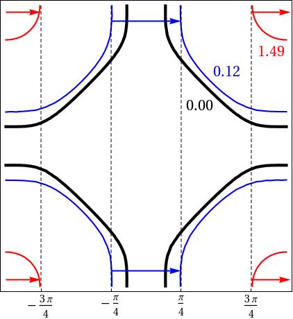
In this paper we present the first microscopic model of elastic RSXS in systems with charge order in the valence band, such as striped high-Tc cuprates [28, 29, 23, 30, 31, 32, 33, 34]. We develop a theoretical approach that allows us to analyze RSXS spectra in the case of itinerant valence electrons and include realistic bandstructures. Our formalism accounts for excitonic effects and the orthogonality catastrophe arising from the interaction of valence electrons with core holes (within the approximation of noninteracting valence electrons our analysis is exact) as well as the finite lifetime of core holes. We show that the two-peak spectrum observed in experiments at the O K edge of La1.875Ba0.125CuO4 [3, 9] can be explained by dynamical nesting of the “standard” band structure of cuprates (see Figs. 1 and 2). We find that interaction of valence electrons with the core hole changes the spectrum significantly. For a physically reasonable core hole potential we obtain quantitative agreement with the experimental data on underdoped La1.875Ba0.125CuO4 (LBCO) near the 1/8-anomaly [3] (similar spectra were observed for La1.8-xEu0.2SrxCuO4(LESCO) in [9]). Our results suggest that RSXS at the O K edge can be directly connected to the known band structure, providing a new, bulk-sensitive probe of electron quasiparticles that is complementary to ARPES and STM techniques.

Theoretical formalism for elastic RSXS.– Following Ref. [17] we consider an effective single band model describing resonant absorption and emission of photons
| (1) |
Here and are annihilation operators of electrons on site in the core orbital and valence band respectively, annihilates a photon with momentum and polarization , and are matrix elements whose precise form is not important to us. Resonant scattering is a second order process in
| (2) |
Here is the initial state of the system with electrons in the valence band, no core holes, and one incoming photon with momentum ; is the intermediate state with one core hole and one extra electron in the valence band, and no photons; is the final state with the core levels filled again, electrons in the valence band and one outgoing photon with momentum . We also introduced and to denote energies of the initial and intermediate electron states respectively. Note that the latter includes the potential of the core hole. is the decay rate of the core hole, including radiative and non-radiative processes. We focus on elastic scattering by ordering wavevector where we can take and .
Because the core hole is immobile it must be re-filled on the same site on which it is created and it may be subsumed into a static potential that acts on the valence electrons of the intermediate state. The core hole contributes the trivial matrix element . Therefore, Eq. (2) takes the following form:
| (3) | ||||
| (4) |
where and is the Hamiltonian of the valence electrons with and without the core hole potential. Here the matrix elements refer to the valence electron Fock space. When the core hole potential is zero, and reduces essentially to the retarded Green’s function[17]. If we measure photon frequencies relative to the difference between the chemical potential of the valence band and the energy of the core state electron , , we can set so that . The intermediate states are eigenstates of
| (5) |
where is the potential due to the core hole at site and is given in the grand canonical ensemble. Equation (4) also applies to thermal ensemble at temperature , provided that we use
| (6) |
The subscript on the trace denotes that it is taken with respect to Fock space.
Eqs. (4 - 6) are very general and apply for an arbitrary interacting valence band Hamiltonian . While Eq. (6) was formulated for the single band case, it can be generalized to the multi orbital case by adding orbital indices to electron operators and restoring orbital-dependent matrix elements for absorption and emission. In the remainder of this paper we will limit our discussion to the model of non-interacting electrons. This simplifying assumption is justified as long as the lifetime of electron states in the valence band is longer than the lifetime of the core hole (see also discussion below).
The trace in Eq. (6) is reminiscent of the orthogonality catastrophe of x-ray absorption [35, 36] and the Fermi edge singularity of mesoscopic transport [37, 38]. It expresses the many-body overlap of the initial Fermi sea with the perturbed Fermi sea that time evolves under and the single-particle dynamics of the extra electron injected into the valence band at site . It can be reduced to a product of determinants and inverse matrix elements of operators in single-particle Hilbert space [39, 40]. As an example, by appealing to a basis in which is diagonal, , the trace factors as . This in turn is the product of eigenvalues of the single-particle operator , hence it equals . Here refer to single particle operators for a single spin component of electrons. What permits further progress is that by the Baker-Campbell-Haussdorff Lemma can be written as where is quadratic, and hence the remaining traces can be evaluated in the same spirit [40]. We obtain 22 2 See Supplemental Material for derivation of trace formulae, variation of strength and form of the core hole potential, variation of hopping strength, and comments on slightly-inelastic scattering.
| (7) |
where is the occupation number operator and is the intermediate state time evolution operator. The determinantal factor corresponds to the many-particle dynamics of the Fermi sea. It is squared because the orthogonality catastrophe occurs for each of the two spin species regardless of the spin of the photo-excited electron ††footnotemark: . One can interpret it as follows: the argument is an operator that time-evolves only those states that are initially occupied, and taking the determinant computes an overlap of Slater states. The matrix element part corresponds to single-particle dynamics of the intermediate photoelectron. It is a local Green’s function for propagation of a single electron from site to site , modified by the Pauli-blocking term . For period- order, one needs to sum over inequivalent sites . The determinant can be evaluated efficiently for a finite system, converging by a system size of . Eqs. (4) and (7) constitute a convenient formula for calculating RSXS spectra in the approximation of noninteracting electrons. They treat exactly the interaction of electrons with the core hole and finite lifetime of the core hole.
RSXS of cuprates.– We apply Eqs. (4) and (7) to charge order in an effective one-band model of the cuprates
| (8) |
Eq. (8) is a mean-field phenomenological description of charge ordering [41, 42, 30, 43, 32, 44, 45, 46] that applies regardless of its microscopic origin. Possible mechanisms include electron-electron interactions, in which case charge order is often called stripes [34, 47], and nesting of the Fermi surface and electron-phonon interactions [48, 49, 50].
We use the tight-binding dispersion and parameters meV characteristic of LBCO [51]. For simplicity we ignore dispersion, which would at most smear energy peaks by an amount 50 meV [51]. Fig. 1 presents an RSXS spectrum for a contact core hole potential . We have also calculated spectra using Yukawa potentials of various ranges and found similar results ††footnotemark: . We have chosen a realistic core hole lifetime meV.
Two peak structure. Fig. 1 shows the calculated intensity of RSXS as a function of initial photon energy. The two peak structure of the spectrum agrees well with experimental findings [3, 9]. A simple physical argument shows that the two peak structure is a robust feature of the cuprate band structure. Consider the simplifying limit of zero core hole potential. In this case the intermediate eigenstates are obtained by adding an electron in some eigenstate of to the Fermi sea, and the energy domain expression Eq. (3) reduces to
| (9) |
Unoccupied states contribute strongly when their energy is in resonance and the Fourier transform of their density at wavevector is large. In the presence of a CDW potential, Bloch states and hybridize to form eigenstates with non-trivial density. This occurs most readily when are nearly degenerate. The RSXS intensity at energy comes from points on the surface of constant energy that are separated by wavevector [42]. Usually these are isolated pairs of points, but at certain energies the surfaces are nested so that sections separated by move in parallel (see Fig. 2). At these energies there is a large density of hybridized states. This is the phenomenon of dynamic nesting. While Fermi surface nesting, which is just dynamic nesting at , is uncommon, dynamic nesting is a generic consequence of symmetry. Consider the two-dimensional cuprate Brillouin zone and period-4 CDW wavevector . Any Bloch state on the lines and is degenerate with . Constant energy contours with segments tangent to the line also have segments tangent to ; these symmetry-equivalent segments are dynamically nested. Fermi surface nesting is not generic because there is no particular reason why the contour should be tangent to the lines (or, in three dimensions, a plane). Dynamic nesting, on the other hand, occurs when some energy contour is tangent to the lines. For our choice of LBCO hopping strengths the energy contours exhibiting dynamic nesting correspond to energies 0.1 eV and 1.5 eV above the Fermi level– which are separated by nearly the same amount as RSXS peaks. The small discrepancy is due to the tendency of the core hole potential to widen the distance between peaks and vanishes when we set ††footnotemark: .
A simplified model neglecting the core hole potential explains the spectrum and its two peaks qualitatively but does not give the correct relative weights of the two peaks ††footnotemark: . Including the core hole potential yields quantitative agreement with experiments. The core hole potential has a weak effect on the energy separation between the two peaks but dramatically decreases the intensity of the high-energy peak ††footnotemark: . A core hole potential strength meV, which is reasonable for a screened core hole interacting with valence electrons, reproduces the experimental ratios of peak intensities. A non-physical repulsive core hole decreases the intensity of the low-energy peak. The discussion of Ref. [17] connecting the RSXS spectrum to the electron spectral function thus remains largely accurate in the presence of a weak core hole potential. However, strong core hole potentials yield spectra with qualitative features, such as a lack of a high-energy peak, that give misleading conclusions in analyses based only on the spectral function. For example, we attribute the absence of a second peak in RSXS at the Cu L3/2 edge [3] to a strong Cu core hole potential. The spectrum is robust to changes in the core hole lifetime , which broadens the peaks, and the CDW strength , which scales the overall intensity. Small changes in the hopping strengths have little effect; multiplying them by a uniform factor affects the distance between peaks.
Our calculations provide the first quantitative explanation for the two peak structure observed in LBCO and LESCO [3, 9]. An earlier interpretation of the two peaks as arising from the lower and upper Hubbard bands, the so-called “spatially-modulated Mottness”, was not supported by quantitative analysis. Moreover, a separation of 1.9 eV between peaks is found in x-ray absorption spectroscopy (XAS) of LBCO and LSCO [52, 3]. According to the lower/upper Hubbard band interpretation, in which between peaks there is a gap, the separation between peaks in RSXS must be at least as large as the separation in XAS. Thus we think that dynamical nesting of the band structure provides a more natural interpretation of the two peak structure observed in LBCO and LESCO.
Discussion.– We now comment on the specific values of the band structure that we used in our analysis. Ab-initio LDA calculations on LSCO give meV [51] while fitting of the ARPES spectra gives [51]. The ratios among tight-binding parameters are nearly identical for both cases, so the band structure is well-known up to an overall truncation factor. The two peak character of the RSXS spectra appears for both band structures with nearly the same relative intensities of the two peaks. We find that taking either the LDA or ARPES dispersions gives peaks separated by 1.7 and 1.3 eV. We obtain the best fit to RSXS data by choosing parameters halfway between the two. We point out that it is not so surprising that band structure obtained from the ARPES data does not provide the best agreement with the RSXS spectra. ARPES data only exist within 200 meV of the Fermi surface [53], where the renormalization effect due to interactions is strongest, while we are interested in features at much higher energy. Additionally, it has been suggested that ARPES tends to underestimate electron dispersion relative to x-ray experiments [54, 51]. Another important issue is our approximation of non-interacting electrons. The key quantity entering our analysis is a generalized propagator (6). The effect of many-body correlations is to introduce decay of an electron into other excitations, but as far as the Green’s function is concerned this simply contributes an imaginary part to the electron’s self-energy (we assume that the effective one-band model we use has already incorporated renormalization via the real part of self-energies). Furthermore, if the decay of the electron is slow compared to the decay of the core hole, any broadening introduced by electron interactions will be hidden within the width . Conversely, if the electron decays very rapidly, RSXS peaks will be broadened into oblivion. Therefore, the presence of peaks in an RSXS spectrum puts an upper bound on the imaginary self-energy and implies that excitations resemble well-defined quasiparticles. We note that recent DMFT calculations 33 3 A. Georges, unpublished have found long-lived electron quasiparticles in the Hubbard model well above the Fermi energy, in contrast to short-lived hole-like excitations. RSXS, which probes high-energy electron excitations, complements ARPES, which probes hole-like excitations, and magnetic oscillation experiments [55, 56, 57], which probes only excitations near the Fermi energy.
Outlook.–The predictions of our model can be checked in future experiments. For example, recent work on charge order in underdoped YBCO [15], which was performed at energies corresponding to Cu L edges, could be repeated at the O K edge. We expect, as in LBCO, two peaks at energies determined by band structure. Also, systems with checkerboard charge order, with coexisting Fourier components and , will exhibit a harmonic at . If the latter harmonic is sufficiently strong, an RSXS signal will appear at this wavevector. One can see that this ordering wavevector also has dynamic nesting at two energies, so we expect to find a two peak spectrum44 4 D. Benjamin, unpublished.
Summary.– We have developed a microscopic model of RSXS that takes into account the itinerant character of valence electrons and excitonic effects. We showed that a simple physical picture of dynamical nesting found in the canonical band structure of cuprates gives rise to a two peak structure, while the core hole potential is necessary for quantitative agreement with the data. Our analysis shows that even at high energies electronic excitations behave like sufficiently well-defined quasiparticles described by the canonical band structure.
Acknowledgements.– We thank A. Georges and J. Sau for useful discussions. This work was supported by Harvard-MIT CUA, NSF Grant No. DMR-07-05472, and the ARO-MURI on Atomtronics (DB, DA, ED); and the U.S. Department of Energy grant DE-FG02-06ER46285 (PA).
References
- [1] P. Abbamonte, L. Venema, A. Rusydi, G. A. Sawatzky, G. Logvenov, and I. Bozovic, Science (New York, N.Y.) 297, 581 (2002), ISSN 1095-9203, URL http://www.sciencemag.org/content/297/5581/581.abstract.
- [2] S. Wilkins, P. Spencer, P. Hatton, S. Collins, M. Roper, D. Prabhakaran, and A. Boothroyd, Physical Review Letters 91 (2003), ISSN 0031-9007, URL http://prl.aps.org/abstract/PRL/v91/i16/e167205.
- [3] P. Abbamonte, A. Rusydi, S. Smadici, G. D. Gu, G. A. Sawatzky, and D. L. Feng, Nature Physics 1, 155 (2005), ISSN 1476-0000, URL http://dx.doi.org/10.1038/nphys178.
- [4] S. Dhesi, A. Mirone, C. De Nadaï, P. Ohresser, P. Bencok, N. Brookes, P. Reutler, A. Revcolevschi, A. Tagliaferri, O. Toulemonde, et al., Physical Review Letters 92 (2004), ISSN 0031-9007, URL http://prl.aps.org/abstract/PRL/v92/i5/e056403.
- [5] S. Grenier, J. Hill, D. Gibbs, K. Thomas, M. Zimmermann, C. Nelson, V. Kiryukhin, Y. Tokura, Y. Tomioka, D. Casa, et al., Physical Review B 69 (2004), ISSN 1098-0121, URL http://prb.aps.org/abstract/PRB/v69/i13/e134419.
- [6] P. Abbamonte, G. Blumberg, A. Rusydi, A. Gozar, P. G. Evans, T. Siegrist, L. Venema, H. Eisaki, E. D. Isaacs, and G. A. Sawatzky, Nature 431, 1078 (2004), ISSN 1476-4687, URL http://dx.doi.org/10.1038/nature02925.
- [7] I. Zegkinoglou, J. Strempfer, C. Nelson, J. Hill, J. Chakhalian, C. Bernhard, J. Lang, G. Srajer, H. Fukazawa, S. Nakatsuji, et al., Physical Review Letters 95 (2005), ISSN 0031-9007, URL http://prl.aps.org/abstract/PRL/v95/i13/e136401.
- [8] C. Schüß ler Langeheine, J. Schlappa, A. Tanaka, Z. Hu, C. Chang, E. Schierle, M. Benomar, H. Ott, E. Weschke, G. Kaindl, et al., Physical Review Letters 95 (2005), ISSN 0031-9007, URL http://prl.aps.org/abstract/PRL/v95/i15/e156402.
- [9] J. Fink, E. Schierle, E. Weschke, J. Geck, D. Hawthorn, V. Soltwisch, H. Wadati, H.-H. Wu, H. Dürr, N. Wizent, et al., Physical Review B 79 (2009), ISSN 1098-0121, URL http://prb.aps.org/abstract/PRB/v79/i10/e100502.
- [10] J. Herrero-Martín, J. García, G. Subías, J. Blasco, M. Sánchez, and S. Stanescu, Physical Review B 73 (2006), ISSN 1098-0121, URL http://prb.aps.org/abstract/PRB/v73/i22/e224407.
- [11] E. Nazarenko, J. E. Lorenzo, Y. Joly, J. L. Hodeau, D. Mannix, and C. Marin, Physical Review Letters 97 (2006), ISSN 0031-9007, URL http://prl.aps.org/abstract/PRL/v97/i5/e056403.
- [12] S. Smadici, P. Abbamonte, M. Taguchi, Y. Kohsaka, T. Sasagawa, M. Azuma, M. Takano, and H. Takagi, Physical Review B 75 (2007a), ISSN 1098-0121, URL http://prb.aps.org/abstract/PRB/v75/i7/e075104.
- [13] S. Smadici, P. Abbamonte, A. Bhattacharya, X. Zhai, B. Jiang, A. Rusydi, J. Eckstein, S. Bader, and J.-M. Zuo, Physical Review Letters 99 (2007b), ISSN 0031-9007, URL http://prl.aps.org/abstract/PRL/v99/i19/e196404.
- [14] S. Smadici, J. Lee, S. Wang, P. Abbamonte, G. Logvenov, A. Gozar, C. Cavellin, and I. Bozovic, Physical Review Letters 102 (2009), ISSN 0031-9007, URL http://prl.aps.org/abstract/PRL/v102/i10/e107004.
- [15] G. Ghiringhelli, M. L. Tacon, M. Minola, S. Blanco-Canosa, C. Mazzoli, N. B. Brookes, G. M. De Luca, A. Frano, D. G. Hawthorn, F. He, et al. (2012), eprint 1207.0915, URL http://arxiv.org/abs/1207.0915.
- [16] P. D. Hatton, S. B. Wilkins, T. A. W. Beale, T. K. Johal, D. Prabhakaran, and A. T. Boothroyd, Journal of synchrotron radiation 12, 434 (2005), ISSN 0909-0495, URL http://scripts.iucr.org/cgi-bin/paper?kv5008.
- [17] P. Abbamonte, E. Demler, J. C. S. Davis, and J.-C. Campuzano, p. 15 (2011), eprint 1112.5112, URL http://arxiv.org/abs/1112.5112.
- [18] M. Rohlfing and S. Louie, Physical Review Letters 80, 3320 (1998), ISSN 0031-9007, URL http://prl.aps.org/abstract/PRL/v80/i15/p3320_1.
- [19] A. Damascelli and Z.-X. Shen, Reviews of Modern Physics 75, 473 (2003), ISSN 0034-6861, URL http://rmp.aps.org/abstract/RMP/v75/i2/p473_1.
- [20] D. Lu, I. M. Vishik, M. Yi, Y. Chen, R. G. Moore, and Z.-X. Shen, Annual Review of Condensed Matter Physics 3, 129 (2012), ISSN 1947-5454, URL http://www.annualreviews.org/doi/abs/10.1146/annurev-conmatphys-020911-125027?prevSearch=ARPES&searchHistoryKey=.
- [21] M. Campuzano, J. C. and Norman, M. R. and Randeria, in Physics of Superconductors Vol. II, edited by J. Bennemann, K.H. and Ketterson (Springer, 2004), pp. 167–273.
- [22] O. Fischer, M. Kugler, I. Maggio-Aprile, C. Berthod, and C. Renner, Reviews of Modern Physics 79, 353 (2007), ISSN 0034-6861, URL http://rmp.aps.org/abstract/RMP/v79/i1/p353_1.
- [23] J. E. Hoffman, E. W. Hudson, K. M. Lang, V. Madhavan, H. Eisaki, S. Uchida, and J. C. Davis, Science (New York, N.Y.) 295, 466 (2002), ISSN 1095-9203, URL http://www.sciencemag.org/content/295/5554/466.abstract.
- [24] K. McElroy, D.-H. Lee, J. E. Hoffman, K. M. Lang, J. Lee, E. W. Hudson, H. Eisaki, S. Uchida, and J. C. Davis, Phys. Rev. Lett. 94, 197005 (2005), URL http://link.aps.org/doi/10.1103/PhysRevLett.94.197005.
- [25] M. Vershinin, S. Misra, S. Ono, Y. Abe, Y. Ando, and A. Yazdani, Science 303, 1995 (2004), URL http://www.sciencemag.org/content/303/5666/1995.abstract.
- [26] C. Howald, H. Eisaki, N. Kaneko, M. Greven, and A. Kapitulnik, Physical Review B 67 (2003), ISSN 1098-0121, URL http://prb.aps.org/abstract/PRB/v67/i1/e014533.
- [27] N.-C. Yeh and A. D. Beyer, International Journal of Modern Physics B (IJMPB) 23, 4543 (2009), URL http://www.worldscientific.com/doi/abs/10.1142/S021797920905403X.
- [28] J. M. Tranquada, B. J. Sternlieb, J. D. Axe, Y. Nakamura, and S. Uchida, Nature 375, 561 (1995), ISSN 0028-0836, URL http://dx.doi.org/10.1038/375561a0.
- [29] S. White and D. Scalapino, Physical Review B 61, 6320 (2000), ISSN 0163-1829, URL http://prb.aps.org/abstract/PRB/v61/i9/p6320_1.
- [30] S. A. Kivelson, I. P. Bindloss, V. Oganesyan, J. M. Tranquada, A. Kapitulnik, and C. Howald, Reviews of Modern Physics 75, 1201 (2003), ISSN 0034-6861, URL http://rmp.aps.org/abstract/RMP/v75/i4/p1201_1.
- [31] A. Millis and M. Norman, Physical Review B 76 (2007), ISSN 1098-0121, URL http://prb.aps.org/abstract/PRB/v76/i22/e220503.
- [32] M. Vojta, Advances in Physics 58, 699 (2009), ISSN 0001-8732, URL http://www.informaworld.com/openurl?genre=article&doi=10.1080/00018730903122242&magic=crossref||D404A21C5BB053405B1A640AFFD44AE3.
- [33] E. Berg, E. Fradkin, S. A. Kivelson, and J. M. Tranquada, New Journal of Physics 11, 115004 (2009), ISSN 1367-2630, URL http://stacks.iop.org/1367-2630/11/i=11/a=115004.
- [34] J. Zaanen and O. Gunnarsson, Physical Review B 40, 7391 (1989), ISSN 0163-1829, URL http://prb.aps.org/abstract/PRB/v40/i10/p7391_1.
- [35] G. Mahan, Physical Review 163, 612 (1967), ISSN 0031-899X, URL http://prola.aps.org/abstract/PR/v163/i3/p612_1.
- [36] P. Nozières and C. de Dominicis, Physical Review 178, 1097 (1969), ISSN 0031-899X, URL http://prola.aps.org/abstract/PR/v178/i3/p1097_1.
- [37] B. Muzykantskii, N. D’Ambrumenil, and B. Braunecker, Physical Review Letters 91 (2003), ISSN 0031-9007, URL http://prl.aps.org/abstract/PRL/v91/i26/e266602.
- [38] D. Abanin and L. Levitov, Physical Review Letters 94 (2005), ISSN 0031-9007, URL http://prl.aps.org/abstract/PRL/v94/i18/e186803.
- [39] M. Combescot and P. Nozières, Journal de Physique 32, 913 (1971), URL http://jphys.journaldephysique.org/index.php?option=com_article&access=doi&doi=10.1051/jphys:019710032011-12091300&Itemid=129.
- [40] I. Klich, in Quantum Noise in Mesoscopic Physics, edited by Y. Nazarov (Springer, 2003), URL http://www.springer.com/physics/quantum+physics/book/978-1-4020-1239-6.
- [41] G. Grüner, Density Waves in Solids (Addison-Wesley, 1994).
- [42] D. Podolsky, E. Demler, K. Damle, and B. Halperin, Physical Review B 67 (2003), ISSN 0163-1829, URL http://prb.aps.org/abstract/PRB/v67/i9/e094514.
- [43] A. Hackl, M. Vojta, and S. Sachdev, Physical Review B 81 (2010), ISSN 1098-0121, URL http://prb.aps.org/abstract/PRB/v81/i4/e045102.
- [44] T. A. Sedrakyan and A. V. Chubukov, Physical Review B 81 (2010), ISSN 1098-0121, URL http://prb.aps.org/abstract/PRB/v81/i17/e174536.
- [45] H. Yao, D.-H. Lee, and S. Kivelson, Physical Review B 84 (2011), ISSN 1098-0121, URL http://prb.aps.org/abstract/PRB/v84/i1/e012507.
- [46] I. Martin, G. Ortiz, A. V. Balatsky, and A. R. Bishop, International Journal of Modern Physics B 14, 3567 (2000), eprint http://www.worldscientific.com/doi/pdf/10.1142/S0217979200003630, URL http://www.worldscientific.com/doi/abs/10.1142/S0217979200003630.
- [47] H. Schulz, Physical Review Letters 64, 1445 (1990), ISSN 0031-9007, URL http://prl.aps.org/abstract/PRL/v64/i12/p1445_1.
- [48] J.-X. Li, C.-Q. Wu, and D.-H. Lee, Physical Review B 74 (2006), ISSN 1098-0121, URL http://prb.aps.org/abstract/PRB/v74/i18/e184515.
- [49] K. M. Shen, F. Ronning, D. H. Lu, F. Baumberger, N. J. C. Ingle, W. S. Lee, W. Meevasana, Y. Kohsaka, M. Azuma, M. Takano, et al., Science (New York, N.Y.) 307, 901 (2005), ISSN 1095-9203, URL http://www.sciencemag.org/content/307/5711/901.abstract.
- [50] O. Andersen, A. Liechtenstein, O. Rodriguez, I. Mazin, O. Jepsen, V. Antropov, O. Gunnarsson, and S. Gopalan, Physica C: Superconductivity 185-189, 147 (1991), ISSN 09214534, URL http://dx.doi.org/10.1016/0921-4534(91)91964-6.
- [51] R. S. Markiewicz, S. Sahrakorpi, M. Lindroos, H. Lin, and A. Bansil, Physical Review B 72 (2005), ISSN 1098-0121, URL http://prb.aps.org/abstract/PRB/v72/i5/e054519.
- [52] D. C. Peets, D. G. Hawthorn, K. M. Shen, Y.-J. Kim, D. S. Ellis, H. Zhang, S. Komiya, Y. Ando, G. A. Sawatzky, R. Liang, et al., Physical Review Letters 103 (2009), ISSN 0031-9007, URL http://prl.aps.org/abstract/PRL/v103/i8/e087402.
- [53] A. Ino, C. Kim, M. Nakamura, T. Yoshida, T. Mizokawa, A. Fujimori, Z.-X. Shen, T. Kakeshita, H. Eisaki, and S. Uchida, Physical Review B 65 (2002), ISSN 0163-1829, URL http://prb.aps.org/abstract/PRB/v65/i9/e094504.
- [54] S. Hüfner, Photoelectron Spectroscopy: Principles and Applications (Springer, 2003).
- [55] D. LeBoeuf, N. Doiron-Leyraud, J. Levallois, R. Daou, J.-B. Bonnemaison, N. E. Hussey, L. Balicas, B. J. Ramshaw, R. Liang, D. A. Bonn, et al., Nature 450, 533 (2007), ISSN 1476-4687, URL http://dx.doi.org/10.1038/nature06332.
- [56] N. Doiron-Leyraud, C. Proust, D. LeBoeuf, J. Levallois, J.-B. Bonnemaison, R. Liang, D. A. Bonn, W. N. Hardy, and L. Taillefer, Nature 447, 565 (2007), ISSN 1476-4687, URL http://dx.doi.org/10.1038/nature05872.
- [57] B. Vignolle, D. Vignolles, D. LeBoeuf, S. Lepault, B. Ramshaw, R. Liang, D. Bonn, W. Hardy, N. Doiron-Leyraud, A. Carrington, et al., Comptes Rendus Physique 12, 446 (2011), ISSN 16310705, URL http://dx.doi.org/10.1016/j.crhy.2011.04.011.