Screened hybrid functional applied to 33 transition-metal perovskites LaO3 (=Sc-Cu): influence of the exchange mixing parameter on the structural, electronic and magnetic properties
Abstract
We assess the performance of the Heyd-Scuseria-Ernzerhof (HSE) screened hybrid density functional scheme applied to the perovskite family LaO3 (=Sc-Cu) and discuss the role of the mixing parameter (which determines the fraction of exact Hartree-Fock exchange included in the density functional theory (DFT) exchange-correlation functional) on the structural, electronic, and magnetic properties. The physical complexity of this class of compounds, manifested by the largely varying electronic characters (band/Mott-Hubbard/charge-transfer insulators and metals), magnetic orderings, structural distortions (cooperative Jahn-Teller like instabilities), as well as by the strong competition between localization/delocalization effects associated with the gradual filling of the and orbitals, symbolize a critical and challenging case for theory. Our results indicates that HSE is able to provide a consistent picture of the complex physical scenario encountered across the LaO3 series and significantly improve the standard DFT description. The only exceptions are the correlated paramagnetic metals LaNiO3 and LaCuO3, which are found to be treated better within DFT. By fitting the ground state properties with respect to we have constructed a set of ’optimum’ values of from LaScO3 to LaCuO3: it is found that the ’optimum’ mixing parameter decreases with increasing filling of the manifold (LaScO3: 0.25; LaTiO3 & LaVO3: 0.10-0.15; LaCrO3, LaMnO3, and LaFeO3: 0.15; LaCoO3: 0.05; LaNiO3 & LaCuO3: 0). This trend can be nicely correlated with the modulation of the screening and dielectric properties across the LaO3 series, thus providing a physical justification to the empirical fitting procedure. Finally, we show that by using this set of optimum mixing parameter HSE predict dielectric constants in very good agreement with the experimental ones.
pacs
71.27.+a, 71.15.-m, 71.10.-w, 71.28.+d, 71.20.Be, 78.30.Er, 75.25.-jI INTRODUCTION
The physics of transition metal perovskites with general chemical formula ABO3 (where A is a large cation, similar in size to O2- and B is a small transition metal (TM) cation) has attracted and challenged the interest and curiosity of the material science community for many decades, due to huge variety of complex phenomena arising from the subtle coupling between structural, electronic and magnetic degrees of freedom. The high degree of chemical flexibility and the localized (i.e. not spatially homogeneous) character of the dominant TM partially filled states lead to the coexistence of several physical interactions – spin, charge, lattice and orbital – which are all simultaneously active. The occurrence of strong lattice-electron, electron-spin and spin-orbit couplings causes several fascinating phenomena, including metal-insulator transitions[1, 2], superconductivity[3], colossal magnetoresistance[4, 5], multiferroicity[6], bandgaps spanning the visible and ultraviolet[7], and surface chemical reactivity from active to inert[8, 9]. When the additional degrees of freedom afforded by the combinatorial assemblage of perovskite building blocks in superlattices, heterointerfaces and thin films are introduced the range of properties increases all the more, as demonstrated by the recent several remarkable discoveries in the field of oxide heterostructures[10]. Tunability and control of these intermingled effects can be further achieved by means of external stimuli such as doping[11, 12], pressure[13, 14], temperature and magnetic or electric fields[15, 16], thereby enhancing the tailoring capability of perovskites for a wide range of functionalities. This rich array of behaviors uniquely suit perovskites for novel solutions in different sectors of modern technology (optoelectronics, spintronics, piezoelectric devices and (photo)catalysis), for which conventional semiconductors cannot be used[17, 18, 19, 20].
Theoretical studies of TM perovskites, aiming to describe and understand the underlying physical mechanisms determining their complex electronic structures have been mainly developed within two historically distinct solid state communities, model Hamiltonians[21, 22] and first principles[23], which in the recent years have initiated to fruitfully cross-connect each other methodologies towards more general schemes such as DFT+DMFT (Density Functional Theory[24] + Dynamical Mean Field Theory[25, 26, 27]), with the aim to overtake the individual limitations and to improve the applicability and predictive power of electronic structure theory[28, 29]. Model Hamiltonians approaches adopt simplified lattice fermion models, typically the celebrated Hubbard model, inspired by the seminal works of Anderson[30], Hubbard[31] and Kanamori[32] in which the many-body problem is solved using a small number of relevant bands and short-ranged electron interactions. These effective models can solve the many-body problem very accurately, also including ordering and quantum fluctuations, but critically depends on an large number of adjustable parameters (which can be in principle derivable by first principles schemes[33, 35, 38, 39, 40, 41]), and its applicability is restricted to finite-size systems[2, 29]. In DFT the intractable many-body problem of interacting electrons is mapped into a simplified problem of non-interacting electrons moving in an effective potential throughout the Kohn-Sahm scheme[24], and electron exchange-correlation (XC) effects are accounted by the XC potential which is approximated using XC functionals such as the Local Density Approximation (LDA), the Generalized Gradient Approximation (GGA) et similaria[42]. As the name suggests, in DFT the ground state properties are obtained only from the charge density, and this makes DFT fundamentally different from wavefunction-based approaches as the Hartee-Fock method, the simplest approximation to the many-body problem which includes the exact exchange but no correlation[43]. Though DFT has been widely and successfully used in the last 40 years in solid-state physics and quantum-chemistry to calculate structural data, energetics and, to a lesser extent, electronic and magnetic properties, it suffers of fundamental difficulties mostly due to the approximate treatment of XC effects. This drawback is particularly severe when DFT is applied to the so called strongly correlated systems (SCSs), whose prototypical examples are transition metal oxides (TMOs). A systematic improvement of these XC-related deficiencies in DFT is essentially impossible, but several ’beyond-DFT’ approaches have been proposed which deliver much more satisfying results. The most renewed ones are the DFT+U[44], SIC[45, 46, 47, 48], hybrid functionals[49], and GW[50]. For a recent review on DFT and beyond applied to transition metal oxides see 51.
| LaScO3 | LaTiO3 | LaVO3 | LaCrO3 | LaMnO3 | LaFeO3 | LaCoO3 | LaNiO3 | LaCuO3 | |
|---|---|---|---|---|---|---|---|---|---|
| Crystal structure | O- | O- | M- | O- | O- | O- | R- | R- | T-P4/m |
| TM electronic configuration | |||||||||
| 3+ | 3+ | 3+ | 3+ | 3+ | 3+ | 3+ | 3+ | 3+ | |
| Electronic character | I | I | I | I | I | I | I | M | M |
| Magnetic structure | NM | G-AFM | C-AFM | G-AFM | A-AFM | G-AFM | PM | PM | PM |
In this article we applied the screened hybrid functional introduced by Heyd, Scuseria, and Ernzerhof (HSE) [52] to study the structural, electronic and magnetic properties of the series of 3 TMO perovskites LaO3, with ranging from Sc to Cu. This is a rather challenging family of compounds for electronic structure methods for several reasons[53, 54, 55, 56, 57, 58, 60, 61, 62, 59, 63, 64, 65, 66, 67, 68, 69, 70, 71, 72, 73, 74, 75, 76, 77, 78, 79, 80, 81, 82, 83, 84, 85, 86, 87, 88, 41, 89] (see Table 1: (i) it encompasses band, Mott-Hubbard (MH) and charge-transfer (CT) insulators as well as correlated metals (the last two members of the series: LaNiO3 and LaCuO3)[7]; (ii) different type of antiferromagnetic (AFM) orderings are encountered across the series (A-type, C-type and G-type, graphically represented in Fig.1), but also non-magnetic (NM, LaScO3) and paramagnetic (PM, La(CoCu)O3 systems[55]; (iii) the dominating electronic character varies from to , and ranges from / localization (with variable crystal filed splitting between and states) to more spatially delocalized -orbitals[55]; (iv) the crystal symmetry spans orthorhombic (O), monoclinic (M), rhombohedral (R) and tetragonal (sketches of the crystal structures is given in Fig.2) characterized by a different level of structural distortions (Jahn-Teller (JT: staggered disproportionation of the -O bondlengths), GdFeO3-type (GFO: collective tiltings and rotations of the oxygen octahedra), monoclinic angle ).


Before describing the method and presenting the result we briefly recall previous ab initio investigations of this set of compounds performed using conventional DFT and ”beyond-DFT” methodologies. The most widely studied member of this family is certainly the classical JT-GFO distorted Mutt-Hubbard AFM insulator LaMnO3, but also other compounds have received significant attention, in particular LaTiO3 and LaVO3, and to a lesser extent, LaFeO3, LaCoO3, LaNiO3, and LaCuO3. Relatively scarce studies on the band insulator LaScO3 are present in literature.
DFT[53, 55, 56, 60, 61, 62, 63, 68, 75, 83, 86, 41, 89]: The seminal works of the Terakura group in the late 90s[55, 56, 60, 61, 62] have extensively assess the performance of LDA for the LaO3 series (=Ti-Cu), and revealed that LDA is unable to predict the observed insulating ground state for the first members (LaTiO3 and LaVO3), wrongly favors a non magnetic solution for LaTiO3 and severely underestimate the insulating gap in LaCrO3, LaMnO3, LaFeO3, and LaCoO3. The situation does not improve using the GGA[62]. However, the recent GGA-based re-exploration of the electronic properties of LaCrO3 by Ong et al.[75] has reported that a good agreement with experiment can be achieved, upon a proper (re)interpretation of the optical spectra. It should be noticed that all these results were obtained using the experimental geometries. The very few structural optimizations at DFT level, mostly focused on LaMnO3, have shown that though LDA/GGA reproduce the experimental volume within 1-3 % [83, 71, 89], the lattice distortions associated with the JT and GFO instabilities are significantly underestimated. For compounds with more delocalized 3 electrons like LaNiO3 the LDA performance get better as recently reported by Guo et al.[86].
DFT+U[53, 55, 58, 61, 62, 59, 65, 66, 69, 70, 71, 73, 74, 75, 77, 78, 79, 80, 81, 83, 84, 91, 85, 86, 41]: In some cases the drawbacks of LDA and GGA in treating localized partially filled states can be adjusted by introducing a strong Hartree-Fock like intra-atomic interaction U properly balanced by the so-called double-counting (dc) correction. The resulting LDA(GGA)+U energy functional can be written as[44]
| (1) |
where is the operator for the number of electrons occupying a particular site and is its expectation value. This expression can be written in terms of the direct (U) and exchange (J) contributions, which lead to a set of slightly different LDA(GGA)+U energy functionals depending on the way the dc term is constructed[92]. Among the numerous applications of DFT+U to LaO3 the study of I. Solovyev and coworkers represents the most comprehensive and systematic one[55]. There it is found that LDA+U conveys a substantially improved description of the bandstructure of LaO3 from LaTiO3 to LaCuO3 with respect to conventional DFT, though the results critically depend on the specific treatment of localization effects in the 3 manifold. By applying U-correction to electrons only the authors show that LaTiO3 and LaVO3 are correctly predicted to be insulating, thus curing the deficient LDA picture. At variance with DFT LaTiO3 is found to be magnetic, but with a magnetic moment twice larger than the experimental one. The bandgap of early (LaTiO3, LaVO3) and late (LaCoO3) LaO3 members which have a predominant character are better described than the compounds LaMnO3 and LaFeO3, for which an on site U applied to the entire 3 is needed to improve the agreement with experiment. The values of the gap clearly depends on the value of the U parameter, as discussed by Z. Yang et al.[59]. By fitting the U using the measured gap as reference quantity, these authors have shown that the best agreement with experiment is achieved for U progressively increasing from 5 eV (LaCrO3) to 7 eV (LaNiO3), about 2 eV smaller than those computed by I. Solovyev using constrained LDA[55]. Similarly to the standard LDA case, few attempts have been made to optimize the structural parameters at DFT+U level[61, 74, 83, 84, 86]: (i) LaTiO3. H.S. Ahn[74] and coworkers have shown that the application of LDA+U (U=3.2 eV) systematically increase the (underestimated) LDA lattice parameters of LaTiO3 and the internal distortions, thus improving the overall agreement with experiment. (ii) LaMnO3. using the Perdew-Burke-Ernzerhof[93] (PBE) approximation with an on-site effective U=2 eV T. Hashimoto et al.[83] have performed a full (volume and internal coordinates) structural optimization in LaMnO3 and demonstrated that, unlike GGA, GGA+U accounts well for the experimental JT and tilting distortions; (iii) LaCoO3. H. Hsu et al.[77] and A. Laref et al.[84] have shown that LDA+U describes well the lattice parameter, rhombohedral angle and atomic coordinates of LaCoO3; better agreement with experiment is obtained using a self-consistent U[77] rather than a fixed U value of 7-8 eV[84]. (iv) LaNiO3. The work of G. Guo et al.[86] on LaNiO3 reported that for this correlated metal LDA+U (U=6 eV) delivers geometrical data very similar to the already satisfactory LDA ones (though, as already pointed out, LDA does a better job in predicting the electronic properties).
HF[57, 72, 94]: The application of a purely Hartee-Fock (HF) procedure, i.e. including an exact treatment of the exchange interaction and neglecting electron correlation, has been extensively investigated by T. Mizokawa and A. Fujimori[57] and by I. Solovyev[72]. Though the HF method suffers for the absence of electron correlation which is reflected by its tendency to overestimate the magnitude of band gaps (which can be cured by including the correlation effects beyond the HF approximation), these studies show that HF can qualitatively explain the ground state electronic and magnetic properties of this class of magnetic oxides. Important exceptions are LaNiO3 and LaCuO3, which are found to be FM insulator (LaNiO3) and G-type AFM insulator (LaCuO3), in contrast with the observed PM metallic ground state. Another critical case for HF and in general for electronic structure methods is the origin of the type-G AFM ordering in LaTiO3[57, 95, 96, 72]: in Ref.57 the authors report that the stabilization of the G-type arrangement can be achieved by fixing the angle to approximately the experimental value. The resulting magnetic moment, downsized by spin orbit interaction effect, results in good agreement with the measured value, but the calculated bandgap is dramatically wrong, about 2.7 eV, against the measured value of 0.1 eV[7]. The results of Ref.72 go to the opposite direction: the magnetic ground state remains wrong even upon inclusion of correlation effects, but the bandgap, 0.6 eV, is in much better agreement with experiment. A similar trend is also observed for LaVO3.
Hybrid Functionals[64, 67, 82, 86, 87, 88, 41, 89, 97, 98, 99]: An alternative methodology to DFT and HF which has attracted a considerable attention in the solid state physics and chemistry communities in the last two decades is the so called hybrid functional approach. Originally introduced by A.D.J. Becke in 1993[49], the hybrid functional scheme relays on a suitable mixing between HF and (LDA/GGA) DFT theories, in which a portion of the exact HF exchange
| (2) |
is mixed with the complementary LDA/GGA approximated exchange . The resulting general hybrid XC kernel (decomposed over its exchange (X) and correlation (C) terms) can be written in the form:
| (3) |
where the mixing factor controls the amount of exact incorporated in the hybrid functional. Similarly to DFT+U (which makes use of the HF-like intra-atomic interaction U, as recalled above) hybrid functionals tends to correct the LDA/GGA delocalization error and to provide a better description of TMO with partially filled and states. The advantages with respect to DFT+U is that hybrid functionals (i) do not suffer from the double counting term (see Eq. 1) and, even most importantly, (ii) use an orbital dependent functional acting on all states, extended as well as localized (in the DFT+U method, the improved treatment of exchange effects is limited to states localized inside the atomic spheres, and usually limited to the partially filled TM shell). Though both schemes problematically depends on parameters such as U and J in DFT+U and the mixing factor in hybrid functionals, many attempts have been made to overcome these difficulties[100, 101, 102, 103, 104, 105, 106].
Though sparse in literature, hybrid functionals studies of LaO3 are increasing in the last few years [64, 67, 107, 82, 86, 87, 108, 41, 89, 109]. Applications of the renowned Becke, 3-parameter, Lee-Yang-Parr B3LYP functional[49] to LaMnO3[64, 67, 87] have shown that this method properly favors the type-A AFM ground state and provides an accurate description of the band gap, magnetic coupling constants, and Gibbs formation energies. The only structural optimization of the JT-distorted structure, however, deliver lattices constants which deviate by 5% from experiment[87]. We have recently reported that HSE performs very well in predicting the ground state properties of LaMnO3, including the optimized structural parameters, and that the data are slightly dependent on the actual value of the mixing factor[41, 89]. D. Gryaznov et al. have successfully studied the structural and phonon properties of LaCoO3 using the PBE0 (Perdew-Ernzerhof-Burke)[110] hybrid functional and reported a substantial improvement with respect to conventional DFT. The application of HSE and PBE0 functionals to LaNiO3, conversely, turned out to give poor agreement with the experimental photoemission spectroscopy (PES); this is in line with precedent unsatisfactory HSE/PBE0 results obtained for other itinerant magnetic metals[111]. The influence of the non-local exchange on the electronic properties of LaTiO3 has been investigated recently by F. Iori and coworkers[109]. By adopting the experimental structure these authors clarified that the improved description of HSE over DFT+U is due to a correct re-positioning of the O states, and show that by fixing the mixing parameter to its ”standard” value, 0.25, the bandgap and the magnetic moment are significantly overestimated with respect to measurements.
SIC[113, 112]: Another approach to correct the self-interaction (SI) LDA/GGA problem is the self-interaction correction method[45, 46, 47, 48], in which an approximated (atomic-like and orbitally averaged) self-interaction is subtracted from the LDA XC functional. Though conceptually different from LDA+U (in LDA+U an additional effective Coulomb term is added to the LDA/GGA functional), the SIC method is often pragmatically viewed as a generalized LDA+U approach in which the atomic SI plays the role of the U[112]. Several implementations of the SIC scheme have been proposed, characterized by a different level of complexity in treating the SI term and from the different underlying computational framework[45, 46, 47, 48], but all demonstrated an appreciable accuracy in predicting and interpreting the electronic structure of a vast range of systems, including SCSs and TMOs[114].
A valid illustration of the performance of the SIC method is supplied by the results obtained for LaTiO3 recently discussed by Filippetti et al.[112]. By assuming the experimental cell parameters SIC finds the correct AFM type-G insulating ordering and delivers internal structural distortions close to the experimental ones. As a downside, however, the magnitudes of the bandgap (1.6 eV) and magnetic moment (0.89 ) are substantially larger than the corresponding measured values (0.2 eV and 0.5 , respectively). Other SIC applications to the LaO3 series are limited, to our knowledge, to the ideal undistorted cubic phase of LaMnO3[113], for which a stringent comparison with experiment is difficult to do.
GW[76, 78, 41]: We finally recall the main achievements on LaO3 acquired using the GW approximation, a computational method fundamentally different from both DFT and HF. GW is configured to reflect and to treat the quasi-particle nature of electrons on the basis of Green’s function many-body perturbation theory[50], by explicitly accounting for the non-local and frequency-dependent self-energy () in a suitably rewritten Schrödinger-like equation. In the GW approximation is approximated to the lowest order term of the Hedin’s equation, and can be written as:
| (4) |
where G is the Green’s function and W is the dynamically screened Coulomb kernel. In the most widely used single-shot G0W0 approximation both G and W are treated in an unperturbed manner, but with increasing computer power self-consistent or partially self-consistent GW schemes are becoming more and more possible[115, 116, 41]. Due to the extensive computing time required to perform GW-like calculations, only few GW data are available in literature for complex systems. Among these, the works of Y. Nohara et al.[76, 78] represent a very comprehensive example of a systematic application of GW to LaO3 starting from preconvergent LDA+U wavefunctions. These authors have obtained excellent agreement with experimental spectra, but probably due to the uncertainties connected to the choice of U in preparing the initial wavefuncitons the values of the computed bandgaps deviate significantly from the experimental estimations, especially for LaTiO3, LaVO3, and LaCoO3. Good agreement with experiment has been also obtained for LaMnO3 using a partially self-consistent GW0 approach, in this case starting from GGA wavefunction[41].
The paper is organized as it follows. In Section II we illustrate the computational method and its technical aspects; in Section III we report the results on the structural optimization (Section III.1) and electronic & magnetic properties (Section III.2). A more general discussion on the observed trends and behaviors is developed in Section IV, and finally in Section V we draw our summary and conclusions.
II COMPUTATIONAL ASPECTS
All calculations were performed using the Vienna ab initio Simulation Package (VASP)[117, 118] employing DFT and hybrid-DFT approaches within the projector augmented wave method[119, 120] and the PBE parametrization scheme[93] for the XC functional. In the screened hybrid-DFT HSE approach adopted in this study, part of the short-range (sr) PBE exchange functional is replaced by an equal portion of exact HF exchange, according to the general prescription:
| (5) |
where , controls the range separation between the sr and long-range (lr) part of the Coulomb kernel (1/, with ), decomposed over long (L) and short (S) terms:
| (6) |
The reason to include a screening parameter is motivated by the computational effort required in computing the spatial decay of the HF X interaction. In the refined HSE06 hybrid functional, is set equal to 0.20 which corresponds to the distance 2/ at which the HF X interactions starts to become negligible. For =0 the PBE0 functional is recovered[110], whereas for HSE becomes identical to PBE. Beside the computational cost, the main beneficial consequence of the inclusion of a screening strategy in PBE0 is that screened hybrids can give access to the metallic state, which is unaffordable by unscreened PBE0-like hybrids. The HSE method has proven to to improve the quantitative and qualitative prediction of a large variety of materials, incluiding conventional semiconductors[121, 122], transition metal oxides[123, 124, 125], ferroeletrics[126], and surfaces[127, 128]. The mixing parameter , determining the amount of exact non-local HF X included in the hybrid XC functional is usually set to 0.25[52]. In this HSE case the PBE functional is recovered for =0.
Thus, the HSE06 depends by construction on two parameters, and . Though their standard values are routinely used in solid state calculations, it is to be expected that they may vary from material to material[106, 129], or that they may be property-dependent[130, 131, 64]. Unfortunately, a rigorous first principle procedure to determine the choice of these parameters does not exist. The conventional value =1/4 is determined by perturbation theory[110]. The choice has proven to be a practical compromise between computational cost and quality of the results[132]. Considering that most of the tests and fitting procedures have been performed taking as a reference atomic or molecular energetical and structural properties, the direct acquisition of these standard values in extended solid state system is not straightforward[110, 132].
By linking hybrid density functional theory with many-electron XC self-energy within a GW framework it has been proposed that the mixing factor can be interpreted as the inverse of the dielectric constant [133, 134, 135, 129]. Based on this idea, an approximated recipe to determine the optimum value of can be obtained:
| (7) |
which depends solely on the dielectric constant and on the ”unknown” factor of proportionality. It is important to emphasize that this relation should be interpreted as an a posteriori justification of the choice of the optimum value of , and not as a fundamental quantum mechanical definition of the mixing factor. It follows straightforwardly that for metal () is equal to zero. Several limitations affect this practical rule and degrade its ab initio nature[135], above all an accurate calculation of the dielectric constant, which is presently very difficult in particular for complex TMOs.
Following this line of thought other strategies have been introduced to overcome this problem invoking density-functional estimators[136] in the spirit of the Tran and Blaha functional[137], which furnishes parametric expressions inevitably dependent on the specific material dataset, usually limited to monoatomic and binary semiconductors[106]. To complicate the situation even further, there is some amount of arbitrariness in transferring the relation from unscreened PBE0-like hybrids to screened ones like HSE, where screening is already present in some form in the range separation controlled by the screening factor . These complications become particularly cumbersome when one moves from ’standard’ monoatomic and binary semiconductors to the more complex ternary TM perovskites. As a matter of fact, due to the absence of a systematic study on the influence of in this class of compounds, the large majority of hybrid functionals studies on ternary TMOs have been performed using the standard 1/4 compromise, though there are neither fundamental nor practical justifications for this choice.
Thus, in order to shed some light on the role of in a representative class of ternary TMOs with a largely varying degree of screening and competition between localization/delocalization effects we have performed our HSE calculations using 4 different values of : (i) low mixing (strong screening): 0.10 (HSE-10), 0.15 (HSE-15), (ii) standard mixing: 0.25 (HSE-25), and (iii) high mixing (low screening): 0.35 (HSE-35). The careful analysis of structural, electronic and magnetic properties will allow us to draw some general trends which should serve as a guidance for future HSE applications.
Technical setup: The plane wave cutoff energy was set to 300 eV. A 444, 666, 888 Monkhorst-Pack -points grids were used to sample the Brillouin zones for Pnma/P, R, and P4/m structures, respectively. Structural optimization was achieved by relaxing the volume, lattice parameters, lattice angles and internal atomic positions throughout the minimization of the stress tensor and forces using standard convergence criteria. Finally, the dielectric constant were computed adopting the perturbation expansion after discretization (PEAD) method[138, 116].
III RESULTS
This section is subdivided into two parts which are devoted to the presentation of the structural (Sec. III.1), and electronic and magnetic (Sec. III.2) properties, respectively. In each subsection we will summarize the specific results obtained for each member of the LaO3 series, and in the next section (Sec. IV) we will provide a more reasoned discussion on the general trends observed across the series.
As anticipated in the introduction hybrid functionals can be simplistically viewed as an orbital-dependent DFT+U approach in which the on-site electron-electron interaction parameter U is replaced by the parametric inclusion of a portion of the exact HF exchange quantified by the mixing factor . In DFT+U calculations, the U is usually either tuned to fit some specific physical property (i.e. bandgap, magnetic moment, volume, etc.), or calculated within constrained-LDA procedures[100, 101, 102, 103, 104]. In contrast, most of the available HSE-based calculations present in literature are done at fixed mixing parameter =0.25. This might erroneously convey the idea of a minor role played by the mixing factor or, even more fundamentally misleading, that HSE is a purely ab initio (i.e. parameter free) scheme. As already discussed previously, in the last few years the modeling community has started to address this issue[64, 106, 129] but the amount of available data are still very limited, in particular for complex oxide. It is therefore instructive to briefly recall a few results on the choice of the U in DFT+U studies of transition metal oxides in order to possibly formulate some expectations on the behavior of the mixing parameter in HSE. A good example to start with are transition metal monoxides (TMOs: MnO, FeO, CoO and NiO), where the TM possesses the oxidation state 2+ (). Several LDA+U studies have shown that a U between 6 and 8 eV can provide an accurate enough prediction of band gaps for all TMOs[139, 44]. Going from to the number of the localized electrons decreases. Thus, it might be expected that the magnitude of the Coulomb interaction increases due to the contraction of the spatial extension of the of the 3 () wave functions.[140] However, by comparing O and LaO3 photoemission data it can be unambiguously concluded that the effective Coulomb interaction decreases in compounds[140, 142, 143, 144, 141, 145].
Under the assumption that in LaO3 the electrons are localized and the electrons are itinerant, Solovyev[55] has explained this apparent contradiction by invoking the strong screening associated with the electrons. Indeed, the computed value of U for the shell in LaO3 are significantly reduced with respect to U for the states in O. The strength of the screening depends on the filling of the orbital: it is strong at half-filling and less efficient when the are nearly empty of occupied. The results of Solovyev indicate that this -U approach reproduces sufficiently well the main features of early (Ti-V-Cr) and late (Co-Ni) LaO3 compounds but fails for LaFeO3 (much too small bandgap and magnetic moment) and LaMnO3 (small gap). Clearly, effects other than itinerancy contribute to the strength of the U, such as the screening from non-3 electrons, (3/4)-O(2) hybridization, and lattice relaxation which can explain the discrepancy between self-consistent +U methods and experiments.
A fitting-U approach can selectively adjust the comparison with the experimental gap (not for LaCrO3) at the expense of a rigorous description of the position of the , and O() sub-bands (i.e. the ’correct’ value of the bandgap can arise from an fundamentally incorrect artificial electronic structure). This failure prevents any physically sound specification/understanding of the (MH or CT) character of the gap: in Ref.59, for instance, the gap of LaMnO3 is found to be predominantly CT like, in discrepancy with the actual situation (LaMnO3 is a MH insulator with a gap opened between occupied and empty states, partially hybridized with O states). Furthermore, the ’optimum’ U’s resulting from fitting-U schemes do not seem to reflect the observed to U-reduction, which is an additional sign of the inadequacy of such a procedure.
Considering that standard HSE (=0.25) performs quite well for TM monoxides[146, 123] we can expect that a smaller value will turn out to be more appropriate for reproducing the ground state properties of LaO3. Furthermore, given the full-orbital character of HSE we may expect that hybridization effects and screening from non 3 electrons will be better described as compared to DFT+U. Finally, we should point out that the choice to perform a complete structural optimization at each considered value of allows for a more genuine account of the structural contribution to the screening which is disguised in frozen lattice (atomic positions fixed to experimental ones) calculations.
III.1 Structural Properties
As already mentioned in the introduction four different crystal symmetries are encountered across the LaO3 series (see Fig. 2): (i) Orthorhombic Pnma for LaScO3, LaTiO3, LaCrO3, LaMnO3, and LaFeO3; (ii) Monoclinic P for LaVO3; (iii) Rhombohedral for LaCoO3 and LaNiO3; and (iv) Tetragonal P4/mfor LaCuO3. All these different structures share the same octahedral perovskitic building block O6, characterized by one central TM metal surrounded by two apical (O1) oxygen atoms and four planar (O2) oxygen atoms. Depending on the specific compound, the O6 octahedra can undergo two kinds of structural distortions: the JT distortion, manifested by a short (s) and long (l) -O2 in-plane distances and medium (m) -O1 vertical ones (along the octahedral axis), and the GFO tilting of the and 180∘ angles. The cooperative JT distortion is usually measured in terms of the JT modes Q2=2(-)/ and Q3=2(2--)/. In our full structural relaxation we have optimized the volume (V), lattice parameters , , and , the monoclinic/rhombohedral angle , as well as all internal atomic coordinates (this clearly includes all relevant GFO and JT structural parameters (), (), Q2, and Q3).

| Expt. | HSE-35 | HSE-25 | HSE-15 | HSE-10 | PBE | |
| V (Å3) | 266.09 | 262.02 | 263.48 | 265.12 | 265.99 | 267.90 |
| (1.5) | (1.0) | (0.4) | (0.0) | (0.7) | ||
| (Å) | 5.787 | 5.764 | 5.780 | 5.794 | 5.798 | 5.810 |
| (0.4) | (0.1) | (0.1) | (0.2) | (0.4) | ||
| (Å) | 8.098 | 8.050 | 8.061 | 8.076 | 8.088 | 8.108 |
| (0.6) | (0.5) | (0.3) | (0.1) | (0.1) | ||
| (Å) | 5.678 | 5.647 | 5.655 | 5.666 | 5.672 | 5.686 |
| (0.5) | (0.4) | (0.2) | (0.1) | (0.1) | ||
| Sc-Om (Å) | 2.104 | 2.091 | 2.096 | 2.100 | 2.103 | 2.108 |
| (0.6) | (0.4) | (0.2) | (0.0) | (0.2) | ||
| Sc-Ol (Å) | 2.140 | 2.095 | 2.101 | 2.108 | 2.109 | 2.115 |
| (2.1) | (1.8) | (1.5) | (1.4) | (1.2) | ||
| Sc-Os (Å) | 2.096 | 2.082 | 2.086 | 2.091 | 2.093 | 2.098 |
| (0.7) | (0.5) | (0.2) | (0.1) | (0.1) | ||
| (∘) | 148.39 | 148.42 | 148.08 | 148.14 | 148.19 | 148.18 |
| (0.0) | (0.2) | (0.2) | (0.1) | (0.1) | ||
| (∘) | 146.29 | 149.98 | 149.95 | 149.55 | 149.68 | 149.53 |
| (2.5) | (2.5) | (2.2) | (2.3) | (2.2) | ||
| MARE | 1.0 | 0.8 | 0.6 | 0.5 | 0.6 | |
| Q2 | 0.063 | 0.018 | 0.021 | 0.024 | 0.023 | 0.023 |
| Q3 | -0.023 | 0.004 | 0.005 | 0.000 | 0.003 | 0.002 |
| Expt. | HSE-35 | HSE-25 | HSE-15 | HSE-10 | PBE | |
| V (Å3) | 249.17 | 250.03 | 250.00 | 250.98 | 251.17 | 250.61 |
| (0.3) | (0.3) | (0.7) | (0.8) | (0.6) | ||
| (Å) | 5.589 | 5.599 | 5.597 | 5.612 | 5.617 | 5.646 |
| (0.2) | (0.1) | (0.4) | (0.5) | (1.0) | ||
| (Å) | 7.901 | 7.931 | 7.909 | 7.915 | 7.913 | 7.929 |
| (0.4) | (0.1) | (0.2) | (0.2) | (0.4) | ||
| (Å) | 5.643 | 5.631 | 5.648 | 5.651 | 5.650 | 5.598 |
| (0.2) | (0.1) | (0.1) | (0.1) | (0.8) | ||
| Ti-Os (Å) | 2.028 | 2.038 | 2.034 | 2.033 | 2.029 | 2.018 |
| (0.5) | (0.3) | (0.2) | (0.0) | (0.5) | ||
| Ti-Ol (Å) | 2.053 | 2.059 | 2.069 | 2.071 | 2.068 | 2.033 |
| (0.3) | (0.8) | (0.9) | (0.7) | (1.0) | ||
| Ti-Om (Å) | 2.032 | 2.027 | 2.023 | 2.028 | 2.030 | 2.029 |
| (0.2) | (0.4) | (0.2) | (0.1) | (0.1) | ||
| (∘) | 153.78 | 153.12 | 152.98 | 153.54 | 154.25 | 158.47 |
| (0.4) | (0.5) | (0.2) | (0.3) | (3.0) | ||
| (∘) | 152.93 | 152.64 | 152.54 | 152.59 | 152.97 | 156.37 |
| (0.2) | (0.3) | (0.2) | (0.0) | (2.2) | ||
| MARE | 0.31 | 0.33 | 0.35 | 0.31 | 1.07 | |
| Q2 | 0.029 | 0.046 | 0.065 | 0.062 | 0.054 | 0.006 |
| Q3 | -0.023 | -0.008 | -0.021 | -0.027 | -0.031 | -0.021 |
| Expt. | HSE-35 | HSE-25 | HSE-15 | HSE-10 | PBE | |
| V (Å3) | 241.10 | 240.31 | 241.33 | 242.20 | 242.45 | 241.64 |
| (0.3) | (0.1) | (0.5) | (0.6) | (0.2) | ||
| a (Å) | 5.5917 | 5.562 | 5.582 | 5.622 | 5.637 | 5.613 |
| (0.5) | (0.2) | (0.5) | (0.8) | (0.4) | ||
| b (Å) | 7.7516 | 7.801 | 7.787 | 7.729 | 7.713 | 7.729 |
| (0.6) | (0.5) | (0.3) | (0.5) | (0.3) | ||
| c (Å) | 5.5623 | 5.538 | 5.552 | 5.574 | 5.577 | 5.570 |
| (0.4) | (0.2) | (0.2) | (0.3) | (0.1) | ||
| (∘) | 90.13 | 89.93 | 90.16 | 90.16 | 90.18 | 90.03 |
| (0.2) | (0.0) | (0.0) | (0.1) | (0.1) | ||
| V2-Os (Å) | 1.979 | 2.019 | 1.993 | 1.974 | 1.966 | 1.962 |
| (2.0) | (0.7) | (0.3) | (0.7) | (0.9) | ||
| V2-Ol (Å) | 2.039 | 2.007 | 2.019 | 2.055 | 2.054 | 2.012 |
| (1.6) | (1.0) | (0.8) | (0.7) | (1.3) | ||
| V2-Os (Å) | 1.979 | 2.004 | 1.999 | 1.984 | 1.991 | 2.011 |
| (1.3) | (1.0) | (0.3) | (0.6) | (1.6) | ||
| V1-Os (Å) | 1.978 | 1.969 | 1.989 | 1.972 | 1.965 | 1.961 |
| (0.5) | (0.6) | (0.3) | (0.7) | (0.9) | ||
| V1-Ol (Å) | 2.042 | 2.007 | 2.026 | 2.063 | 2.059 | 2.013 |
| (1.7) | (0.8) | (1.0) | (0.8) | (1.4) | ||
| V1-Om (Å) | 1.989 | 1.997 | 1.997 | 1.982 | 1.990 | 2.013 |
| (0.4) | (0.4) | (0.4) | (0.1) | (1.2) | ||
| (∘) | 156.74 | 155.83 | 155.88 | 156.65 | 157.70 | 160.15 |
| (0.6) | (0.5) | (0.1) | (0.6) | (2.2) | ||
| (∘) | 157.83 | 156.23 | 156.90 | 157.05 | 157.06 | 158.76 |
| (1.0) | (0.6) | (0.5) | (0.5) | (0.6) | ||
| (∘) | 156.12 | 157.08 | 156.23 | 156.28 | 156.51 | 158.26 |
| (0.6) | (0.1) | (0.1) | (0.2) | (1.4) | ||
| MARE | 0.82 | 0.48 | 0.35 | 0.51 | 0.98 | |
| Q21 | 0.085 | 0.003 | 0.028 | 0.101 | 0.088 | 0.001 |
| Q31 | -0.050 | 0.023 | -0.027 | -0.075 | -0.093 | -0.080 |
| Q22 | 0.074 | 0.015 | 0.042 | 0.114 | 0.098 | 0.002 |
| Q32 | -0.060 | -0.054 | -0.037 | -0.082 | -0.097 | -0.084 |
| Expt. | HSE-35 | HSE-25 | HSE-15 | HSE-10 | PBE | |
| V (Å3) | 235.02 | 233.45 | 234.74 | 236.13 | 236.69 | 237.70 |
| (0.7) | (0.1) | (0.5) | (0.7) | (1.1) | ||
| (Å) | 5.483 | 5.478 | 5.509 | 5.494 | 5.531 | 5.512 |
| (0.1) | (0.5) | (0.2) | (0.9) | (0.5) | ||
| (Å) | 7.765 | 7.752 | 7.766 | 7.776 | 7.785 | 7.795 |
| (0.2) | (0.0) | (0.1) | (0.3) | (0.4) | ||
| (Å) | 5.520 | 5.498 | 5.487 | 5.527 | 5.531 | 5.533 |
| (0.4) | (0.6) | (0.1) | (0.2) | (0.2) | ||
| Cr-Ol (Å) | 1.977 | 1.973 | 1.977 | 1.982 | 1.984 | 1.983 |
| (0.2) | (0.0) | (0.3) | (0.4) | (0.3) | ||
| Cr-Om (Å) | 1.972 | 1.971 | 1.975 | 1.979 | 1.981 | 1.985 |
| (0.1) | (0.2) | (0.4) | (0.5) | (0.7) | ||
| Cr-Os (Å) | 1.970 | 1.970 | 1.975 | 1.979 | 1.980 | 1.984 |
| (0.0) | (0.3) | (0.5) | (0.5) | (0.7) | ||
| (∘) | 158.14 | 158.29 | 158.10 | 159.76 | 157.71 | 158.51 |
| (0.1) | (0.0) | (1.0) | (0.3) | (0.2) | ||
| (∘) | 161.32 | 159.72 | 159.60 | 157.66 | 159.73 | 159.30 |
| (1.0) | (1.1) | (2.3) | (1.0) | (1.3) | ||
| MARE | 0.30 | 0.30 | 0.60 | 0.51 | 0.61 | |
| Q2 | 0.003 | 0.001 | 0.001 | 0.000 | 0.001 | 0.001 |
| Q3 | 0.010 | 0.004 | 0.004 | 0.004 | 0.005 | -0.002 |
| Expt. | HSE-35 | HSE-25 | HSE-15 | HSE-10 | PBE | |
| V (Å3) | 243.57 | 243.98 | 245.82 | 247.36 | 244.24 | 244.21 |
| (0.2) | (0.9) | (1.6) | (0.3) | (0.3) | ||
| a (Å) | 5.532 | 5.526 | 5.537 | 5.553 | 5.661 | 5.569 |
| (0.1) | (0.1) | (0.4) | (2.3) | (0.7) | ||
| b (Å) | 5.742 | 5.789 | 5.817 | 5.820 | 5.594 | 5.627 |
| (0.8) | (1.3) | (1.4) | (2.6) | (2.0) | ||
| c (Å) | 7.668 | 7.628 | 7.633 | 7.653 | 7.712 | 7.793 |
| (0.5) | (0.5) | (0.2) | (0.6) | (1.6) | ||
| Mn-Om (Å) | 1.957 | 1.954 | 1.957 | 1.962 | 1.979 | 1.992 |
| (0.2) | (0.0) | (0.3) | (1.1) | (1.8) | ||
| Mn-Ol (Å) | 2.184 | 2.204 | 2.214 | 2.213 | 2.134 | 2.063 |
| (0.9) | (1.4) | (1.3) | (2.3) | (5.5) | ||
| Mn-Os (Å) | 1.903 | 1.899 | 1.905 | 1.914 | 1.923 | 1.971 |
| (0.2) | (0.1) | (0.6) | (1.1) | (3.6) | ||
| (∘) | 154.3 | 154.78 | 154.35 | 154.36 | 153.96 | 155.85 |
| (0.3) | (0.0) | (0.0) | (0.2) | (1.0) | ||
| (∘) | 156.7 | 154.38 | 154.08 | 154.17 | 157.59 | 157.71 |
| (1.5) | (1.7) | (1.6) | (0.6) | (0.6) | ||
| MARE | 0.52 | 0.66 | 0.81 | 1.22 | 1.90 | |
| Q2 | 0.398 | 0.431 | 0.437 | 0.423 | 0.298 | 0.131 |
| Q3 | -0.142 | -0.159 | -0.167 | -0.165 | -0.080 | -0.041 |
| Expt. | HSE-35 | HSE-25 | HSE-15 | HSE-10 | PBE | |
| V (Å3) | 242.90 | 240.39 | 242.08 | 244.02 | 245.09 | 246.47 |
| (1.0) | (0.3) | (0.5) | (0.9) | (1.5) | ||
| (Å) | 5.565 | 5.530 | 5.569 | 5.587 | 5.557 | 5.618 |
| (0.6) | (0.1) | (0.4) | (0.1) | (1.0) | ||
| (Å) | 7.854 | 7.829 | 7.842 | 7.861 | 7.868 | 7.878 |
| (0.3) | (0.2) | (0.1) | (0.2) | (0.3) | ||
| (Å) | 5.557 | 5.553 | 5.543 | 5.556 | 5.605 | 5.568 |
| (0.1) | (0.3) | (0.0) | (0.9) | (0.2) | ||
| Fe-Ol (Å) | 2.009 | 2.001 | 2.006 | 2.012 | 2.015 | 2.018 |
| (0.4) | (0.1) | (0.1) | (0.3) | (0.4) | ||
| Fe-Ol (Å) | 2.009 | 2.002 | 2.010 | 2.017 | 2.024 | 2.032 |
| (0.3) | (0.0) | (0.4) | (0.7) | (1.1) | ||
| Fe-Os (Å) | 2.002 | 1.995 | 2.002 | 2.008 | 2.013 | 2.018 |
| (0.3) | (0.0) | (0.3) | (0.5) | (0.8) | ||
| (∘) | 155.66 | 155.95 | 155.52 | 155.16 | 155.07 | 154.83 |
| (0.2) | (0.1) | (0.3) | (0.4) | (0.5) | ||
| (∘) | 157.26 | 157.10 | 156.69 | 156.29 | 155.78 | 155.21 |
| (0.1) | (0.4) | (0.6) | (0.9) | (1.3) | ||
| MARE | 0.38 | 0.16 | 0.30 | 0.56 | 0.79 | |
| Q2 | 0.010 | 0.010 | 0.011 | 0.013 | 0.016 | 0.020 |
| Q3 | 0.005 | 0.004 | 0.000 | -0.001 | -0.006 | -0.011 |
| Expt. | HSE-35 | HSE-25 | HSE-15 | HSE-10 | PBE | |
| V (Å3) | 110.17 | 107.78 | 109.02 | 110.39 | 111.09 | 114.11 |
| (2.2) | (1.0) | (0.2) | (0.8) | (3.6) | ||
| (Å) | 5.342 | 5.314 | 5.328 | 5.343 | 5.348 | 5.405 |
| (0.5) | (0.3) | (0.0) | (0.1) | (1.2) | ||
| (∘) | 60.99 | 60.70 | 60.87 | 61.05 | 61.20 | 60.99 |
| (0.5) | (0.2) | (0.1) | (0.3) | (0.0) | ||
| Co-O (Å) | 1.924 | 1.904 | 1.915 | 1.925 | 1.932 | 1.948 |
| (1.0) | (0.5) | (0.1) | (0.4) | (1.2) | ||
| (∘) | 88.55 | 88.96 | 88.72 | 88.49 | 88.27 | 88.50 |
| (0.5) | (0.2) | (0.1) | (0.3) | (0.1) | ||
| (∘) | 163.08 | 165.56 | 164.06 | 162.88 | 161.82 | 162.45 |
| (1.5) | (0.6) | (0.1) | (0.8) | (0.4) | ||
| MARE | 0.95 | 0.42 | 0.09 | 0.44 | 0.92 |
| Expt. | HSE-35 | HSE-25 | HSE-15 | HSE-10 | PBE | |
| V (Å3) | 112.48 | 112.02 | 112.47 | 113.42 | 113.83 | 115.20 |
| (0.4) | (0.0) | (0.8) | (1.2) | (2.4) | ||
| (Å) | 5.384 | 5.377 | 5.380 | 5.393 | 5.392 | 5.415 |
| (0.1) | (0.1) | (0.2) | (0.1) | (0.6) | ||
| (∘) | 60.86 | 60.85 | 60.95 | 61.01 | 60.21 | 61.16 |
| (0.0) | (0.1) | (0.2) | (1.1) | (0.5) | ||
| Ni-O (Å) | 1.933 | 1.930 | 1.935 | 1.941 | 1.947 | 1.953 |
| (0.2) | (0.1) | (0.4) | (0.7) | (1.0) | ||
| (∘) | 88.78 | 88.78 | 88.63 | 88.55 | 88.30 | 88.41 |
| (0.0) | (0.2) | (0.3) | (0.5) | (0.4) | ||
| (∘) | 64.82 | 164.79 | 163.77 | 163.43 | 162.12 | 163.02 |
| (0.0) | (0.6) | (0.8) | (1.6) | (1.1) | ||
| MARE | 0.10 | 0.19 | 0.43 | 0.84 | 0.92 |
| Expt. | HSE-35 | HSE-25 | HSE-15 | HSE-10 | PBE | |
| V (Å3) | 57.94 | 56.07 | 56.38 | 57.05 | 57.28 | 57.85 |
| (3.2) | (2.7) | (1.5) | (1.1) | (0.2) | ||
| (Å) | 3.819 | 3.821 | 3.832 | 3.844 | 3.850 | 3.867 |
| (0.1) | (0.3) | (0.7) | (0.8) | (1.3) | ||
| (Å) | 3.973 | 3.840 | 3.840 | 3.861 | 3.865 | 3.869 |
| (3.3) | (3.3) | (2.8) | (2.7) | (2.6) | ||
| Cu-Ol (Å) | 1.986 | 1.920 | 1.920 | 1.930 | 1.933 | 1.934 |
| (3.3) | (3.3) | (2.8) | (2.7) | (2.6) | ||
| Cu-Os (Å) | 1.909 | 1.911 | 1.916 | 1.922 | 1.925 | 1.934 |
| (0.1) | (0.4) | (0.7) | (0.8) | (1.3) | ||
| MARE | 2.01 | 2.01 | 1.70 | 1.64 | 1.59 | |
| Q2 | – | – | – | – | – | – |
| Q3 | 0.125 | 0.016 | 0.007 | 0.014 | 0.013 | 0.002 |
A graphical summary of the observed trend of the most relevant structural parameters is given in Fig. 3. The progressive reduction of the Volume from Sc to Cu is clearly associated with the almost monotonically decrease of the ionic radius , whose size is determined by the competition between the size of the 4 shell (where extra protons are pulled in) and the additional screening due to the increasing number of 3 electrons: adding protons should lead to a decreased atom size, but this effect is hindered by repulsion of the 3 and, to a lesser extent, 4 electrons. The V/ curves show a plateau at about half filling (Cr-Mn-Fe) indicating that for this trio of elements these two effects are essentially balanced and atom size does not change much. The volume contraction is associated with a rectification of the average (+)/2 tilting angle , which follows very well the evolution of the tolerance factor =(+)/(+) (where , and indicate the ionic radius for La, =Sc-Cu and O, respectively). This indicates that the tolerance factor is indeed a good measure of the overall stability and degree of distortion of perovskite compounds. Clearly, the value of is well within the range of stability set to . The bottom panel of Fig. 3 conveys the message that Q2 and Q3 assume non negligible values for LaMnO3 only, confirming that JT distortions are predominant in perovskites containing cations such as Cu2+ and Mn3+ in their octahedral cation site.
In the following subsections we will report on the full structural optimization of LaO3 at PBE and HSE (for different values of ) and will provide a one-to-one comparison with available experimental data, also in terms of the mean absolute relative error (MARE, not given for the very small quantities Q2 and Q3).
III.1.1 LaScO3
LaScO3 crystallizes with a Pnma orthorhombic structure, and shows the largest tilting instabilities of all LaO3 series (147.3∘)[147]. The JT parameter Q2 and Q3 are almost zero (0.063 and -0.023, respectively) and as a consequence the Sc-O bondlength disproportionation is negligible: both planar and vertical Sc-O bondlengths are all 2.1 Å. The computed structural data are collected in Table 2. All methods deliver a quite satisfactory description with an overall MARE less than 1%. PBE supplies the best agreement with measurements (MARE = 0.5 %). The most critical quantities for theory are Sc-Ol and , for which relative errors larger than 1% and 2% are found, respectively. We can thus conclude that for an accurate account of the structural properties of LaScO3 it is not required to apply beyond-DFT methods. As we will see in the next section, this is not the case for the electronic properties.
III.1.2 LaTiO3
Similarly to LaScO3, the low temperature space group of LaTiO3 is Pnma with small JT distortions due to the low JT activity of the single orbital and large GFO distortions caused by the large size difference between Ti and La ions.[148, 149] Though the overall PBE MARE is only 1%, the relaxed structure parameters given by HSE functionals are appreciably better (MARE 0.3%) than PBE, regardless the amount of exact HF exchange, as summarized in Table 3. The PBE errors mostly arise from an incorrect description of the tilting angles, which are by far ( 3%) overestimated with respect to the low-temperature experimental data[148]. As for the volume, PBE furnishes a nice optimized value, which is improved by going to large HSE setups (HSE-35 HSE-25).
III.1.3 LaVO3
LaVO3 is the only member of the LaO3 series displaying a monoclinic structure with P space group[150]. The unit cell contains two inequivalent V sites (V1 and V2), which sit in the center of GFO distorted octahedra not subjected to significant JT distortions. Due to the occurrence of two different V atoms in the unit cell two different sets of V-O bondlengths and tilting angle ( and ) are identified. The comparison between the low-temperature experimental data and the theoretical values are collected in Table 4. The general situation is similar to LaTiO3: the PBE MARE, 1%, is about twice larger than the average HSE MARE. The PBE relative errors are large for the tilting angles and V-O bondlengths, but rather small for volume and lattice constants. HSE leads to slightly better data, in particular in the range , but the volume and lattice constants are reproduced less accurately than at PBE level.
III.1.4 LaCrO3
The structural data for Pnma LaCrO3 are collected in Table 5. The full three-fold degenerate shell inhibits completely any tendency to JT distortions but the size difference between La and Cr drives a substantial GFO-like tilting of the CrO6 octahedra. Also in this case PBE performs as well as HSE-10 and HSE-15 (MARE = 0.6 %). The overall MARE is further reduced to 0.3 % for larger values of (HSE-25 and HSE-35).
III.1.5 LaMnO3
LaMnO3 is the most critical case across the LaO3 series, due to the concomitant occurrence of both GFO and JT structural distortions, the latter originating by the intrinsic instabilities associated with the orbital degeneracy in the channel of the Mn3+ cation. The lattice constants and atom positions of O-Pnma LaMnO3 were fully optimized at both PBE and HSE level within an AFM-A magnetic ordering, though, as we will discuss in the next section, PBE is not able to catch the correct magnetic ground state and rather favors an FM arrangement. The results are listed in Table 6. In this case PBE does not supply a satisfactory account of the structural properties, reflected by a quite large MARE ( 2%) significantly larger than the corresponding HSE-10 (1.22), HSE-15 (0.81), HSE-25 (0.66), and HSE-35 (0.52). The major obstacle for PBE is the correct prediction of the JT distortions: (i) the relative error for the M-O bondlength disproportionation is as high as 5.5 %, and (ii) Q2 and Q3 are found to be one third of the measured values. The serious underestimation of Q2 and Q3 at PBE level has important consequences on the electronic properties; we will discuss this issue in the next section. We can anticipate that the deficient treatment of Q2 and Q3 prevents the opening of the band gap thereby leading to a metallic solution. HSE-10 improves the estimations of Q2 and Q3 with respect to PBE, and with increasing the MARE get progressively reduced down to 0.52 for =0.35. The inaccuracy of local functional in reproducing the JT distortions was recently overviewed by Hashimoto et al.[83]. In particular, these authors have pointed out that DFT+U can only supply a semiquantitative account of JT changes if the structure is fully relaxed (including volume). This is also valid for purely unrestricted HF approaches. All other non-JT related quantities are equally well described by both methodologies, with relative error generally smaller than 1 %, apart from the tilting angles which suffers of slightly larger deviations (1-1.5 %).
III.1.6 LaFeO3
The crystal of LaFeO3 is orthorhombic with space group[155]. In the high-spin Fe3+ configuration the JT distortions are completely suppressed. The optimized structural data, collected in Table 7, show that PBE overestimates the volume by 1.5 % but describes well all other parameters, leading to a relatively small MARE of 0.79 %. HSE predicts a better volume, especially for equal to 0.15 and 0.25, but in general HSE improves only marginally the PBE results.
III.1.7 LaCoO3
At low-temperature, LaCoO3 possesses a slightly GFO-distorted perovskite structure with rhombohedral symmetry ( space group)[157, 156], characterized by a rhombohedral angle of 60.99∘ (see Fig. 2). The structural data are given in Table 8. The best agreement with experiment is achieved by HSE-15, but also HSE-10 and HSE-25 lead to relative errors 1%. The HSE-25 set of data is in good agreement with previous PBE0 results.[82] PBE performs not bad (MARE below 1%), but overestimates too much the volume (+3.5% with respect to experiment).
III.1.8 LaNiO3
LaNiO3 crystallizes with a rhombohedral structure with moderate GFO-like distortions[159]. The fully optimized structural parameters are listed in Table 9. Similarly to the isostructural LaCoO3, also in this case PBE gives a large volume (+2.4%) but all other structural quantities are well reproduced (our data are in line with the previous calculation of Guo et al.[86]). Within HSE, larger the amount of HF exchange is included, the more the MARE is reduced: from 0.84 % (HSE-10) down to 0.1 % (HSE-35).
III.1.9 LaCuO3
LaCuO3 is the only member of the LaO3 family displaying a tetragonal structure (P4/m), which can be suitably tuned to a rhombohedral one under different oxygen pressure conditions.[160] In this paper we only examine the tetragonal phase. The small elongation of the CuO6 octahedron associated with the tetragonal form induces a local JT-type distortion, manifested by four equatorial Cu-O bonds close to 1.909 and two apical bonds to 1.986 . The relaxed structure parameters are shown in Table 10. From the structural data it is clear that LaCuO3 represents the most challenging compound of the whole series for both level of theory, with MARE well above 1%. PBE provides the overall best agreement with experiment (MARE = 1.59 %) but produces an almost cubic structure, dissimilar from the observed tetragonal one. Hybrid functionals opens up a small structural disproportionation between long and short Cu-O bondlengths which is however insufficient to stabilize a well defined tetragonal form: the lattice parameter is still very badly accounted for (relative error of about 3%).
III.1.10 Concluding remarks
Summing up the results presented in this section we can draw the following conclusions. In general the structural properties of the LaO3 series are sufficiently well described by standard PBE, which gives an overall MARE smaller than 1 %, with the exceptions of: (i) LaMnO3: HSE is essential to treat correctly the JT distortions which are a crucial ingredient to find and explain the A-AFM ordered insulating orbitally ordered state. (ii) LaCuO3: neither PBE nor HSE are capable to deliver MARE smaller than 1.5%. The amount of non-local HF exchange does not have a decisive and univocal effect on the structural properties apart for the d0 band insulator LaScO3 for which the results get worse with increasing . In all other cases, an improvement over PBE results is obtained for all values of tested in the present study, and the standard 0.25 compromise seems to appear a reasonable choice. This was already noted for the case of actinide dioxides for which the standard value of yield to excellent volumes[34]. However, as we will discuss in the next section with this value of the band gaps are found to be exceedingly overestimate with respect to the measured ones.
III.2 Electronic Structures and Magnetic Properties
The focus of the present section is the presentation of the electronic (density of states (DOS), bandstructures and band gaps) and magnetic (magnetic moment and magnetic energies for different spin orderings) results for the entire LaO3 series, given for both the experimental and the fully optimized structures. We note that from the magnetic energies it is possible to extract an estimation of the magnetic coupling constants by means of a mapping onto an Heisenberg-like spin Hamiltonian [162, 51, 36, 146, 108, 41, 125, 37].
Here we are particularly interested on the modifications induced in the calculated quantities by the value of the mixing parameter , from 0 (PBE) to 0.35 (HSE-35). To this aim, following the outline adopted in the previous section we will sequentially discuss the electronic and magnetic structure case by case. A more general discussion on the evolution of the chemical and physical properties of LaO3 perovskites from =Sc to =Cu will be provided in the next section.
III.2.1 : LaScO3

LaScO3 is a non magnetic band insulator with the (Sc3+) electronic configuration, and an optically measured band gap of about 6.0 eV opened between the O-2 valence band and the Sc 3 unoccupied band.[7, 163]. Our calculations confirm this picture as seen from the density of states shown in Fig. 4, but the band gap value predicted at PBE (3.81 eV and 3.92 eV for the experimental and fully optimized structures, respectively, in agreement with previous calculations[65]) seriously underestimates the experimental value. The HSE data collected in Table 11 indicate that the correct value of the gap is recovered by admixing 25% of HF exchange. Clearly, the band gap increases with increasing HF percentage, but the DOS (see Fig. 4) always provide the same qualitative O-/Sc- picture. The band dispersion associated with the 25% choice given in Fig. 5 shows that the band gap is direct and located at , but given the flatness of the topmost occupied bands (O-) and, to a lesser extent, the Sc- bands at about 6 eV, the value of the (direct) band gap does not change much in the entire k-space. This is in agreement with the experimental optical spectra which show a sudden and very intense onset of the optical conductivity at 6 eV[7].


| Theory | |||||
| Optimized Structure | |||||
| HSE-35 | HSE-25 | HSE-15 | HSE-10 | PBE | |
| 2.835 | 1.815 | 0.810 | 0.225 | 0.000 | |
| (0.315) | |||||
| 0.908 | 0.868 | 0.790 | 0.707 | 0.497 | |
| A-AFM | -26 | -39 | -57 | -77 | -23 |
| C-AFM | -3 | -16 | 0 | 25 | -13 |
| G-AFM | -33 | -57 | -62 | -63 | -17 |
| Experimental Structure | |||||
| HSE-35 | HSE-25 | HSE-15 | HSE-10 | PBE | |
| 2.700 | 1.710 | 0.720 | 0.165 | 0.0 | |
| (0.270) | |||||
| 0.905 | 0.868 | 0.789 | 0.702 | 0.621 | |
| A-AFM | -29 | -36 | -53 | -70 | -49 |
| C-AFM | -35 | -30 | -7 | 32 | -21 |
| G-AFM | -63 | -68 | -65 | -52 | -5 |
| Other works | |||||
| LDA | LDA+U | GW | HF | ||
| Band gap | 0.49a, 0.5 b | 1.00a | 2.7e,0.6f | ||
| 0.4 c, 0.16d | |||||
| 0.68a, 0.92b | 0.68a | 0.55e,0.76f | |||
| 0.52g, 0.7c | |||||
| 0.58d | |||||
| Experiment | |||||
| 0.1, 0.2 | |||||
| 0.45, 0.57 | |||||

III.2.2 : LaTiO3
LaTiO3 is a G-AFM MH insulator with a magnetic moment of about 0.5 [148, 164], in which the single 3 electron occupies one Ti orbital. The physics of the orbital degree of freedom has attracted considerable attention[165, 148]. This nominal configuration gives rise to a distinctive orbitally-ordered ground state characterized by a very small band gap of 0.1-0.2 eV[7, 166] which has spurred a lot of theoretical study aiming to clarify the physics underlying this peculiar behavior [167, 72, 168, 169, 112, 170, 171].
In agreement with previous theoretical findings we find that local DFT, though it furnishes a very good description of the structural properties, is incapable to reproduce the MH insulating state and wrongly stabilize an AFM-A magnetic ordering. HSE delivers a coherent picture which is however dependent as summarized in Table 12 and Fig.6. Regardless the value of the mixing parameter, HSE predicts an insulating ground state. For =0.10 HSE conveys a band gap of about 0.1/0.2 eV (depending on whether the experimental or the fully optimized structure is adopted), in excellent agreement with experiment. However, we found that for 0.10 HSE finds the AFM-A as the most favorable magnetic ordering (like PBE), in contrast with measurements. In order to stabilize the correct G-type AFM arrangement a larger value of is required. But these larger portions of exact exchange lead to a band gap significantly larger than experiment. The strong influence of the adjustable parameters in beyond-DFT methods such as U in DFT+U and in HSE on the spin ordering which can lead to the stabilization of wrong or meta-stable magnetic arrangements is well known as recently discussed by Gryaznov et al. [173]. The ’optimum’ choice is probably =0.15 for which HSE delivers an AFM-G insulating solution with a band gap of about 0.7-0.8 eV (depending on the structural details). For larger the computed band gap is exceedingly large: 1.8 and 2.8 for =0.25[109] and =0.35, respectively.
The tendency of beyond-DFT methods to overestimate the bandgap of LaTiO3 was already reported in literature, based on SIC (1.7 eV[112]) and other HSE[109] (1.7 eV using =0.25, in agreement with our data) studies, and attributed to dynamical effects not included at this level of theory[170]. Furthermore, HSE tends to overestimate the magnetic moment of about 30 %, again in analogy with previous beyond-DFT studies.
The MH like character of the band gap is evident by comparing the PBE and HSE DOS given in Fig.6: the inclusion of non-local exchange split the band near , thus opening a MH band gap between occupied and unoccupied subbands. As expected the band gap increases with increasing . The presence of an isolated peak on top of the valence band, well separated from the states beneath has been also detected by X-ray photoemission spectroscopy (XPS) experiments[174]. The CT gap, defined as the energy separation between the O 2 states and the upper Hubbard band is also dependent, and its value for the ’optimum’ 0.15 choice, 4.7 eV, is in excellent agreement with experiment, 4.5 eV[7].
Finally, we underline that HSE is able to stabilize the correct orbitally-ordered state manifested by a chessboard G-type arrangement of differently ordered cigar-lobes. We will come back to this point in the next section.

| Theory | |||||
| Optimized Structure | |||||
| HSE-35 | HSE-25 | HSE-15 | HSE-10 | PBE | |
| 3.42 | 2.43 | 1.455 | 0.885 | 0.000 | |
| 1.876 | 1.855 | 1.819 | 1.782 | 1.625 | |
| A-AFM | -73 | -54 | 23 | 43 | -77 |
| C-AFM | -124 | -114 | -144 | -177 | -216 |
| G-AFM | -96 | -98 | -30 | 33 | 137 |
| Experimental Structure | |||||
| HSE-35 | HSE-25 | HSE-15 | HSE-10 | PBE | |
| 3.675 | 2.535 | 1.380 | 0.810 | 0.000 | |
| 1.882 | 1.858 | 1.813 | 1.774 | 1.629 | |
| A-AFM | -2 | 33 | 16 | 11 | -64 |
| C-AFM | -105 | -119 | -151 | -179 | -124 |
| G-AFM | -89 | -80 | -52 | -11 | 203 |
| Other works | |||||
| LDA | LDA+U | GW | HF | ||
| 0.1a | 0.7 b, 0.92c | 2.48c | 3.3e, 0.9f | ||
| 1.2 d | |||||
| 1.47a, 1.85b | 1.98b, 1.79c | 1.79c | 1.8e,1.64f | ||
| 1.70d | |||||
| A-AFM | 9a | 3.7d | |||
| C-AFM | -35a | -38.3d | |||
| G-AFM | 17a | -14.8d | |||
| Experiment | |||||
| 1.1g | |||||
| 1.3h | |||||

III.2.3 : LaVO3
LaVO3 is another challenging material for conventional DFT: it is a AFM-C Mott insulator, but DFT finds an AFM-C metal. The C-type antiferromagnetic spin ordering is stabilized by the JT induced bond length alternations in the plane which cause the G-type orderings of and orbitals[60]. The experimentally observed MH and CT gaps are 1.1 and 4.0 eV, respectively[7].
Regardless the fraction of non-local exchange, HSE correctly finds a AFM-C MH insulating ground state, in which the gap is open between the lower and the upper MH band, similarly to LaTiO3 (in PBE the band crosses the Fermi level, see Fig. 8). The best agreement with experiment is achieved for =0.10-0.15 for which HSE delivers satisfactory values for both the MH ( 0.8-1.4 eV for =0.10 and =0.15, respectively, as summarized in Table 13) and CT gaps ( 4.4-4.9 eV for =0.10 and =0.15, respectively). Similarly to all other theoretical DFT and beyond-DFT approaches, HSE tends to overestimate the magnetic moment. It has been proposed that the origin of this discrepancy could by an unquenched orbital magnetization or spin-orbit induced magnetic canting[55].
The bandstructure of LaVO3 computed for the representative case is displayed in Fig.9. Also in this HSE is able to stabilize the correct G-type orbitally ordered state. This will be discussed in more details in the next section.

| Theory | |||||
| Optimized Structure | |||||
| HSE-35 | HSE-25 | HSE-15 | HSE-10 | PBE | |
| 5.475 | 4.230 | 3.000 | 2.415 | 1.245 | |
| 2.866 | 2.836 | 2.790 | 2.756 | 2.643 | |
| A-AFM | -79 | -91 | -108 | -121 | -166 |
| C-AFM | -160 | -184 | -221 | -245 | -309 |
| G-AFM | -226 | -258 | -305 | -338 | -432 |
| Experimental Structure | |||||
| HSE-35 | HSE-25 | HSE-15 | HSE-10 | PBE | |
| 5.460 | 4.245 | 3.030 | 2.430 | 1.245 | |
| 2.868 | 2.835 | 2.784 | 2.748 | 2.626 | |
| A-AFM | -76 | -91 | -113 | -128 | -171 |
| C-AFM | -170 | -203 | -249 | -281 | -375 |
| G-AFM | -233 | -275 | -335 | -376 | -494 |
| Other works | |||||
| LDA | LDA+U | GW | HF | ||
| 1.40/3.4e | 1.04f, 1.40e | 3.28f | 4.5n | ||
| 2.56e | 2.58f, 3.00m | 2.38f | 3.0n | ||
| Experiment | |||||
| 3.4c | |||||
| 2.45a, 2.8b, 2.49d, 2.63 | |||||

III.2.4 : LaCrO3
Under equilibrium conditions -distorted LaCrO3 exhibits a G-type AFM insulating ground state with the Cr+3 cation in the electron configuration . The optical experiments by Arima et al. reported a coexistence of CT and MH like excitations in LaCrO3 at 3.4 eV[7]. These findings have been explained by several theoretical HF[57], LDA+U[59], GW[78] studies in terms of a significant mixing between Cr and O states at the top of the valence band. In particular, the LDA+U study of Yang and coworkers has shown that the CT/MH character of the band gap is strongly U dependent: for small values of U (U5 eV) the top of the valence band is mainly formed by states and the gap is predominantly MH, but for larger U (U5 eV) the O bands is progressively shifted towards higher energy thus reducing the size of the charge-transfer gap which become indistinguishable from the MH one. Our HSE calculations confirm this picture as shown in the DOS plotted in Fig.10: the Op-Crd mixing at the top of the valence band increases with increasing . As expected, also influences the predicted band gap size which is found to be much smaller than experiment at purely PBE level (1.2 eV) and reaches the value 3.0 eV for =0.15, in good agreement with the reported optical gap. For larger the gap starts to deviate substantially from the measure value, and become exceedingly large for =0.35 (see Table 14). The bandstructure corresponding to the ’optimum’ =0.15 choice is displayed in Fig. 11. The G-type spin ordering is very robust at any value of and the magnetic moment changes by only 0.2 going from =0 ( 2.6 ) to =0.35 ( 2.8 ). Also in this case the electronic and magnetic properties obtained from the optimized structure are essentially identical to those corresponding to the experimental structure.
A different interpretation of the bandstructure and optical properties of LaCrO3 was proposed in 2008 by Ong and coworkers who suggested that LaCrO3 should not be considered a strongly correlated material.[75] These authors have attributed the 3.4 eV CT gap as the excitation from the top of the wide O band below the states to the bottom of the Cr unoccupied band, and called for a new optical experiment to confirm the presence of a smaller MH gap of 2.38 eV open between Cr and Cr bands, which would justify the green-light color of LaCrO3. We are not aware of more recent experimental data in support of this interpretation.

| Theory | |||||
| Optimized Structure | |||||
| HSE-35 | HSE-25 | HSE-15 | HSE-10 | PBE | |
| 3.41 | 2.47 | 1.63 | 0.75 | 0.00 | |
| m | 3.78 | 3.74 | 3.67 | 3.65 | 3.52 |
| A-AFM | -7 | -8 | -24 | 3 | 171 |
| C-AFM | 156 | 182 | 198 | 368 | 564 |
| G-AFM | 161 | 192 | 208 | 428 | 899 |
| Experimental Structure | |||||
| HSE-35 | HSE-25 | HSE-15 | HSE-10 | PBE | |
| 3.30 | 2.40 | 1.52 | 1.10 | 0.23 | |
| m | 3.78 | 3.73 | 3.67 | 3.62 | 3.50 |
| A-AFM | -4 | -11 | -28 | -44 | -63 |
| C-AFM | 164 | 182 | 198 | 202 | 209 |
| G-AFM | 175 | 195 | 212 | 216 | 228 |
| Other works | |||||
| GGA | GGA+U | B3LYP | HF | GW | |
| 0.70a | 1.18a | 2.30b | 3.0r | 1.6c, 1.68d | |
| m | 3.33a | 3.46a | 3.80b | 3.9r | 3.16c |
| 3.39e | 3.77f | 3.96f | 3.51d | ||
| Experiment | |||||
| 1.1g, 1.7h, 1.9i, 2.0l,m | |||||
| m | 3.87n, 3.7o, 3.42p | ||||

III.2.5 : LaMnO3
LaMnO3 is one of the most studied perovskite. Its properties have been widely studied both experimentally and theoretically as mentioned in the introduction. The initial tentative assignment of Arima and coworkers on the CT electronic nature of LaMnO3 was successively disproved and nowadays it is widely accepted that LaMnO3 represents the prototypical example of a JT-distorted MH orbitally-ordered antiferromagnetic (type-A) insulator[179, 180, 41]. In discussing the structural properties we have underlined that LaMnO3 is a very critical case for conventional band theory due to the small but crucial JT distortions which are only marginally captured by PBE. The drawbacks of standard DFT are also reflected in the electronic and magnetic properties summarized in Fig.12 and Table 15, especially for the theoretically relaxed structure. Using the optimized geometry PBE favors the wrong magnetic ordering (FM) and stabilizes a metallic solution, whereas by adopting the experimental structure the correct AFM-A insulating ground state is stabilized, but the value of the band gap, 0.23 eV, is significantly smaller than the experimental one, 1.1-2.0 eV (this is in agreement with previous studies[71, 83]). This indicate that the JT distortions alone are sufficient to open up a band gap in LaMnO3, but in order to predict a more accurate value it is necessary to go beyond DFT. In fact, turning to HSE the situation improves significantly and the results achieved within the theoretically optimized geometrical setup are essentially identical to those obtained for the experimental structure. The only significant difference regards the relative stability of the AFM-A ordering with respect to the FM one. For =0.10 the FM ordering is still more favored over the AFM-A one using the optimized geometry, but by adopting the experimental the AFM-A arrangement become the most stable one. For larger values of both structural setups lead to essentially the same relative stability among all considered spin arrangements. As expected, the band gap increases linearly with increasing mixing parameter and the best agreement with the measured values is reached again for =0.15 ( 1.6 eV, well within the experimental range of variation). The band gap is open between occupied and unoccupied Mn states which are almost completely separated from the other bands, as clarified in the bandstructure plot provided in Fig. 13. The associated orbitally ordered state will be presented in the next section. The HSE prediction for the Mn magnetic moment is in good agreement with low temperature measurements, 3.7-3.87 .[154, 186], and previous B3LYP data ( 3.8 ).[83, 67]. We observe a small increase of the magnetic moment with increasing mixing parameter, a general tendency noticed for the other LaO3 compounds. A more extensive discussion of the ground state properties of LaMnO3 can be found in our previous works[41, 89].

| Theory | |||||
| Optimized Structure | |||||
| HSE-35 | HSE-25 | HSE-15 | HSE-10 | PBE | |
| 4.680 | 3.570 | 2.460 | 1.875 | 0.660 | |
| 4.198 | 4.110 | 4.001 | 3.933 | 3.719 | |
| A-AFM | -259 | -323 | -417 | -487 | -75 |
| C-AFM | -530 | -653 | -832 | -947 | -278 |
| G-AFM | -760 | -930 | -1166 | -1316 | -696 |
| Experimental Structure | |||||
| HSE-35 | HSE-25 | HSE-15 | HSE-10 | PBE | |
| 4.665 | 3.570 | 2.445 | 1.875 | 0.615 | |
| 4.202 | 4.111 | 3.998 | 3.927 | 3.708 | |
| A-AFM | -251 | -321 | -427 | -511 | -9 |
| C-AFM | -518 | -655 | -854 | -993 | -134 |
| G-AFM | -742 | -930 | -1194 | -1372 | -552 |
| Other works | |||||
| LDA | LDA+U | GW | HF | ||
| Band gap | 0.0 a | 0.10b, 2.1a | 1.78b | 4.0g | |
| m | 3.5 a | 3.54b, 4.1a | 3.37b | 4.6g | |
| Experiment | |||||
| 2.1c, 2.4d | |||||
| 3.9e, 4.6f | |||||

III.2.6 : LaFeO3
The electronic configuration of Fe3+ ion in LaFeO3 is the high spin state (). Below the rather high magnetic ordering temperature T K,[187] LaFeO3 displays a G-type AFM spin ordering, and the spin saturation prevents the formation of orbital ordering. Arima[7] reported that the spectrum of LaFeO3 is similar to that of LaMnO3, except for an increase of the insulating gap which is found to be 2.1-2.4 eV, about 0.5 eV larger than the LaMnO3 energy gap. The bandgap is opened between the predominantly O- and Fe- valence band maxima and the lowest unoccupied band as shown in the density of states of Fig. 14. As such LaFeO3 should be considered an intermediate CT/MH insulator, as originally suggested by Arima, who found almost identical CT and MH gaps[7]. PBE does an appreciable job in predicting the correct AFM-G insulating ground state, though the value of the band gap, 0.6 eV, is significantly underestimated with respect to experiment (see the collection of electronic and magnetic data in Table 16). Similarly, the PBE estimates of the magnetic moment, 3.7 , is below the observed value. However, it should be noted that the available low temperature experimental measures of the magnetic moments are very different, 3.9 [189] and 4.6 [176], thus a firm comparison is presently out of reach.
The best agreement with the experimental gap is obtained also in this case for =0.15 for which HSE gives a gap of about 2.4 eV, for both the optimized and experimental structure (this is not surprising considering that in LaFeO3 the optimized structure differences by less than 1% from the experimental one, as discussed previously). For this value of the mixing parameter we achieve an excellent comparison with photoemission data of Wadati et al.[190], in terms of the position and character of the main peaks at -0.5 eV (Fe-, O-), -2 eV (Fe--O-) and -6 eV (Fe-, O-). These findings agree with the GW spectra computed by Nohara[78]. By increasing the fraction of HF exchange the position of the lowest occupied and states are gradually pushed down in energy and become progressively more localized whereas the position and bandwidth of the O- band remains essentially unaffected. This leads to a worsening of the comparison with the experiment for 0.25. The bandstructure is shown in Fig.15. Finally, we note that the energy separation between the unoccupied and states (the two lowest conduction bands, respectively, as indicated in Fig.14), about 1.3 eV, is almost independent from and in good agreement with x-ray absorption spectroscopy[190] and the GW[78] results.

| Theory | ||||||
| Optimized Structure | ||||||
| HSE-35 | HSE-25 | HSE-15 | HSE-10 | HSE-05 | PBE | |
| 3.480 | 2.415 | 1.215 | 0.660 | 0.165 | 0.0 | |
| Experimental Structure | ||||||
| HSE-35 | HSE-25 | HSE-15 | HSE-10 | HSE-05 | PBE | |
| 3.390 | 2.445 | 1.200 | 0.615 | 0.105 | 0.0 | |
| Other works | ||||||
| LDA | LDA+U | PBE0 | GW | HF | ||
| 1.06a, 0.0b | 1.0c, 2.06d | 2.50b, 3.14b | 1.28f | 3.5l | ||
| 1.8e | ||||||
| Experiment | ||||||
| 0.3g, 0.1e | ||||||

III.2.7 : LaCoO3
The complex magnetic behavior of LaCoO3 represents a great challenge for theory. At low temperature LaCoO3 is a diamagnetic insulator in which the Co3+ are aligned in the low spin (LS) state , with a total spin S=0. At about 100 K it undergoes a transition towards a paramagnetic state associated with magnetic excitations involving high-spin (, S=2) and intermediate spin (, S=1) configurations, and at high temperature (T 500 K) it shows a second magnetic anomaly associated with an insulator-to-metal transition[2, 191, 192]. These issues have been widely discuss in literature but a general consensus is still missing and their detailed understanding remain highly controversial[81, 84].
Standard LDA (or GGA) predicts a metallic and magnetic ground opposite to experiment[68, 59, 82]. Conversely, DFT+U can reproduce the correct non-magnetic insulating state, but the results depends critically on the choice of U and the results seems to be strongly dependent on the specific computational schemes adopted. Small values of U ( 2 eV) lead to the erroneous DFT-like solution. It has been shown that the correct LS insulating solution can be obtained using rather different U, ranging from U3 eV[73, 80] to U8[58, 84, 77]. Hsu and coworkers[77] have recently performed an optimization of the value of U based on an accurate account of the structural properties, and show that the best agreement with experiment is achieved for a rather large U8.2 eV[77]. A similar value of U has been also found by Laref et al. throughout the inverse response matrices[84]. Finally, using the unscreened hybrid functional PBE0 scheme with the standard choice of the mixing parameter (0.25) Gryaznov et al. were able to find the correct LS state with a bandgap of 2.5 eV [82]. Our HSE results for delivers a LS gap of 2.4 eV, in excellent agreement with these PBE0 results.
In Table 17 we collect the values of the bandgap for the more stable S=0 HSE solution along with available experimental and other theoretical estimations. The best comparison with experiment is achieved for a rather small for which HSE delivers a bandgap of about 0.1 eV, in good agreement with optical measurements, 0.1-0.3 eV[7, 193] (photoemission data of Chainani et al.[141] give a somehow larger gap of about 0.6 eV). We remind that this value of leads to the most accurate optimized geometry, as discussed in the previous section (see Fig. 22). From the density of states shown in Fig.16 we evince that the gap is opened between valence band mixed O and Co states and empty -like Co states, in agreement with the DFT+U and PBE0 results mentioned above. The effect of the inclusion of a fraction of HF exchange is the splitting of the occupied manifold and the states (this forms a continuous band which crosses the Fermi energy at PBE level). The valence band DOS is characterized by three main regions located at -1 eV, -3 eV and -5 eV, reproducing well the XPS[145] and GW[78] spectra. Equally satisfactory is the distribution of the conduction band states, with the Co and La states centered at 2 eV and 7-9 eV, respectively.
The bandstructure plotted in Fig.17 provides further evidence for the large degree of hybridization of the top of the valence band and the rather dispersive character of the lowest unoccupied states. On the basis of this analysis LaCoO3 can thus be considered to be predominantly a CT like (O Co ) insulator (in agreement with the initial assignment by Arima[7]) but a Mott mechanism is necessary to split apart the Co band crossing at PBE level, possibly indicating minor MH like excitations, which have not been specifically investigated so far, by both theory and experiment.

| Theory | |||||
| Optimized Structure | |||||
| HSE-35 | HSE-25 | HSE-15 | HSE-10 | PBE | |
| HM | HM | HM | HM | 0.00 | |
| 1.303 | 1.187 | 1.034 | 0.960 | 0.169 | |
| Experimental Structure | |||||
| HSE-35 | HSE-25 | HSE-15 | HSE-10 | PBE | |
| HM | HM | HM | HM | 0.0 | |
| 1.308 | 1.186 | 1.039 | 0.956 | 0.002 | |
| Other works | |||||
| LDA | LDA+U | PBE0/HSE | GW | HF | |
| 0.0a,b | 0.0a, HMb | HMb | 0.0d | 0.3g | |
| 0.0a,b | 1.1a, 1.0b | ||||
| Experiment | |||||
| 0.0e | |||||
| 0.0f (PM) | |||||

III.2.8 : LaNiO3
LaNiO3 is a weakly correlated PM metal in which the Ni+3 ion possesses the low-spin 3d7 configuration . The electron-electron correlation associated with the partially filled Ni 3 shell is inhibited by an efficient electrostatic screening, originated by the strong Ni 3-O 2 hybridization (relatively small Ni-O distance), and - hybridization (large valence -bandwidth)[7, 54, 86]. The electronic structure of LaNiO3 has been recently extensively investigated and thoughtfully discussed by the group of J. M. Rondinelli[86] using an array of several above-standard first principles methods including LDA+U, PBE0 and HSE.
Our HSE results (summarized in Fig.18 and Table 18) reproduce the trends observed by Rondinelli and coworkers and support their conclusions:
(i) Conventional DFT works fairly well as it provides a correct non-magnetic metallic solution. This was already pointed out in precedent works[195, 196]. We should however note that for this specific case structural effects are extremely important in the determination of the relative stability between the non-magnetic ground state and the competing FM solution. Using the experimental structure PBE favors the non-magnetic case by about 130 meV/f.u., but adopting the PBE-optimized structure the FM ordering become the most stable solution by about 110 meV/f.u.. This should be attributable to the PBE overestimation of the volume (+2.3 %), as all other structural properties are described by PBE with an error smaller than 1% (see Table 9). The comparison with PES data gives further support to the quality of the DFT performance, as discussed in Ref.86. Minor differences have been observed between LSDA and PBE, relative to the width of the valence band which is better described at LSDA level. The bandstructure computed at PBE level for the most stable non-magnetic solution given in Fig.19 show evident similarities with the LaCoO3 bands. The major difference is the downward shift of the manifold at the bottom of the conduction band which now crosses the Fermi level and get mixed with the lower laying occupied orbitals. The strong - and - hybridization is reflected in the highly dispersive character of the valence bands, in accordance with the DOS.
(ii) HSE, similarly to PBE0 and DFT+U[86], delivers a very lacking picture: LaNiO3 is described as a FM half-metal with a magnetic moment of about 1 . increases gradually as a function of and reaches the value 1.3 for =0.35. The deficient HSE results is mostly due to an excessive downward shift of the manifold (this increases the overall bandwidth with respect to PBE), a strong depletion of Ni states on top of the valence band, and a much too large exchange splitting. Clearly, the relative strength of these effects increases with increasing , as clarified in Fig.18. This makes the comparison with the PES data much worse, in terms of both bandwidth, and number and positions of the main peaks.[86]. The fundamental failure of hybrid functional for itinerant magnets was already reported by Paier et al. for bulk Fe, Co and Ni[111].
Though conventional DFT leads to a decent account of the ground state of LaNiO3 it should be emphasized that LaNiO3 is experimentally recognized as being a correlated metals, with important dynamical correlation effects associated with the Ni orbitals[197] which cannot be captured at DFT level. More suitable methodologies such as dynamical mean-filed theory are need to appreciate the fundamental nature of LaNiO3, as recently demonstrated[198, 197, 199].

| Theory | |||||
| Optimized Structure | |||||
| HSE-35 | HSE-25 | HSE-15 | HSE-10 | PBE | |
| 0.00 | 0.000 | 0.000 | 0.00 | 0.00 | |
| 0.0 | 0.000 | 0.000 | 0.00 | 0.00 | |
| Experimental Structure | |||||
| HSE-35 | HSE-25 | HSE-15 | HSE-10 | PBE | |
| 0.000 | 0.000 | 0.000 | 0.000 | 0.000 | |
| 0.000 | 0.000 | 0.000 | 0.00 | 0.00 | |
| Other works | |||||
| LDA | LDA+U | GW | HF | ||
| 0.0a | 0.0b, 0.95a | 0.0c | 2.2f | ||
| 0.0a | 0.01b, 0.98a | ||||
| Experiment | |||||
| 0.0d | |||||
| 0.0e (PM) | |||||

III.2.9 : LaCuO3
LaCuO3 is a PM metal[7]. Cu3+ ions are formally in the low spin configuration (the shell is fully occupied and the orbitals are half-filled), but it has been argued that this state is strongly hybridized with the configuration in which denotes a ligand hole, thus suggesting the existence of orbital degeneracy associated with significant Cu-Cu many-body excitations[200, 201, 202]. This is another challenging case both for theory (orbital degeneracy and dynamical correlation) and experiment (it is very difficult to to prepare a stoichiometric tetragonal phase of LaCuO3 without oxygen vacancies). Thus, the final methodological comments given for LaNiO3 on the necessity to employ many-body schemes to achieve a fundamentally more accurate theoretical description remain valid for LaCuO3 as well.
Our PBE and HSE results are collected in Table 19 and Figs. 20 and 21. In agreement with the results of M.T. Czyżyk and G.A. Sawatzky[53] we find that standard DFT finds the correct metallic non-magnetic ground state. The DOS (Fig. 20) is characterized by a wide band crossing the Fermi level formed by Cu (primarily ) and O states, associated with an highly dispersive bands (Fig. 21). In analogy with HF[57, 200] and LDA+U[53] calculations also within HSE the G-type AFM insulating state is lower in energy than the non magnetic metallic state, in contradiction with experiment. Here we only report the results for the non-magnetic solution. From the DOS shown in Fig.20 we infer that the electronic structure stays almost unchanged with respect to the non-magnetic PBE case. The only notable difference is a progressive downward shift of the Cu states with increasing and a gradual further broadening of the Cu /O band crossing the .
We conclude this section by providing in Fig. 22 a schematic graphical interpetation of the comparison between computed and measured structural, electronic and magnetic properties, given in terms of the obtained MARE. A more elaborated discussion will be developed in the next section.

IV DISCUSSION
From the analysis of the structural, electronic and magnetic properties developed in the previous section we have derived a set of ’optimum’ values for the mixing parameter () for which HSE (and in two cases PBE, i.e. =0) delivers a substantially correct and quantitatively satisfying description of the LaO3 series (within the limits discussed previously). This set of parameters, collected in Table 20, includes =0.25 (for the wide band gap insulator LaScO3), =0.1-0.15 (for the MH and intermediate MH/CT insulators LaTiO3-LaFeO3), =0.05 (for the small band gap CT insulator LaCoO3), and =0 (for metallic LaNiO3 and LaCuO3). As already reported in Sec.III.2.2, it is important to underline that for LaTiO3 the overall best quantitative agreement with experiment is achieved for =0.1 (the computed band gap is 0.2 eV, almost identical to the measured value), but the incorporation of this fraction of exact exchange in HSE leads to the stabilization of the wrong magnetic ordering, AFM-A instead of AFM-G.
| LaScO3 | LaTiO3 | LaVO3 | LaCrO3 | LaMnO3 | LaFeO3 | LaCoO3 | LaNiO3 | LaCuO3 | |
| Optimum | |||||||||
| 0.25 | 0.10 (0.15) | 0.10-0.15 | 0.15 | 0.15 | 0.15 | 0.05 | 0 | 0 | |
| 0.323 | 0.125 | 0.192 | 0.250 | 0.204 | 0.200 | 0.105 | 0 | 0 | |
| 0.245, 0.283 | 0.050, 0.087 | 0.115 | 0.184 | 0.102, 0.173, 0.190, 0.201 | 0.117, 0.144 | 0.029, 0.065 | 0 | 0 | |
| Dielectric constant | |||||||||
| Expt. | 3.1 | 8.0 | 5.2 | 4.0 | 4.9 | 5.0 | 9.5 | ||
| HSE | 4.4 | 8.3 | 5.9 | 5.5 | 5.8 | 5.7 | 10.7 | ||
It is instructive at this point to compare the set of parameters with the optimum values of obtained throughout the inverse dielectric constant relation introduced in the computational section (Eq. 7) and derived by mapping hybrid DFT with GW. The measured dielectric constant [203] and the corresponding values are also listed in Table 20, along with the PEAD HSE values of obtained for =. Remarkably, the agreement between the measured and calculated is very good. The nice correlation between and can be appreciated graphically in Fig. 23. Theses two curves follow a very similar behavior characterized by an initial large value of for the poorly screened d0 band insulator LaScO3 followed by a plateau of similar values in the range d1 (LaTiO3) d5 (LaFeO3) and finally a sharp decrease towards the more strongly screened metallic compounds characterized by a completely filled manifold. For LaNiO3 and LaCuO3 the optimum value of is zero (not shown). Thus, the curve derived from the HSE fitting procedure conducted by computing a wide set of structural (volume, cell shape, JT distortions, atomic positions) electronic (band gap and DOS) and magnetic (spin ordering, magnetic moment) properties as a function of reflects well the evolution of the screening properties across the LaO3 series represented by the dielectric function .
However, from a quantitative point of view the two sets of value differ by about 0.07, as clarified graphically by the open squares in Fig. 23. In order to achieve a good quantitative match between the and curves it is necessary to shift downwards the latter by about 0.07. This behavior is attributable to two main reasons: (i) The relation identifies a proportionality between and , not an exact equality (the factor of proportionality is not exactly 1, as discussed in Refs. 133, 134, 135); (ii) As already mentioned before, Eq. 7 holds for standard unscreened hybrid functionals such as PBE0. HSE is a range-separated screened hybrid functional which contains already a certain degree of screening (controlled by the screening factor ). Therefore it is expected that the optimum derived for PBE0 () will be smaller than the corresponding -dependent HSE value () [135]. Needless to say, that in absence of a systematic study of the role of it is very difficult to quantify its effect on . We leave this issue open for future studies.
Recently, Alkauskas et al. has proposed that an optimal mixing coefficient can generally be found for any material using the formula[135]:
| (8) |
where and indicate the experimental and semilocal (GGA/LDA) band gap, and (() represents the variation of the band gap as a function of )[135]. This practical relation takes advantage of the linear relation between and , which holds true as long as the valence band maxima and conduction band minimum (and their associated wave functions) do not change much by changing [135]. In practice, if the experimental bang gap is known, it is sufficient to perform only one hybrid functional calculation for an arbitrary value of plus one semilocal calculation to derive the optimum value of . Clearly, this empirical procedure does not guarantee that the so obtained optimum is the best choice for what concerns the other ground state properties. We have already addressed this issue for LaTiO3 for which =0.1 give the best band gap but leads to the incorrect magnetic ordering.
The changes of the bang gap as a function of for the series LaScO3-LaCoO3 are reported in Fig. 24. The linearity is well preserved for most of the materials with the exception of the small band gap compounds LaTiO3 and LaCoO3 for which a sudden change of is observed for a critical value of . A departure from linearity is also found for the JT/MH insulator LaMnO3 if we adopt the fully relaxed structure (full line). This is due to the fact that the cooperative JT distortions, which contribute to the opening of the band gap, do not change linearly with (as such, the associated wave function will change with ). Indeed, by keeping the atomic coordinates fixed to the experimental positions the gap grows linearly by increasing (dashed line).
The values of obtained from this set of curves are indicated with empty (red) circles and included in Table 20. For some materials we provide more than one optimum mixing parameter since different experimental gaps are reported in literature (see previous section). Not surprisingly, we find that the values of are very similar to the corresponding data, with the exception of LaTiO3 and to a lesser extent LaMnO3, and correlates well with , as visualized in Fig. 23.

Now, with the rough-and-ready set of optimum HSE-fitted values we conclude this paper by providing a general picture of the variation of the properties of LaO3 from =Sc to =Cu, by comparing our computed results with the available experimental data. Figure 25 shows the remarkably good agreement between the calculated and measured values of the Volume (V), tilting angle (), JT distortion, band gap (), magnetic moment () and dielectric constant (). The correlation between V and , as well as between and was already discussed at the beginning of Sec. III.1. The variation of the magnetic moment as a function of can be easily understood in terms of the progressive and band filling in the high-spin compounds LaTiO3 (, =0.51 ), LaVO3 (, =1.3 ), LaCrO3 (, =2.63 ), LaMnO3 (, =3.66 ), and LaFeO3 (, =3.9-4.6 ). As already specified the experimental and computed magnetic moments of LaCoO3 should be taken with a certain caution. LaNiO3 and LaCuO3 shown a non-magnetic behavior at PBE level only (we have already reported that the a small magnetic moment of 0.169 for LaNiO3 is found for the fully relaxed structure).

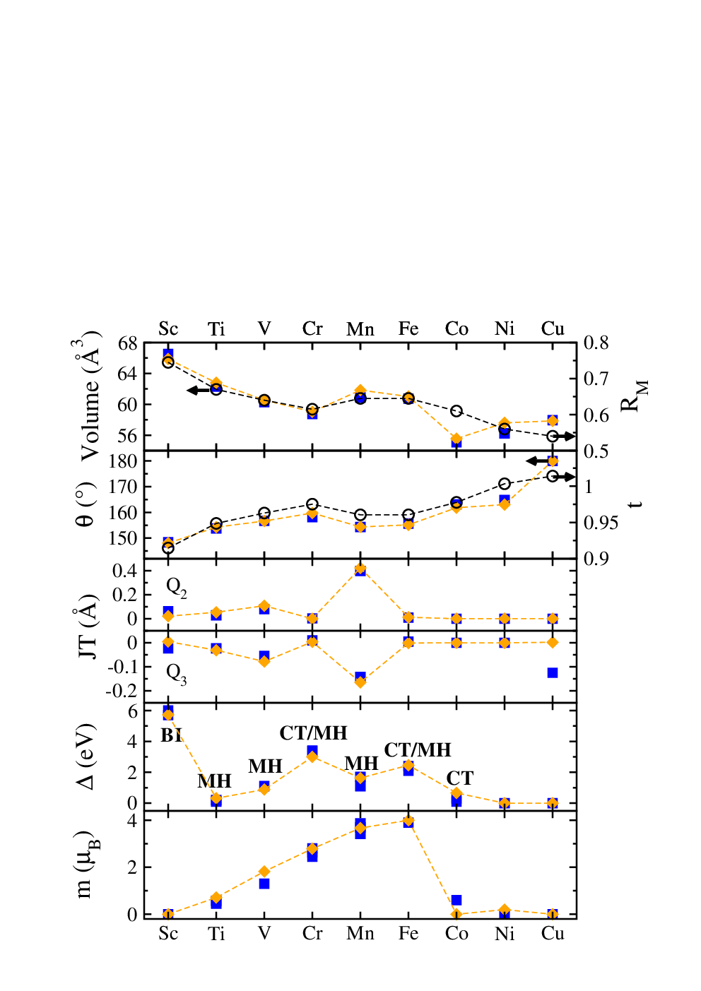
The variation of the band gaps with the species shown in Fig. 25 is rather complex and in line with the earlier observation of Arima[7, 203]: we observe a general tendency of the MH gap to increase as the TM atomic number increases, whereas the CT gaps follow an opposite behavior. As expected, there is an apparent correlation between the trend of the band gaps and the optimum fraction of exact exchange displayed in Fig. 23, especially . In LDA+U language this behavior is interpreted as a correlation between the strength of the effective Coulomb interaction U and the band gap (this become particularly evident by comparing the curve in Fig.25 with Fig. 2 in Ref. 55 showing the changes of the effective U with respect to ).

In Fig. 26 we collect the bandstructures of LaO3 obtained using the optimum values showing the variation of the electronic dispersion across the whole series. Starting from the band insulator LaScO3 the addition of one electron creates an highly localized state right below in LaTiO3. The gradual filling of this manifold leads to a continuous increase of the band width from (LaTiO3) to (LaCrO3), connected with a gradual increase of the crystal field splitting. In LaMnO3 the fully occupied band is pushed down in energy and the valence band maxima is dominated by the half-filled subbands. The orbital gets completely filled in LaFeO3 which is the last member of the series having a predominantly MH gap. The inclusion of one additional electron yields a sudden change of the bandstructure manifested by a high increase of - hybridization and bandwidth around EF. which finally lead to the onset of a metallic state in LaNiO3 and LaCuO3.
Three members of the LaO3 family (LaTiO3, LaVO3, and LaMnO3) are known to display orbital-ordering (OO) associated with the partially filled and orbitals located on top of the valence band (these states are demarcated by thick lines in Fig. 26). A visual representation of the OO states derived from the ’optimum’ HSE wavefunctions is shown in Fig.27 in terms of charge density isosurfaces of the highest occupied states. In the following we describe briefly the most important characteristics of the observed OO states.
(i) In LaTiO3, where the OO originates from the single electron, the lobes have a quasi cigar-like shape with asymmetric contributions along the two main directions, indicating an almost identical occupation of the three , , and shells. Co-planar lobes are arranged in a chessboard-like way with a sign alternation along z, in good agreement with previously reported theoretical[170, 112, 204] and experimental works [148, 205]. There is a clear connection between this chessboard-like Ti ordering and the JT structural instability, which is manifested by the tendency of the occupied state to lie along the longer Ti-O bond. This also explains why the chessboard-like OO in LaTiO3 is not as much evident as in LaMnO3: in LaTiO3 the difference between the distinct Ti-O bondlengths Ti-Os Ti-Om Ti-Ol, quantified by the JT parameters Q2 and Q3, is about one order of magnitude smaller than in LaMnO3 (see Table 3 and Table 6).
(ii) The V3+ ions in LaVO3 can accommodate two electrons in the three possible orbital states , , and . The spins are arranged according to the C-type ordering, whereas the OO state is found to be G-type, in accordance with the Goodenough-Kanamori rules[206] and in agreement with x-ray diffraction[207] and previous GGA[60] and HF[104] calculations. The distribution of the orbitals in the G-type OO state follows the cooperative JT-induced V-O bond-alternation in the xy plane and along the z axis, i.e. the charge density in one specific V site is rotated by 90∘ with respect to that in the 6 neighboring V sites (four in-plane and two in the adjacent vertical planes). As already observed for LaTiO3, the orbitals are preferentially occupied along the long-bond direction.
(iii) The C-type OO in LaMnO3, originating from the singly occupied state of the Mn+3 3 electrons in the high-spin configuration has been extensively studied both experimentally[208, 209, 183], and theoretically[179, 180]. We have also recently addressed this issue throughout a maximally localized Wannier functions representation of the states[41]. This C-type OO state can be written in the form with the sign of alternating along and and repeating along , as correctly represented by our HSE charge density plots.
For comparison we show in Fig. 28 the similar charge density isosurfaces calculated for LaCrO3 and LaFeO3, in which the half-filling of the and orbitals inhibit any orbital flexibility. As expected there is no sign of orbital ordering.
We conclude this section with a comparison of the calculated density of valence and conduction states with available x-ray photoemission and x-ray adsorption spectra. This is summarized in Fig. 29. The overall picture is satisfactory in terms of bandwidth, intensity and peaks position, though some sizable deviations are visible for LaCrO3, LaFeO3 and for the metallic compounds LaCuO3 and LaNiO3. These differences between theory and experiment should be attributable to the approximations included in the adopted computational scheme, as mentioned in the previous section.


V SUMMARY AND CONCLUSIONS
In summary, we have studied the ground state properties of the perovskite series LaO3 by means of screened hybrid DFT following the HSE formulation, based on the inclusion of a fraction of exact HF exchange in the short range Coulomb kernel of the underlying semilocal PBE exchange-correlation functional. In particular, we have investigated the role of the HSE mixing parameter on the (i) structural parameters (Volume, JT/GFO distortions, lattice parameters and unit cell symmetry) (ii) electronic character (band gap, DOS, and bandstructure), and (iii) spin orderings and magnetic moment, as a function of the gradual filling of the manifold from LaScO3 () to LaCuO3 (: ).
On the basis of a computational fitting of the most relevant experimentally available data we have derived a set of mixing factors which leads to an accurate qualitative and quantitative description of the physical behavior of all members of the representative LaO3 family. It is found that, apart from LaScO3, the ’optimum’ values of () are significantly smaller than the routinely used standard choice =0.25, especially for the end members ( LaScO3: =0.25; LaTiO3 & LaVO3: =0.10-0.15; LaCrO3, LaMnO3, and LaFeO3: =0.15; LaCoO3: =0.05; LaNiO3 & LaCuO3: =0.0, i.e. for these two cases PBE is better than HSE ). This can be understood by correlating the changes of from Sc to Cu with the corresponding values of the inverse dielectric constant , and by considering that a certain degree of screening is already included by construction in the HSE functional throughout the screening length , at variance with the unscreened parent hybrid functional PBE0 (for which ). This suggests that the ’optimum’ value of in HSE should be smaller than the corresponding PBE0 one: in our specific case it is proposed that the difference between and should about 0.05-0.07, but a more detailed analysis on the influence of is required to achieve more accurate and comprehensive conclusions.

An alternative way to obtain a set of optimum is the fitting of the bandgap only, by applying the practical recipe represented by Eq. 8. However, though this procedure has the clear advantage of reducing considerably the computational cost, it can lead to an erroneous description of other properties (for example the best-bandgap in LaTiO3 stabilizes the wrong spin ordering) and can only be applied under the assumption that the wavefunction does not change with .
For what concerns the description of the modulation of the electronic and magnetic properties across the LaO3 series, we found that for all insulating compounds (=Sc to Co) HSE is capable to capture the localization of the / orbitals and to provide a consistent and quantitatively satisfactory description of all considered quantities, thereby improving the deficient DFT based predictions.
For the structural properties, on the other hand, PBE performs rather well, delivering optimized geometry within 1%. The only exception are the JT parameters in LaMnO3, which PBE finds 60% smaller than experiment. HSE cures this limitation, reproducing quite well the critical JT and GFO structural instabilities, and, in general, its application improves even further the overall agreement with experiment as compared to PBE.
The complex nature of the PM correlated metals LaNiO3 and LaCuO3, end members of the LaO3 series, is only marginally accounted for by PBE and rather poorly treated at HSE level. This is mostly due to underlying dynamical correlation effects which cannot be easily treated at DFT/HF level. For these compounds, PBE might be considered to be a good starting point for more elaborated many-body approaches.
VI ACKNOWLEDGMENTS
This research was sponsored by the FP7 European Community grant ATHENA. All calculations have been performed on the Vienna Scientific Cluster (VSC).
References
- [1] N. F. Mott Metal-Insulator Transitions (Taylor & Francis, London, 1990).
- [2] M. Imada, A. Fujimori, and Y. Tokura, Rev. Mod. Phys. 70, 1039 (1998).
- [3] J. G. Bednorz and K. A. Müller, Z. Phys. B 64, 189 (1986).
- [4] R. von Helmolt, J. Wecker, B. Holzapfel, L. Schultz, and K. Samwer, Phys. Rev. Lett. 71, 2331 (1993).
- [5] M. B. Salamon and M. Jaime, Rev. Mod. Phys. 73, 583 (2001).
- [6] K. F. Wang, J. M. Liu, and Z. F. Ren, Adv. Phys. 58, 321 (2009).
- [7] T. Arima, Y. Tokura, and J. B. Torrance, Phys. Rev. B 48, 17006 (1993).
- [8] H. Tanaka and M. Misono, Curr. Opin. Solid State Matter. Sci. 5, 381 (2001).
- [9] J. Suntivich, H. A. Gasteiger, N. Yabuuchi, H. Nakanishi, J. B. Goodenough, and Y. Shao-Horn, Nature Chem. 3, 546 (2011).
- [10] P. Zubko, S. Gariglio, M. Gabay, P. Ghosez, and J.-M. Triscone, Annu. Rev. Condens. Matter Phys. 2, 141 (2011).
- [11] A. P. Ramirez, J. Phys. Condens. Matter 9, 8171 (1997).
- [12] J. M. D. Coey, M. Viret, and S. von Molnár, Adv. Phys. 48, 167 (1999).
- [13] I. Loa, P. Adler, A. Grzechnik, K. Syassen, U. Schwarz, M. Hanfland, G. Kh. Rozenberg, P. Gorodetsky, and M. P. Pasternak, Phys. Rev. Lett. 87, 125501 (2001).
- [14] J.-S. Zhou, J. A. Alonso, A. Muoz, M. T. Fernández-Díaz, and J. B. Goodenough, Phys. Rev. Lett. 106, 057201 (2011).
- [15] A. Asamitsu, Y. Moritomo, Y. Tomioka, T. Arima, and Y. Tokura Nature 373, 407 (1995).
- [16] C.M. Varma, Phys. Rev. B 54, 7328 (1996).
- [17] R. Ramesh and D.G. Sclom, MRS Bulletin 33, 1006 (2008).
- [18] J. Chakhalian, A. J. Millis, and J. Rondinelli, Nature Mat. 11, 92 (2012).
- [19] A. Kudo and Y. Miseki, Chem. Soc. Rev. 38, 253 (2009).
- [20] S. B. Adler, Chem. Rev. 104, 4791 (2004).
- [21] P. W. Anderson, Phys. Rev. 124, 41 (1961).
- [22] O. Gunnarsson and K. Schönhammer, Phys. Rev. Lett. 50, 604 (1983).
- [23] W. Kohn, Rev. Mod. Phys. 71, 1253 (1999).
- [24] W. Kohn and L. J. Sham, Phys. Rev. 140, A1133 (1965).
- [25] W. Metzner and D. Vollhardt, Phys. Rev. Lett. 62, 324 (1989).
- [26] A. Georges, G. Kotliar, W. Krauth and M. J. Rozenberg, Rev. Mod. Phys. 68, 13 (1996).
- [27] G. Kotliar, S. Y. Savrasov, K. Haule, V. S. Oudovenko, O. Parcollet, C. A. Marianetti, Rev. Mod. Phys. 78, 865 (2006).
- [28] I. V. Solovyev, J. Phys.: Condens. Matter 20, 293201 (2008).
- [29] M. Imada and T. Miyake, J. Phys. Soc. Jpn. 79, 112001 (2010).
- [30] P. W. Anderson, Phys. Rev. 115, 2 (1959).
- [31] J. Hubbard, Proc. R. Soc. London, Ser. A 276, 238. (1963); J. Hubbard, ibid. 277, 237 (1964); J. Hubbard, ibid. 281, 401 (1964).
- [32] J. Kanamori, Prog. Theor. Phys. 30, 275 (1963).
- [33] C. J. Calzado, J. Cabrero, J.P. Malrieu, R. Caballol, J. Chem. Phys. 106, 2728 (2002); ibid. 106, 3985 (2002)
- [34] I. D. Prodan, Gustavo E. Scuseria, and Richard L. Martin, Phys. Rev. B 76 033101 (2007).
- [35] I.D.R. Moreira, C.J. Calzado, J.P. Malrieu, F. Illas New J. of Phys. 9 369 (2007).
- [36] V. Bayer, C. Franchini, and R. Podloucky Phys. Rev. B 75 , 035404 (2007)
- [37] G. Fischer, M. Däne, A. Ernst, P. Bruno, M. Lüeders, Z. Szotek, W. Temmerman, and W. Hergert, Phys. Rev. B 80, 014408 (2009).
- [38] C. Boilleau, N. Suaud, R. Bastardis, N. Guihéry and J.-P. Malrieu Theor. Chem. Acc. 126, 231 (2010).
- [39] R. Kováčik and C. Ederer, Phys. Rev. B 81, 245108 (2010).
- [40] R. Kováčik and C. Ederer, Phys. Rev. B 84, 075118 (2011).
- [41] C. Franchini, R. Kováčik, M. Marsman, S. Sathyanarayana Murthy, J. He, C. Ederer, G. Kresse, J. Phys.: Condens. Matter 24, 235602 (2012).
- [42] J. P. Perdew, A. Ruzsinszky, J. Tao, V. N. Staroverov, G. E. Scuseria, and G. I. Csonka, J. Chem. Phys. 123, 062201 (2005).
- [43] R. G. Parr and W. Yang 1989 Density-Functional Theory of Atoms and Molecules (Oxford: Clarendon) (1999).
- [44] V. I. Anisimov, J. Zaanen, and O. K. Andersen, Phys. Rev. B 44, 943 (1991).
- [45] J. P. Perdew and A. Zunger, Phys. Rev. B 23, 5048 (1981).
- [46] A. Svane and O. Gunnarsson, Phys. Rev. Lett. 65, 1148 (1990).
- [47] Z. Szotek, W.M. Temmerman, and H. Winter, Physica B: Cond. Mat. 172, 19 (1991).
- [48] A. Filippetti and N. A. Spaldin, Phys. Rev. B 67, 125109 (2003).
- [49] A. D. Becke, J. Chem. Phys. 98 1372 (1993).
- [50] L. Hedin, Phys. Rev. 139, A796 (1965).
- [51] C. J. Cramer and D. G. Truhlar, Phys. Chem. Chem. Phys. 11 10757 (2009)
- [52] J. Heyd, G.E. Scuseria, and M. Ernzerhof, J. Chem. Phys. 118 8207 (2003); J. Chem. Phys. 124 219906 (2006).
- [53] M. T. Czyżyk and G. A. Sawatzky, Phys. Rev. B 49, 14211 (1994).
- [54] D. D. Sarma, N. Shanthi, S. R. Barman, N. Hamada, H. Sawada, and K. Terakura, Phys. Rev. Lett. 75, 1126 (1995).
- [55] I. Solovyev, N. Hamada, and K. Terakura, Phys. Rev. B 53, 7158 (1996).
- [56] I. Solovyev, N. Hamada, and K. Terakura, Phys. Rev. Lett. 76, 4825 (1996).
- [57] T. Mizokawa and A. Fujimori, Phys. Rev. B 54, 5368 (1996).
- [58] M. A. Korotin, S. Yu. Ezhov, I. V. Solovyev, V. I. Anisimov, D. I. Khomskii, and G. A. Sawatzky, Phys. Rev. B 54, 5309 (1996).
- [59] Z. Yang, Z. Huang, L. Ye, and X. Xie, Phys. Rev. B 60, 15674 (1999).
- [60] H. Sawada, N. Hamada, K. Terakura, and T. Asada, Phys. Rev. B 53, 12742 (1996).
- [61] H. Sawada, Y, Morikawa, K. Terakura, and N. Hamada, Phys. Rev. B 56, 12154 (1997).
- [62] N. Hamada, H. Sawada, I. Solovyev, K. Terakura, Physica B 237, 11 (1997).
- [63] P. Ravindran, A. Kjekshus, H. Fjellvȧg, A. Delin, and O. Eriksson, Phys. Rev. B 65, 064445 (2002).
- [64] D. Muñoz, N. M. Harrison, and F. Illas, Phys. Rev. B 69, 085115 (2004).
- [65] P. Ravindran, R. Vidya, H. Fjellvåg, and A. Kjekshus, J. Cryst. Growth 268, 554 (2004).
- [66] Z. Fang and N. Nagaosa, Phys. Rev. Lett. 93, 176404 (2004).
- [67] R. A. Evarestov, E. A. Kotomin, Yu, A. Mastrikov, D. Gryaznov, E. Heifets, and J. Maier, Phys. Rev. B 72, 214411 (2005).
- [68] M. Sahnoun, C. Daul, O. Haas, and A. Wokaun, J. Phys.: Condens. Matter 17, 7995 (2005).
- [69] S. Okatov, A. Poteryaev, and A. Lichtenstein, Europhys. Lett. 70, 499 (2005).
- [70] G. Trimarchi and N. Binggeli, Phys. Rev. B 71, 035101 (2005).
- [71] E. A. Kotomin, R. A. Evarestov, Yu. A. Mastrikova and J. Maier, Phys. Chem. Chem. Phys. 7, 2346 (2005).
- [72] I. V. Solovyev, Phys. Rev. B 74, 054412 (2006).
- [73] K. Knížek, Z. jiraḱ, J. Hejtmánek, and P. Novák, J. Phys.: Condens. Matter 18, 3285 (2006).
- [74] H. S. Ahn, D. D. Cuong, J. Lee, S. W. Han, J. Korean Phys. Soc. 49, 1536 (2006).
- [75] K. P. Ong, P. Blaha, and P. Wu, Phys. Rev. B 77, 073102 (2008).
- [76] Y. Nohara, A. Yamasaki, S. Kobayashi, and T. Fujiwara, Phys. Rev. B 74, 064417 (2006).
- [77] H. Hsu, K. Umemoto, M. Cococcioni, and R. Wentzcovitch, Phys. Rev. B 79, 125124 (2009).
- [78] Y. Nohara, S. Yamamoto, and T. Fujiwara, Phys. Rev. B 79, 195110 (2009).
- [79] J. W. Zwanziger, Phys. Rev. B 79, 033112 (2009).
- [80] K. Kníz̀ek, Z. Jirák, J. Hejtmánek, P. Novák, and W. Ku, Phys. Rev. B. 79, 014430 (2009).
- [81] H. Hsu, P. Blaha, R. M. Wentzcovitch, and C. Leighton, Phys. Rev. B. 82, 100406(R) (2010).
- [82] D. Gryaznov, R. A. Evarestov, and J. Maier, Phys. Rev. B 82, 224301 (2010).
- [83] T. Hashimoto, S. Ishibashi, and K. Terakura, Phys. Rev. B 82, 045124 (2010).
- [84] A. Laref, and S. J. Lou, J. Phys. Soc. Jpn. 79, 064702 (2010).
- [85] C. Ederer, T. Harris, R. Kováčik, Phys. Rev. B 83, 054110 (2011).
- [86] G. Guo, I. Grinberg, A. M. Rappe, and J. M. Rondinelli, Phys. Rev. B 84, 144101 (2011).
- [87] E. A. Ahmad, L. Liborio, D. Kramer, G. Mallia, A. R. Kucernak, and N. M. Harrison, Phys. Rev. B 84, 085137 (2011).
- [88] J. Hong, A. Stroppa, J. Íñiguez, S. Picozzi, and D. Vanderbilt, Phys. Rev. B 85, 054417 (2012).
- [89] J. He, M. Chen, X.-Q. Chen, C. Franchini, Phys. Rev. B 85, 195135 (2012).
- [90] K. Momma and F. Izumi, J. Appl. Crystallogr. 41, 653 (2008).
- [91] W. Y. Hu, M. C. Qian, Q. Q. Zhang, H. Q. Lin, and H. K. Wong, Phys. Rev. B 61, 1223 (2000).
- [92] E. R. Ylvisaker, W. E. Pickett, and K. Koepernik, Phys. Rev. B 79, 035103 (2009).
- [93] J. P. Perdew, K. Burke and M. Ernzerhof, Phys. Rev. Lett. 77, 3865 (1996).
- [94] Y. S. Su, T. A. Kaplan, S. D. Mahanti, and J. F. Harrison, Phys. Rev. B 61, 1324 (2000).
- [95] M. Mochizuki and M. Imada, New J. Phys. 6, 154 (2004).
- [96] E. Pavarini, A. Yamasaki, J. Nuss, and O. K. Andersen, New J. Phys. 7, 188 (2005).
- [97] X.-F. Hao, A. Stroppa, A. Filippetti, S. Picozzi, C. Franchini, Phys. Rev. B 86, 014116 (2012).
- [98] P. Rivero, I. de P. R. Moreira, G. E. Scuseria, and F. Illas, Phys. Rev. B 79, 245129 (2009).
- [99] P. Rivero, I. de P.R. Moreira, and F. Illas Phys. Rev. B 81, 205123 (2010).
- [100] O. Gunnarsson, O. K. Andersen, O. Jepsen, J. Zaanen, Phys. Rev. B 39, 1708 (1989).
- [101] V. I. Anisimov and O. Gunnarsson, Phys. Rev. B 43, 7570 (1991).
- [102] F. Aryasetiawan, M. Imada, A. Georges, G. Kotliar, S. Biermann, A.I Lichtenstein, Phys. Rev. B 70, 195104 (2004).
- [103] M. Cococcioni and S. de Gironcoli, Phys. Rev. B 71, 035105 (2005).
- [104] I. V. Solovyev, Phys. Rev. B 73, 155117 (2006).
- [105] K. Karlsson, F. Aryasetiawan, and O. Jepsen, Phys. Rev. B 81, 245113 (2010).
- [106] M. A. L. Marques, J. Vidal, M. J. T. Oliveira, L. Reining, and S. Botti, Phys. Rev. B 83, 035119 (2011).
- [107] J. Paier, R. Hirschl, M. Marsman, and G. Kresse, J. Chem. Phys. 122, 234102 (2005).
- [108] T. Archer, D. Chaitanya, S. Sanvito, J. He, C. Franchini, A. Fllippetti, P. Delugas, D. Puggioni, V. Fiorentini, R. Tiwari, and P. Majumdar, Phys. Rev. B 84, 115114 (2011).
- [109] F. Iori, M. Gatti, and A. Rubio, Phys. Rev. B 85, 115129 (2012).
- [110] J. P. Perdew, M. Ernzerhof, and K. Burke, J. Chem. Phys. 105, 9982 (1996).
- [111] J. Paier, M. Marsman, K. Hummer, G. Kresse, I. C. Gerber, and J. G. Ańgyań, J. Chem. Phys. 124, 154709 (2006).
- [112] A. Filippetti, C. D. Pemmaraju, S. Sanvito, P. Delugas, D. Puggioni, and V. Fiorentini, Phys. Rev. B 84, 195127 (2011).
- [113] H. Zenia, G. A. Gehring, and W. M. Temmerman, New J. Phys. 7, 257 (2005).
- [114] A. Filippetti and V. Fiorentini, Eur. Phys. J. B 71, 139 (2009).
- [115] M. Shishkin, M. Marsman, and G. Kresse, Phys. Rev. Lett. 99, 246403 (2007).
- [116] C. Franchini, A. Sanna, M. Marsman, and G. Kresse, Phys. Rev. B 81, 085213 (2010).
- [117] G. Kresse and J. Hafner, Phys. Rev. B 48, 13115 (1993).
- [118] G. Kresse and J. Furthmüller, Comput. Mater Sci. 6, 15 (1996).
- [119] P. E. Blöchl, Phys. Rev. B 50, 17953 (1994).
- [120] G. Kresse and D. Joubert, Phys. Rev. B 59, 1758 (1999).
- [121] J. Heyd, J. E. Peralta, G. E. Scuseria, and R. L. Martin, J. Chem. Phys. 123, 174101 (2005).
- [122] I. C. Gerber, J. G. Ángyán, M. Marsman, G. Kresse J. Chem. Phys. 127, 054101 (2007).
- [123] M. Marsman, J. Paier, A. Stroppa, and G. Kresse, J. Phys.: Condens. Matter 20, 064201 (2008).
- [124] C. Franchini, R. Podloucky, J. Paier, M. Marsman, G. Kresse, Phys. Rev. B 75, 195128 (2007).
- [125] C. Franchini, T. Archer, J. He, X Chen, A. Filippetti, S. Sanvito, Phys. Rev. B 83, 220402 (2011).
- [126] A. Stroppa, S. Picozzi, Phys. Chem. Chem. Phys. 12, 5405 (2010).
- [127] A. Stroppa and G. Kresse New J. Phys. 10 063020 (2004).
- [128] C. Franchini, J. Zabloudil, R. Podloucky, F. Allegretti, F. Li, S. Surnev, F.P. Netzer, J. of Chem. Phys. 130, 124707 (2009).
- [129] J. B. Varley, A. Janotti, C. Franchini, and C. G. Van de Walle, Phys. Rev. B 85, 081109(R) (2012).
- [130] I. de P. R. Moreira, F. Illas, and R. L. Martin, Phys. Rev. B 65, 155102 (2002), and references therein.
- [131] X. Feng, and N. M Harrison, Phys. Rev. B 70, 092402 (2004).
- [132] A. V. Krukau, O. A. Vydrov, A. F. Izmaylov, and G. Scuseria, J. Chem. Phys. 125, 224106 (2006).
- [133] F. Gygi and A. Baldereschi, Phys. Rev. Lett. 62, 2160 (1989).
- [134] S. J. Clark and J. Robertson, Phys. Rev. B 82, 085208 (2010).
- [135] A. Alkauskas, P. Broqvist, A. Pasquarello, Phys. Status solidi (b) 248, 775 (2010).
- [136] C. Gutle, A. Savin, J. B. Krieger, and J. Chen, Int. J. Quantum Chem. 75, 885 (1999).
- [137] F. Tran and P. Blaha, Phys. Rev. Lett. 102, 226401 (2009).
- [138] R. W. Nunes and X. Gonze, Phys. Rev. B 63, 155107 (2001).
- [139] M. J. Han, T. Ozaki, and J. Yu, Phys. Rev. B 73, 045110 (2006).
- [140] I. V. Solovyev and P. H. Dederichs Phys. Rev. B 49, 6736 (1994).
- [141] A. Chainani, M. Mathew, and D. D. Sarma, Phys. Rev. B 46, 9976 (1992).
- [142] T. Mizokawa and A. Fujimori, Phys. Rev. 51, 12880 (1995).
- [143] D. D. Sarma and A. Chainani, J. Solid State Chem. 111, 208 (1994).
- [144] T. Saitoh, A. E. Bocquet, T. Mizokawa, H. Namatame, A. Fujimori, M. Abbate, Y. Takeda, M. Takano, Phys. Rev. B 51, 13942 (1995).
- [145] M. Abbate, J. C. Fuggle, A. Fujimori, L. H. Tjeng, C. T. Chen, R. Potze, G. A. Sawatzky, H. Eisaki and S. Uchida, Phys. Rev. B 47, 16124 (1993).
- [146] C. Franchini, V. Bayer, R. Podloucky, J. Paier, and G. Kresse, Phys. Rev. B 72, 045132 (2005).
- [147] S. Geller, Acta Cryst. 10, 243 (1957).
- [148] M. Cwik, T. Lorenz, J. Baier, R. Müller, G. André, F. Bourée, F. Lichtenberg, A. Freimuth, R. Schmitz, E. Müller-Hartmann, and M. Braden, Phys. Rev. B 68, 060401 (2003).
- [149] D. A. Maclean, H. N. Ng, and J. E. Greedan, J. Solid State Chem. 30, 35 (1979).
- [150] P. Bordet, C. Chaillout, M. Marezio, Q. Huang, A. Santoro, S-W. Cheong, H. Takagi, C. S. Oglesby, B. Batlogg, J. Solid State Chem. 106, 253 (1993).
- [151] C. P. Khattak and D. E. Cox, Mater. Res. Bull. 12, 463 (1977).
- [152] K. Tezuka, Y. Hinatsu, A. Nakamura, T. Inami, Y. Shimojo, and Y. Morii, J. Solid State Chem. 141, 404 (1998).
- [153] G. Li, X. Kuang, S. Tian, F. Liao, X. Jing, Y. Uesu, and K. Kohn, J. Solid State Chem. 165, 381 (2002).
- [154] J. B. A. A. Elemans, B. van Laar, K. R. van der Veen, and B. O. Loopstra, J. Solid State Chem. 3, 238 (1971).
- [155] S. E. Dann, D. B. Currie, and M. T. Weller, M. F. Thomas, and A. D. Al-Rawwas, J. Solid State Chem. 109, 134 (1994).
- [156] P. G. Radaelli and S. W. Cheong, Phys. Rev. B 66, 094408 (2002).
- [157] G. Thornton, B. C. Tofield, and A. W. Hewat, J. Solid State Chem. 61, 301 (1986).
- [158] O. Haas, R. P. W. J. Struis, and J. M. McBreen, J. Solid State Chem. 177, 1000 (2004).
- [159] J. L. García-Muñoz, J. Rodrǵuez-Carvajal, P. Lacorre, J. B. Torrance, Phys. Rev. B 46, 4414 (1992).
- [160] S. Darracq, S. Matar, and G. Demzeau, Solid State Comm. 85, 961 (1993).
- [161] J. F. Bringley, B. A. Scott, S. J. La Placa, T. R. McGuire, and F. Mehran, M. W. McElfresh, D. E. Cox, Phys. Rev. B 47, 15269 (1993).
- [162] I. de P. R. Moreira and F. Illas, Phys. Chem. Chem. Phys. 8, 1645 (2006).
- [163] V. V. Afans’ev, A. Stesmans, C. Zhao, M. Caymax, T. Heeg, J. Schubert, Y. Jia, D. G. Schlom, and G. Lucovsky, Appl. Phys. Lett. 85, 5917 (2004).
- [164] J. Hemberger, H. -A. Krug von Nidda, V. Fritsch, J. Deisenhofer, S. Lobina, T. Rudolf, P. Lunkenheimer, F. Lichtenberg, A. Loidl, D. Druns, and B. Büchner, Phys. Rev. Lett. 91, 066403 (2003).
- [165] B. Keimer, D. Casa, A. Ivanov, J. W. Lynn, M. v. Zimmermann, J. P. Hill, D. Gibbs, Y. Taguchi, and Y. Tokura, Phys. Rev. Lett. 85, 3946 (2000).
- [166] Y. Okimoto, T. Katsufuji, Y. Okada, T. Arima, and Y. Tokura, Phys. Rev. B 51, 9581 (1995).
- [167] S. V. Streltsov, A. S. Mylnikova, A. O. Shorikov, Z. V. Pchelkina, D. I. Khomskii, and V. I. Anisimov, Phys. Rev. B 71, 245114 (2005).
- [168] H. Fujitani and S. Asano, Phys. Rev. B 51, 2098 (1995).
- [169] H. Sawada and K. Terakura, Phys. Rev. B 58, 6831 (1998).
- [170] E. Pavarini, S. Biermann, A. Poteryaev, A. I. Lichtenstein, A. Georges, and O. K. Andersen, Phys. Rev. Lett. 92, 176403 (2004).
- [171] I. Solovyev, Phys. Rev. B 69, 134403 (2004).
- [172] J. P. Goral and J. E. Greedan, J. Magn. Magn. Mater. 37, 315 (1983).
- [173] D. Gryaznov, E. Heifetsa and E. Kotomin, Phys. Chem. Chem. Phys. 14, 4482 (2012)
- [174] H. Roth, Ph. D. thesis, Universität zu Köln (Germany), 2008, http://kups.ub.uni-koeln.de/2335/.
- [175] V. G. Zubkov, G. V. Bazuev, V. A. Parelyaev, and G. P. Shveikin, Sov. Phys. Solid State 15, 1078 (1973).
- [176] W. K. Koehler and E. O. Wollan, J. Phys. Chem. Solids 2, 100 (1957).
- [177] E. F. Bertaut, J. Mareschal, G. De Vries, R. Aleonard, R. Pauthenet, J. P. Rebouillat, and V. Zarubicka, IEEE Trans. Magn. 2, 453 (1966).
- [178] N. Sakai, H. Fjellvaĝ, and B. C. Hauback, J. Solid State Chem. 121, 202 (1996).
- [179] W-G. Yin, D. Volja and W. Ku, Phys. Rev. Lett. 96, 116405 (2006).
- [180] E. Pavarini and E. Koch , Phys. Rev. Lett. 104, 086402 (2010).
- [181] J. H. Jung, K. H. Kim, D. J. Eom, T. W. Noh, E. J. Choi, J. Yu, Y. S. Kwon, Y. Chung, Phys. Rev. B 55, 15489 (1997).
- [182] J. H. Jung, K. H. Kim, T. W. Noh, E. J. Choi, J. Yu, Phys. Rev. B 57, R11043 (1998).
- [183] R. Krüger, B. Schulz, S. Naler, R. Rauer, D. Budelmann, J. Bäckström, K.H. Kim, S-W. Cheong, V. Perebeinos, and M. Ru bhausen, Phys. Rev. Lett. 92, 097203 (2004).
- [184] F. Moussa, M. Hennion, J. Rodríguez-Carvajal, H. Moudden, L. Pinsard, and A. Revcolevschi, Phys. Rev. B 54, 15149 (1996).
- [185] B. C. Hauback, H. Fjellvåg, and N. Sakai, J. Solid State Chem. 124, 43 (1996).
- [186] J. Rodríguez-Carvajal, M. Hennion, F. Moussa, A. H. Moudden, L. Pinsard, and A. Revcolevschi, Phys. Rev. B 57, R3189 (1998).
- [187] R. L. White, J. Appl. Phys. 40, 1061 (1969).
- [188] M. B. Bellakki, B. J. Kelly, V. Manivannan, J. Alloys Compd. 489, 64 (2010).
- [189] X. D. Zhou, L. R. Pederson, Q. Cai, J. Yang, B. J. Scarfino, M. Kim, W. B. Yelon, W. J. James, H. U. Anderson, and C. Wang, J. Appl. Phys. 99, 08M918 (2006).
- [190] H. Wadati, D. Kobayashi, H. Kumigashira, K. Okazaki, T. Mizokawa, A. Fujimori, K. Horiba, M. Oshima, N. Hamada, M. Lippmaa, M. Kawasaki, and H. Koinuma, Phys. Rev. B 71, 035108 (2005).
- [191] J. B. Goodenough, Localized to Itinerant Electronic Transition in Perovskite Oxides (Springer, New York, 2001) (and references therein).
- [192] C. N. R. Rao, Md. Motin Seikh, and C. Narayana, Top. Curr. Chem. 234, 1 (2004) and references therein.
- [193] S. Yamaguchi, Y. Okimoto, H. Taniguchi, and Y. Tokura, Phys. Rev. B 53, R2926 (1996).
- [194] K. Sreedhar, J. M. Honig, M. Darwin, M. McElfresh, P. M. Shand, J. Xu, B. C. Crooker, and J. Spalek, Phys. Rev. B 46, 6382 (1992).
- [195] D. D. Sarma, N. Shanthi, and P. Mahadevan, J. Phys. Condens.: Matter 6, 10467 (1994).
- [196] V. I. Anisimov, D. Bukhvalov, and T.M. Rice, Phys. Rev. B 59, 7901 (1999).
- [197] M. K. Stewart, C.-H. Yee, Jian Liu, M. Kareev, R. K. Smith, B. C. Chapler, M. Varela, P. J. Ryan, K. Haule, J. Chakhalian, and D. N. Basov, Phys. Rev. B 83, 075125 (2011).
- [198] P. Hansmann, A. Toschi, X. Yang, O. K. Andersen, and K. Held, Phys. Rev. B 82, 235123 (2010).
- [199] X. Deng, M. Ferrero, J. Mravlje, M. Aichhorn, and A. Georges, Phys. Rev. B 85, 125137 (2012).
- [200] T. Mizokawa and A. Fujimori, H. Namatame, Y. Takeda, M. Takano, Phys. Rev. 57, 9550 (1998).
- [201] K. Okada and A. Kotani, Phys. Status Solidi (b) 68, 666 (1999).
- [202] G. Yalovega and A. V. Soldatov, phys. stat. sol. (b) 218, 455 (2000).
- [203] T. Arima and Y. Tokura, J. Phys. Soc. Jpn. 64, 2488 (1995).
- [204] M. Mochizuki and M. Imada, Phys. Rev. Lett. 91, 167203 (2003).
- [205] T. Kiyama and M. Itoh, Phys. Rev. Lett. 91, 167202 (2003).
- [206] J. B. Goodenough, Prog. Solid State Chem. 5, 145 (1971).
- [207] Y. Ren, A. A. Nugroho, A. A. Menovsky, J. Strempfer, U. Rütt, F. Iga, T. Takabatake, C.W. Kimball, Phys. Rev. B 67, 014107 (2003).
- [208] Y. Murakami, J.P. Hill, D. Gibbs, M. Blume, I. Koyama, M. Tanaka, H. Kawata, T. Arima, Y. Tokura, K. Hirota, and Y. Endoh, Phys. Rev. Lett. 81, 582 (1998).
- [209] N. N. Kovaleva, A. V. Boris, C. Bernhard, A. Kulakov, A. Pimenov, A. M. Balbashov, G. Khaliullin, and B. Keimer, Phys. Rev. Lett. 93, 147204 (2004).
- [210] M. Nakamura, T. Yoshida, K. Mamiya, A. Fujimori, Y. Taguchi, and Y. Tokura, Mater. Sci. Eng., B 68, 123 (1999).
- [211] K. Maiti and D. D. Sarma, Phys. Rev. B 61, 2525 (2000).
- [212] D. D. Sarma, N. Shanthi, and P. Mahadevan, Phys. Rev. B 54, 1622 (1996).
- [213] M. Abbate, G. Zampieri, F. Prado, A. Caneiro, J. M. Gonzalez-Calbet, and M. Vallet-Regi, Phys. Rev. B 65, 155101 (2002).