Quark condensate for various heavy flavors

As it is well known, the so-called chiral SU${}_{L}(N_{\rm f})\times$SU${}_{R}(N_{\rm f})$ symmetry of the classical action of QCD with $N_{\rm f}$ massless quark flavors is spontaneously broken at the quantum level, with the order parameter for this symmetry breaking being the quark condensate $\langle\bar{\psi}\psi\rangle$. Together with confinement, which is characterized by the gluon condensate $\langle(gF_{\mu\nu}^{a})^{2}\rangle$, chiral-symmetry breaking is one of the two most important non-perturbative phenomena in QCD. A natural question can be posed as whether these phenomena are interrelated or not. An affirmative answer to this question would imply proportionality between the quark and the gluon condensates, which was indeed found in Ref. [1]. The corresponding relation reads

where $T_{g}$ is the vacuum correlation length, at which the two-point gauge-invariant correlation function of gluonic field strengths exponentially falls off. Equation (1) stems from the integration in the QCD partition function over soft gluonic fields in the leading, Gaussian, approximation. Within this approximation, the kernel of the four-quark interaction is defined by the two-point field-strength correlation function with the amplitude $\langle(gF_{\mu\nu}^{a})^{2}\rangle$ and the correlation length $T_{g}$.

Alternatively, if one first integrates in the QCD partition function over the quark fields, one arrives at a gauge-invariant effective action, where the gluonic degrees of freedom are represented in the form of Wilson loops and their correlation functions [2]. An advantageous feature of this approach is that, owing to the color-neutrality of Wilson loops, the calculation of the effective action becomes reduced to the calculation of the world-line integrals in an Abelian gauge theory. When the dynamical quarks which are integrated out are sufficiently heavy, namely their current mass $M$ is larger than $1/T_{g}$, the gluonic field inside the quark trajectory can be treated as nearly constant. In this heavy-quark limit, the one-loop effective action yields the following heavy-quark condensate of a given flavor [3]:

This expression coincides with the one known from the SVZ sum rules [4].

With $M$ decreasing downwards $1/T_{g}$, variations of the gauge field inside the quark trajectory produce corrections to Eq. (2). The aim of the present paper is the calculation of such corrections. They will be obtained by using the approach of Ref. [5], which, for the case of a fermion moving in an arbitrary Abelian gauge field, yields a closed formula for the effective action with two field strengths. Furthermore, it is known that, in addition to the confining interactions of stochastic gluonic fields, there also exist non-confining non-perturbative interactions of those fields, albeit of a relatively small strength (cf. Ref. [6]). Below, we study the influence of such interactions on the heavy-quark condensate. For the case of the simplest, purely exponential, two-point correlation function of gluonic field strengths, we find the interesting phenomenon of a complete independence of the heavy-quark condensate from the non-confining non-perturbative interactions.

The paper is organized as follows. In the next Section, we calculate the quark condensate by accounting in the effective action for the confining interactions of stochastic gluonic fields. In Section III, we generalize this result to the case where non-confining non-perturbative interactions of those fields are taken into account. Section IV provides a summary of the results obtained.

Integrating over the quark fields in the QCD partition function, one arrives at the following one-loop effective action [2, 3, 5]:

Here, $P$ and $A$ stand, respectively, for the periodic and the antiperiodic boundary conditions, so that $\int_{P}\equiv\int_{z_{\mu}(s)=z_{\mu}(0)}$, $\int_{A}\equiv\int_{\psi_{\mu}(s)=-\psi_{\mu}(0)}$, and $M$ is the current quark mass. Since the quark condensate is always associated with a given flavor, we set $N_{\rm f}=1$. The corresponding expression for the quark condensate reads

where $V$ is the Euclidean four-volume occupied by the system, and

is the average over gluonic fields. In the heavy-quark limit of $M\gg 1/T_{g}$, the one-loop approximation becomes exact, leading to Eq. (2) [cf. Ref. [3] and the paragraph after Eq. (13) below]. We notice that Eq. (3) uses the fact that the Yang–Mills field-strength tensor $F_{\mu\nu}^{a}=\partial_{\mu}A_{\nu}^{a}-\partial_{\nu}A_{\mu}^{a}-gf^{abc}A_{\mu}^{b}A_{\nu}^{c}$, which enters the quark spin term in the world-line action, can be recovered by means of the area-derivative operator $\frac{\delta}{\delta\sigma_{\mu\nu}}$ acting on the Wilson loop [7]. By virtue of this fact, all the gauge-field dependence of the effective action becomes encoded in the Wilson loop. The latter is defined by the usual formula $\langle W[z_{\mu}]\rangle=\left<{\rm tr}{\,}{\cal P}{\,}\exp\left(ig\int_{0}^{s}d\tau{\,}T^{a}A_{\mu}^{a}\dot{z}_{\mu}\right)\right>$, where $T^{a}$ is a generator of the SU($N_{c}$)-group in the fundamental representation, and ${\cal P}$ denotes the path ordering.

Since $\langle W[z_{\mu}]\rangle$ is completely determined by the geometric characteristics of the contour $C\equiv z_{\mu}(\tau)$, the calculation of the quark condensate becomes an Abelian problem. In this section, we consider the confining part of $\langle W(C)\rangle$, deferring the study of the subleading non-perturbative non-confining part to the next section. Within the stochastic vacuum model [8], the corresponding area-dependent part of the Wilson loop reads

In this formula, $\Sigma$ is the minimal surface bounded by the contour $C$, and $G\equiv\langle(gF_{\mu\nu}^{a})^{2}\rangle$ is the gluon condensate. Furthermore, we choose the surface element $d\sigma_{\mu\nu}$ in the form of an oriented, infinitely thin triangle built up of the position vector $z_{\mu}(\tau)$ and the differential element $dz_{\mu}=\dot{z}_{\mu}d\tau$, namely $d\sigma_{\mu\nu}(z)=\frac{1}{2}(z_{\mu}\dot{z}_{\nu}-z_{\nu}\dot{z}_{\mu})d\tau$. One can then readily check that $\int d\sigma_{\mu\nu}(z)\int d\sigma_{\mu\nu}(z^{\prime})=\left(\int_{0}^{s}d\tau{\,}\dot{z}_{\mu}z_{\nu}\right)^{2}$, as it should be ¹¹ 1 The latter formula can be proved by rewriting the double surface integral as $$\int d\sigma_{\mu\nu}(x)\int d\sigma_{\mu\nu}(x^{\prime})=-\frac{1}{2}\int d\sigma_{\mu\nu}(x)\int d\sigma_{\mu\rho}(x^{\prime}){\,}\partial_{\nu}^{x}\partial_{\rho}^{x^{\prime}}{\,}(x-x^{\prime})^{2},$$ applying the Stokes’ theorem, which leads to $$\int d\sigma_{\mu\nu}(x)\int d\sigma_{\mu\nu}(x^{\prime})=-\frac{1}{2}\oint dz_{\mu}\oint dz_{\mu}^{\prime}(z-z^{\prime})^{2},$$ and noticing that only the $(zz^{\prime})$-term in $(z-z^{\prime})^{2}$ yields a non-vanishing contribution to the last integral, so that $$\int d\sigma_{\mu\nu}(x)\int d\sigma_{\mu\nu}(x^{\prime})=-\frac{1}{2}\oint dz_{\mu}\oint dz_{\mu}^{\prime}(-2zz^{\prime})=\left(\int_{0}^{s}d\tau{\,}\dot{z}_{\mu}z_{\nu}\right)^{2}.$$ . Then, by virtue of an elementary Fourier transform $\int_{x}{\rm e}^{-\mu|x|+ipx}=\frac{12\pi^{2}\mu}{(p^{2}+\mu^{2})^{5/2}}$, one has

where $\Sigma_{\mu\nu}\equiv\Sigma_{\mu\nu}(x;C)=\frac{1}{2}\int_{0}^{s}d\tau{\,}(z_{\mu}\dot{z}_{\nu}-z_{\nu}\dot{z}_{\mu})\delta(x-z(\tau))$ and $\int_{x}\equiv\int d^{4}x$. The exponential of interest thus reads

where the antisymmetry of $B_{\mu\nu}$ has been used at the final step. One recognizes in this formula a Wilson loop corresponding to the Abelian gauge field

The strength tensor of this field is $F_{\mu\nu}=\partial_{\mu}A_{\nu}-\partial_{\nu}A_{\mu}=B_{\mu\nu}+C_{\mu\nu}$, where $C_{\mu\nu}(z)=\frac{1}{2}z_{\lambda}(\partial_{\mu}B_{\lambda\nu}-\partial_{\nu}B_{\lambda\mu})$. In particular, owing to just the Abelian Stokes’ theorem, it is the strength tensor $F_{\mu\nu}$ which automatically appears in the quark spin term of the effective action, being recovered by the operator $\frac{\delta}{\delta\sigma_{\mu\nu}}$ in Eq. (3).

Accordingly, the one-loop effective action (3) takes the form

with the corresponding Abelian covariant derivative $D_{\mu}=\partial_{\mu}-iA_{\mu}$ entering the formfactor ${\sf F}(\xi)$. In the spinor case at issue, this formfactor reads [5] ${\sf F}(\xi)=\frac{f(\xi)-1}{2\xi}-\frac{1}{4}f(\xi)$, where $f(\xi)=\int_{0}^{1}du{\,}{\rm e}^{u(1-u)\xi}$ and $\xi=sD_{\mu}^{2}$. In what follows, we find convenient to identically represent the formfactor ${\sf F}(\xi)$ in the form

Following the method of Ref. [9], each of the two exponentials in the last expression can be represented as

At the final step of the transformation, by performing an elementary $\alpha$-integration, we obtain for the formfactor ${\sf F}(\xi)$ a compact expression

We now insert this expression into Eq. (9). Since the gauge field enters Eq. (10) only via the exponential ${\rm e}^{y_{\mu}D_{\mu}}$, we obtain for the $B$-average in Eq. (9):

To obtain the last equality in Eq. (11) we have used the fact that $C_{\mu\nu}(0)=0$ ²² 2 Rigorously speaking, the correlation functions $\langle B_{\mu\nu}(0)B_{\mu\nu}(y)\rangle_{B}$ and $\langle B_{\mu\nu}(0)C_{\mu\nu}(y)\rangle_{B}$ contain the phase factor $\exp\left[i\int_{0}^{y}du_{\mu}A_{\mu}(u)\right]$. However, the Taylor expansion of such a phase factor would yield correlation functions of more than two $B_{\mu\nu}$’s. On the other hand, the use of the formfactor ${\sf F}$ corresponds to accounting for only two $B_{\mu\nu}$’s. For this reason, we must approximate the said phase factor by unity.. The correlation functions that enter Eq. (11) now read

and

where we have taken into account that an antisymmetric tensor has 12 components.

The large-$M$ limit at issue corresponds to $\xi\ll 1$ and $\mu|y|\ll 1$, so that $f(\xi)\to 1+\frac{\xi}{6}$, ${\sf F}(\xi)\to-\frac{1}{6}$, and only Eq. (12) contributes to Eq. (11), whereas Eq. (13) does not. Recalling finally the definition of the quark condensate, Eq. (4), we recover Eq. (2).

We will now apply the same method of calculation of the effective action to a derivation of the quark condensate for the smaller values of $M$, down to $M=\mu$. Equations (10)-(13) yield

where “1” in the last bracket stems from Eq. (12), while $\left(-\frac{\mu|y|}{4}\right)$ stems from Eq. (13). Accordingly, by using Eq. (4), we can obtain for the quark condensate the following expression:

The $s$-integration in this formula can be performed exactly. Denoting

we arrive at the following intermediate result:

where $K_{\nu}$’s are the Macdonald functions. The $z$-integration here can still be performed analytically, yielding

where $\langle\bar{\psi}\psi\rangle_{\rm SVZ}$ is given by Eq. (2), and $I(\lambda)$ stands for the following integral:

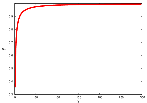
For $\lambda\gg 1$, the leading large-$\lambda$ terms $4+\left(\frac{a}{\lambda}\right)^{2}\cdot\frac{2a^{2}+1}{1-a^{2}}$ yield $I(\lambda)\to 1$. For arbitrary $\lambda$’s, the remaining $u$-integration has been done numerically, with the result plotted in Fig. 1. In particular, we obtain $I(1)\simeq 0.36$, that is, a 64%-decrease in the value of the quark condensate when $M\simeq\mu$. In reality, only the values of $I(\lambda)$ corresponding to $M=M_{c}$, $M_{b}$, and $M_{t}$ are of physical significance. We use the standard quark masses $M_{c}\simeq 1.3{\,}{\rm GeV}$, $M_{b}\simeq 4.2{\,}{\rm GeV}$, and $M_{t}\simeq 173{\,}{\rm GeV}$. The vacuum correlation length in full QCD with light flavors [10], $T_{g}\simeq 0.34{\,}{\rm fm}$, corresponds to $\mu\simeq 580{\,}{\rm MeV}$. This yields

For the alternative case of quenched QCD, that is, SU(3) pure Yang–Mills theory, the vacuum correlation length is [11] $T_{g}\simeq 0.22{\,}{\rm fm}$, which corresponds to $\mu\simeq 897{\,}{\rm MeV}$. For this value of $\mu$, we have

The sets of numbers (17) and (18) illustrate the degree of accuracy of Eq. (2) for various heavy flavors and various values of the vacuum correlation length $T_{g}$. Since the case of heavy quarks considered here constitutes an intermediate case between QCD with light quarks and quenched QCD, the genuine value of $I(M_{f}/\mu)$, for a given heavy flavor $f$, lies somewhere in between the two corresponding values of $I(M_{f}/\mu)$ listed in Eqs. (17) and (18). In any case, we can conclude that Eq. (2) is inapplicable to the $c$-quark, since it can develop up to 53%-corrections [cf. $I(M_{c}/\mu)$ from Eq. (18)]. We notice that a qualitatively similar conclusion has been drawn in Ref. [12], where the leading correction to Eq. (2) has been evaluated through a non-perturbative gluon propagator in the Fock–Schwinger gauge. Finally, setting in Eq. (2) a certain heavy flavor $f$, and denoting $\langle\bar{\psi}\psi\rangle_{{\rm SVZ},f}\equiv-\frac{G}{48\pi^{2}M_{f}}$, we can write, instead of Eq. (16),

For an illustration, we plot in Fig. 2 the ratio (19) for the case of $f=b$ and $T_{g}=0.34{\,}{\rm fm}$, up to $M=M_{b}$. In accordance with the intuitive expectations about the behavior of $\langle\bar{\psi}\psi\rangle$ with $M$, we observe a monotonic decrease of $|\langle\bar{\psi}\psi\rangle|$ with the increase of $M$.

In addition to the confining interactions of stochastic background Yang–Mills fields, which lead to the Wilson loop in the form of Eq. (6), there also exist non-confining non-perturbative interactions of those fields. In this section, we demonstrate the interesting phenomenon of complete independence of the quark condensate from such interactions, provided they exhibit exponential correlations.

To account for the non-confining non-perturbative interactions, one represents the full two-point correlation function of gluonic field strengths in the form [6, 8, 13]

Here, $\kappa\in[0,1]$ is some parameter, which defines the relative strength of the confining and the non-confining non-perturbative interactions. The lattice simulations in the SU(3) Yang–Mills theory yield the value of $\kappa=0.83\pm 0.03$ (cf. Ref. [6]), which means that the relative contribution of the non-confining non-perturbative interactions amounts to only 17%. Expressing the Wilson loop via the correlation function $\left<g^{2}F_{\mu\nu}^{a}(0)F_{\lambda\rho}^{b}(x)\right>$ through the non-Abelian Stokes’ theorem and the cumulant expansion [8], and using the above parametrization of $\left<g^{2}F_{\mu\nu}^{a}(0)F_{\lambda\rho}^{b}(x)\right>$, one obtains the following generalization of Eq. (6):

The non-confining non-perturbative interactions produce in the Wilson loop a term with the double contour integral, which initially has the form (cf. Ref. [13]) $\frac{1-\kappa}{2}\oint_{C}dx_{\mu}\oint_{C}dx_{\mu}^{\prime}\int\limits_{(x-x^{\prime})^{2}}^{\infty}d\tau{\,}{\rm e}^{-\mu\sqrt{\tau}}$. The corresponding expression in Eq. (20) resulted from the $\tau$-integration in this formula.

Much as for the surface-dependent part of the Wilson loop, for the contour-dependent part we can also use some elementary Fourier transform, namely $\int_{x}(1+\mu|x|){\rm e}^{-\mu|x|+ipx}=\frac{60\pi^{2}\mu^{3}}{(p^{2}+\mu^{2})^{7/2}}$, to represent it as

where $j_{\mu}^{x}\equiv j_{\mu}(x;C)=\oint_{C}dx_{\mu}(\tau)\delta(x-x(\tau))$. Further introducing a notation for the mean value $\left<\cdots\right>_{h}=\int{\cal D}h_{\mu}{\,}{\rm e}^{-\frac{2N_{c}}{5\pi^{2}(1-\kappa)\mu G}\int_{x}h_{\mu}(-\partial^{2}+\mu^{2})^{7/2}h_{\mu}}(\cdots)$, we notice that the full Wilson loop (20) can be written as a product of two averages:

This equation generalizes Eq. (7) to the case where the non-confining non-perturbative interactions are also taken into account. Accordingly, the auxiliary Abelian gauge field (8) becomes now $A_{\nu}(z)=\frac{1}{2}z_{\mu}B_{\mu\nu}(z)+h_{\nu}(z)$. Its strength tensor reads $F_{\mu\nu}=B_{\mu\nu}+C_{\mu\nu}+H_{\mu\nu}$, where $H_{\mu\nu}=\partial_{\mu}h_{\nu}-\partial_{\nu}h_{\mu}$. Furthermore, Eq. (11) also gets modified as

where we have denoted $\langle\langle\cdots\rangle_{B}\rangle_{h}$ as just $\langle\cdots\rangle_{B,h}$. The appearing additional correlation function $\langle H_{\mu\nu}(0)H_{\mu\nu}(y)\rangle_{h}$ can be readily calculated by means of the formula

The result reads

Using now Eqs. (12) and (13), with $G$ replaced by $\kappa G$, we observe a remarkable mutual cancellation among all the $\kappa$-dependent contributions. Namely, we obtain

Thus, Eq. (14), with $\langle\cdots\rangle_{B}$ replaced by $\langle\cdots\rangle_{B,h}$, stays unchanged, and so does the resulting quark condensate.

The question whether the obtained cancellation among the $\kappa$-dependent contributions is specific for the above-considered exponential ansatz for the correlation function $\left<g^{2}F_{\mu\nu}^{a}(0)F_{\lambda\rho}^{b}(x)\right>$, or it holds equally well for other ansätze (such as e.g. the Gaussian one), requires a separate study, which lies beyond the scope of the present paper. We only notice that, even in the absence of such a cancellation, the contribution of non-confining non-perturbative interactions is always suppressed, in comparison with the contribution of confining interactions, by a relative factor of $\frac{1-\kappa}{\kappa}\simeq 0.2$.

The aim of the present paper was to find a relation between the quark and the gluon condensates, which would yield, for various heavy flavors, corrections to the known Eq. (2). The corrections thus obtained, given by Eqs. (17) and (18), show that Eq. (2) applies with a good accuracy only to the $t$-quark. Rather, for the $b$-quark, the corrections are $\sim 20\%$, while for the $c$-quark they can be as large as $\sim 50\%$, thereby making Eq. (2) inapplicable to the $c$- and the $s$-quarks. Also, as one can see from Fig. 1, when the continuously varied current quark mass $M$ reaches the value of the inverse vacuum correlation length $\mu$, the absolute value of the quark condensate decreases by 64% compared to the value provided by Eq. (2).

We have used in our calculations the most general ansatz for the Wilson loop, which is provided by the stochastic vacuum model and accounts for the confining and non-perturbative non-confining interactions of the stochastic gluonic fields. The corresponding two-point surface-surface and contour-contour self-interactions of the Wilson loop can be represented as being mediated by an auxiliary Abelian gauge field with the Gaussian action. In particular, for the most simple, exponential, parametrization of the two-point correlation function of gluonic field strengths, we have found an interesting phenomenon of a complete independence of the heavy-quark condensate from the non-confining non-perturbative interactions of the stochastic gluonic fields.

In conclusion, we have started our analysis from the heavy-quark limit, where chiral symmetry is explicitly broken by a large current quark mass. The advantage of working in this limit is that one avoids possible uncertainties related to the particular form of the field-strength correlation function. Indeed, owing to the constancy of the gauge field inside the heavy-quark trajectory, Eq. (2) in the $t$-quark case turns out to be almost exact. We emphasize that even in the heavy-quark limit we still have a relation connecting the quark condensate $\langle\bar{\psi}\psi\rangle$ with the gluon condensate $\langle(gF_{\mu\nu}^{a})^{2}\rangle$. We have not proceeded to the current quark masses smaller than $\mu$ (cf. Fig. 1), which is the case of $s$-, $d$-, and $u$-quarks. The reason is that, for such light quarks, the effect of spontaneous breaking of chiral symmetry starts to play an important role, resulting in the appearance of a significant self-energy contribution to the dynamical constituent quark mass. Thus, since such a self-energy contribution cannot be consistently calculated within the adopted world-line formalism, we have to restrict our analysis to the case of heavy quarks, for which this contribution can be safely disregarded compared to the current quark mass. However, even in the heavy-quark case provided by the $b$- and $c$-quarks, we have found substantial corrections to Eq. (2). The way in which Eq. (2) along with these corrections goes over into Eq. (1) for light quarks can be the subject of a separate study.