Efficiency-Risk Tradeoffs in Dynamic Oligopoly Markets
– with application to electricity markets

We analyze a market model in which the agent arrival process is a discrete time random process with time intervals indexed by $t=0,1,2,\cdots$. When an agent arrives, he activates a job that requires consuming a certain amount of the resource to complete. The agent has to finish the job within a finite window of time, and leave the market at his deadline. We define the number of periods that an agent stays in the market to be his type, denoted by $l\in\mathcal{L}=\{1,\dots,L\}$. We assume that agents of type $l$ arrive according to a Bernoulli process $\{h_{l}(t):t\in\mathbb{Z}\}$, with rate $q_{l}$. Upon arrival at the beginning of period $t$, an agent carries a job which requires $d_{l}(t)$ units of the resource in total. We assume that the sequence $\{d_{l}(t):t\in\mathbb{Z}\}$ is i.i.d., drawn from a general distribution $D_{l}$ with mean $\mu_{l}=\mathbb{E}[D_{l}]$, variance $\sigma_{l}^{2}=\text{Var}[D_{l}]$, and with support over the set of all real numbers $\mathbb{R}$. Let the $L$-dimensional column vectors $\mathbf{h}(t)=[h_{l}(t)]\in\{0,1\}^{L}$, and $\mathbf{d}(t)=[d_{l}(t)]\in\mathbb{R}^{L}$ denote the vector forms of arrival events and the corresponding workloads. Let $U(t)$ denote the instantaneous aggregate demand for the resource from all agents in the market. The key notations that we will introduce throughout the paper are listed in Table A.1.

We assume that there is a reliable resource provider which always produces enough amount of the resource to meet the aggregate demand in each period. Moreover, we assume that the production cost borne by the provider is of quadratic form $\frac{1}{2}U(t)^{2}$, and the price per unit resource, $p(t)$, is set to be the marginal cost of production in each period, thus $p(t)=U(t)$. We adopt quadratic cost functions for two reasons: firstly they constitute second-order approximation to other types of nonlinear cost functions, and secondly they are analytically tractable, with which closed-form solutions can hopefully provide insights into more general system dynamics. Also, note that the quadratic cost function only models the production cost of the reliable resource provider, which we assume to have no intertemporal constraints. Overall, the aggregate demand is satisfied by the sum of distributed supplies from the agents, and the resource produced by the reliable resource provider. The price is set to provide sufficient incentive to the reliable resource provider to produce at the level where the overall production matches the aggregate consumption. In electricity markets, marginal cost pricing is a widely used mechanism [23]. When both the suppliers and consumers are price takers and there is no intertemporal ramping cost, marginal cost leads to social optimality. Moreover, the reliable resource provider corresponds to the conventional electricity generations which provide reliable electricity, as opposed to the distributed renewable generations, which are stochastic in the nature.

At any period $t$, we group the agents by their departure times. For any $\tau\in\mathcal{L}$, there are at most $(L+1-\tau)$ agents who will stay in the market for $\tau$ periods (including $t$). They correpond to the type $\tau$ arrival at time $t$, the type $(\tau+1)$ arrival at time $(t-1)$, etc. Take $L=5$, $\tau=3$ as an example. Figure B.1 shows that at time $t$ there are 3 possible agents who will stay in the market for $\tau=3$ periods. For notational convenience, we index a type $l$ agent who at time $t$ will continue to stay in the market for $\tau$ periods by a tuple $(l,\tau)_{t}$, and we list all possible $(l,\tau)$ tuple in the ordered set:

	$\displaystyle\mathcal{C}=\{(1,1),(2,1),(3,1)\cdots,$	$\displaystyle(L,1),$
	$\displaystyle(2,2),(3,2),\cdots,$	$\displaystyle(L,2),$
	$\displaystyle\cdots,$	$\displaystyle(L,L).\}$

Let $D_{c}=L(L+1)/2$ denote the cardinality of the ordered set $\mathcal{C}$. Let $u_{(l,\tau)}(t)\in\mathbb{R}$ denote the instantaneous demand from agent $(l,\tau)_{t}$, with the vector form denoted by:

$$\mathbf{u}(t)=[u_{(l,\tau)}(t):(l,\tau)\in\mathcal{C}]\in\mathbb{R}^{D_{c}}.$$

If at time $t$ there is no agent $(l,\tau)_{t}$, i.e., $h_{l}(t+\tau-l)=0$, we simply define $u_{(l,\tau)}(t)=0$. The instantaneous aggregate demand is therefore $U(t)=\sum_{(l,\tau)\in\mathcal{C}}u_{(l,\tau)}(t)=\mathbf{1}^{\prime}\mathbf{u}(t)$, where $\mathbf{1}$ is a $D_{c}$-dimensional column vector of all ones. Similarly, we define the backlog state $\mathbf{x}(t)$ and the existence state $\mathbf{o}(t)$ as follows:

		$\displaystyle\mathbf{x}(t)=[x_{(l,\tau)}(t):(l,\tau)\in\mathcal{C}]\in\mathbb{R}^{D_{c}},$		(2.1)
		$\displaystyle\mathbf{o}(t)=[o_{(l,\tau)}(t):(l,\tau)\in\mathcal{C}]\in\{0,1\}^{D_{c}},$		(2.2)

where element $x_{(l,\tau)}(t)$ denotes agent $(l,\tau)_{t}$’s unsatisfied load at time $t$, and element $o_{(l,\tau)}(t)=1$ if and only if there is an arrival of type $l$ agent at time $(t+\tau-l)$. Finally, system state at time $t$ is defined to be $\mathbf{s}(t)=(\mathbf{x}(t),\mathbf{o}(t))\in\mathcal{S}$, where $\mathcal{S}=\mathbb{R}^{D_{c}}\times\{0,1\}^{D_{c}}$ is the state space. We assume that system state is updated after the realization of $\mathbf{h}(t)$ and $\mathbf{d}(t)$ at the beginning of each period $t$, and the state information is publicly available to all agents in the market¹¹ 1 We acknowledge that this complete information assumption is very strong in real life applications with autonomous agents, especially when the number of agents is large. Information structure, though an important issue in dynamic games, is not the focus of this paper, as the identified mechanism that produces endogenous risk of spikes also exists in incomplete information models. This simplification assumption affords us a model which is tractable and can serve as a benchmark for incomplete information models.. The system state $\mathbf{s}(t)=(\mathbf{x}(t),\mathbf{z}(t))$ evolves as follows:

	$\displaystyle\mathbf{x}(t+1)$	$\displaystyle=\mathbf{R}_{1}(\mathbf{x}(t)-\mathbf{u}(t))+\mathbf{R}_{2}\mathbf{d}(t)$		(2.3)
	$\displaystyle\mathbf{o}(t+1)$	$\displaystyle=\mathbf{R}_{1}\mathbf{o}(t)+\mathbf{R}_{2}\mathbf{h}(t)$		(2.4)

where $\mathbf{R}_{1}$ is a $D_{c}\times D_{c}$ matrix with non-zero elements:

		$\displaystyle\mathbf{R}_{1}\Big((k-1)(L+\frac{2-k}{2})+i+1,\ \ \ k(L+\frac{1-k}{2})+i\Big)=1,$
		$\displaystyle\qquad\qquad\qquad\text{for all }1\leq i\leq L-k\text{ and }1\leq k\leq L-1,$

and all other elements being $0$. Also, $\mathbf{R}_{2}$ is a $D_{c}\times L$ matrix with non-zero elements:

$\displaystyle\mathbf{R}_{2}\Big((l-1)(L+\frac{2-l}{2})+1,\ \ \ l\Big)=1,\ \text{for all }1\leq l\leq L.$

and all other elements being $0$. As an example, the matrices $\mathbf{R}_{1}$ and $\mathbf{R}_{2}$ for $L=3$ are given in Appendix D.4.

We define the non-cooperative market architecture to be a market setup in which there is no coordination among the strategic agents in scheduling their loads. With full information about the system model and the state evolution $\{\mathbf{s}(t^{\prime}):t^{\prime}\leq t\}$, an agent $(l,\tau)_{t}$ makes the decision of his instantaneous resource demand $u_{(l,\tau)}(t)$ based on his observation of system state $\mathbf{s}(t)$. We assume that the agents do not directly derive utility from consumption of the resource. Thus the only objective they have is to minimize the expected total cost, under the constraint that each agent’s total consumption by his deadline must be equal to his workload. Note that compared to the standard modeling of utility as an increasing function in consumption, this is a more accurate modeling of consumer behavior in terms of decision making about electricity consumption. Our framework can also be extended to cases where agents value their consumptions. For example, later in Chapter 5, we shall relax the deadline constraints, while including the disutility from the mismatch between real consumptions and the target consumption to complete the tasks into agent payoff function.

More specifically, under the non-cooperative architecture, a type $l$ agent who arrives at time $t$ dynamically optimizes his consumption schedule $\{u_{(l,l-i)}(t+i):\ i=0,1,\dots,l-1\}$ to minimize his expected payment $\mathbb{E}[\sum_{i=0}^{l-1}p(t+i)u_{(l,l-i)}(t+i)]$. Due to the cost coupling through endogenous pricing, we model agent interaction by a stochastic dynamic game, with the following specificiation:

• •

  Players: Over infinite time horizon, the players are indexed by $\{(l,\tau)_{t}:t\in\mathbb{Z},(l,\tau)\in\mathcal{C}\}$ according to their type and arrival time in the market.

• •

  State Space: The state space is given by $\mathcal{S}$.

• •

  Action Set: The action set is given by $\mathcal{A}$. In particular, the action set of player $(l,\tau)_{t}$ at time $t$ in state $\mathbf{s}$ is given by:

  $\displaystyle A_{(l,\tau)}(\mathbf{s})=\left\{\begin{array}[l]{ll}0,&\text{if }z_{(l,\tau)}=0\\ x_{(l,\tau)},&\text{if }z_{(l,\tau)}=1\text{ and }\tau=1\\ \mathbb{R},&\text{otherwise}\end{array}\right.$

• •

  Transition Probability: For each state $\mathbf{s}$ and action vector $\mathbf{u}\in\prod_{(l,\tau)}A_{(l,\tau)}(\mathbf{s})$, the transition probability $\mathbb{P}(\mathbf{s}^{\prime}|\mathbf{s},\mathbf{u})$ is consistent with the state dynamics in (2.3), (2.4) and the agent arrival process in 2.1.

We shall focus on Markov Perfect Equilibrium (MPE) [24, 19] throughout our discussion. This refers to a subgame perfect equilibrium of the stochastic dynamic game where players’ strategies only depend on the current state. The Markov strategy is thus defined as a function:

$$\mathbf{u}:\mathcal{S}\to\mathcal{A}$$

which maps the system state to the instantaneous demand in the action set from agent $(l,\tau)_{t}$. Moreover, as all agents have the same cost structure, it is natural to focus on symmetric stationary pure strategy equilibria where for every $(l,\tau)\in\mathcal{C}$, the agents $\{(l,\tau)_{t}:t\in\mathbb{Z}\}$ adopt the same decision rule denoted by $\mathbf{u}(\mathbf{s})$. The symmetry of this problem makes it possible to consider a single agent’s problem to characterize the equilibrium, which we formalize as follows:

As an efficiency benchmark, we consider the cooperative market architecture, under which the agents can coordinate their actions to minimize their aggregate expected cost. Later, we show that under the assumptions of quadratic production cost and marginal cost pricing, the cooperative market architecture leads to the highest market efficiency, defined as the total surplus from all agents and the reliable resource provider. The cooperative market architecture can model the scenario where the agents agree a priori upon a common strategy that minimizes their aggregate expected cost, and respond to the realtime market conditions according to the prespecified strategy. Particularly, in future electricity markets, the cooperative scheme may correspond to the situation where the consumers with flexible loads pass all the relevant information to a load aggregator who schedules the loads on their behalf. We are interested in the system performance in the stationary equilibrium, and define the optimal stationary cooperative strategy under the cooperative market architecture as follows:

The above problem is a standard infinite horizon average cost MDP, and the associated Bellman equation can be solved via standard value iteration or policy iteration [2].

Different oligopolistic market architectures induce different agent behaviors, which lead to different stationary distributions of the aggregate demand process $\{U(t):t\in\mathbb{Z}\}$. We shall focus on two welfare metrics: efficiency and risk. More specifically, we define efficiency to be the expected sum of the resource provider’s surplus $W_{p}$ and the agents’ surplus $W_{a}$ as follows:

$\displaystyle W=\underbrace{\mathbb{E}[p(t)U(t)-\frac{1}{2}U(t)^{2}]}_{W_{p}}+\underbrace{\mathbb{E}[-p(t)U(t)]}_{W_{a}}=-\frac{1}{2}\mathbb{E}[U(t)^{2}]=\frac{1}{2}W_{a}$

(2.10)

Note that under the assumptions of quadratic production cost and marginal cost pricing, efficiency is decreasing in $\mathbb{E}[U(t)^{2}]$. In (2.9), the optimal stationary cooperative strategy $\mathbf{u}^{c}(\cdot)$ maximizes $W_{a}$, thus achieves the highest efficiency in the sense of (2.10), which we denote by $W^{c}=W_{p}^{c}+W_{a}^{c}$. Let $W^{nc}=W_{p}^{nc}+W_{a}^{nc}$ denote the efficiency achieved by the equilibrium strategy $\mathbf{u}^{nc}(\cdot)$ under the non-cooperative market architecture. Note that $W^{nc}\leq W^{c}$ and $W_{a}^{nc}\leq W_{a}^{c}$. This efficiency loss $W_{a}^{c}-W_{a}^{nc}$ is commonly known as the “price of anarchy” due to the strategic behavior of non-cooperative agents when payoff externalities exist.

We define risk to be the tail probability of the stationary process of aggregate demand:

$\displaystyle R=\Pr(U(t)>M)$

(2.11)

for some positive large constant $M$. As a result of marginal cost pricing and increasing marginal cost, risk also captures the tendency for aggregate demand / prices to spike drastically (above a large $M$). We also define market robustness to be:

$\displaystyle B=1-R.$

(2.12)

Apart from market efficiency, risk, in terms of demand spikes, is also an important welfare metric. In a given oligopolistic market, rational agents respond to endogenous realtime prices to minimize individual costs. However, a system designer may have interests different from the agents, and be concerned about the risk, in particular the aggregate demand spikes or cost surges. In the sequel, we shall demonstrate, by analyzing the case with $L=2$, that under the non-cooperative market architecture, even though there is a efficiency loss, the strategic behavior also results in a smaller tail probability, which is associated with a lower endogenous risk. A more fundamental question that we attempt to address is to what extent exogenous uncertainties is inevitable and to what extent it can be controlled in the system. More specifically, is there a limit of the feedback control, in the form of load scheduling, to achieve the dual goals of increasing market efficiency and reducing endogenous risk? Later we will show that for a broad class of load scheduling strategies, the exogenous randomness cannot be completely eliminated, and the dual goals cannot be achieved simultaneously.

So far, we have formulated the load scheduling problem as a stochastic dynamic oligopolistic game under the non-cooperative market architecture, and as an infinite horizon average cost MDP under the cooperative market architecture. In general, there are no closed form solutions to either of the two formulations, and numerical solutions involve exponential complexity. In the following chapter, we will look into the case where the number of types $L=2$, and the equilibrium strategy as well as the optimal cooperative strategy can be found explicitly .

When $L=2$, there are only two types of agents in the system: type 1 agents with uncontrollable loads that must be satisfied upon arrival, and type 2 agents who have the flexibility to split the consumption between two consecutive time periods. Under the assumption of Bernoulli arrival process, at any time $t$, there are at most 3 agents in the market, which are indexed as: $(1,1)_{t}$, $(2,1)_{t}$, and $(2,2)_{t}$. Among the three agents, only the type 2 agent $(2,2)_{t}$ that arrives in the current period needs to make a nontrivial decision, while the other two agents have no choice but to empty their backlogs and leave the market.

Note that this simple case still retains the two key features of the general model. Firstly, since the active time window between any two consecutive type 2 agents partially overlap, when a type 2 agent schedules his consumption, he needs to take into account the action of the preceding type 2 agent, as well as to anticipate the reaction of the succeding type 2 agent, in a similar way of the sequential Stackelberg competition [16]; secondly, this dynamic system has exogenous uncertainties in terms of agent arrivals and load realizations. Considering the case of $L=2$ sheds light on understanding agent behaviors induced by oligopolistic market architectures in the general setup. In electricity market, this case with a few oligopolistic agents can be used to study the interaction among a few load aggregators, each of which has considerable market power.

We first simplify the notations. When agent $(2,2)_{t}$ schedules his consumption $(u_{(2,2)}(t),u_{(2,1)}(t))$, the sufficient statistics of system state for him is $(x(t),d_{2}(t))$, where $x(t)=x_{(1,1)}(t)+x_{(2,1)}(t)$ is defined as the aggregate backlog state. We also define a linear strategy as a strategy profile $\mathbf{u}(\mathbf{s})$ if $u_{(1,1)}(\mathbf{s})=x_{(1,1)}$, $u_{(2,1)}(\mathbf{s})=x_{(2,1)}$, and $u_{(2,2)}(\mathbf{s})=u(x,d_{2})$ which is a linear function of $x$ and $d_{2}$, i.e.,

$$u(x,d_{2})=-ax+bd_{2}+g.$$

The optimal stationary cooperative strategy can also be obtained as a closed form solution of the Belllman equation with $L=2$.

Given a linear strategy $u(x,d_{2})=-ax+bd_{2}+g$, ($a\in(0,1)$), we have the state evolution dynamics:

$\displaystyle x(t+1)=o_{(1,1)}(t+1)d_{1}(t+1)+o_{(2,2)}(t)\big(d_{2}(t)-u(x(t),d_{2}(t))\big)$

which pins down the stationary distribution $\mathcal{X}$ of the aggregate backlog state $\{x(t):t\in\mathbb{Z}\}$ and $\mathcal{U}$ of the aggregate demand process $\{U(t):t\in\mathbb{Z}\}$, and it also determines the efficiency and risk performance.

Take expectation on both side of the aggregate backlog state dynamics, and we obtain the first and second moment of $\mathcal{X}$ as follows:

	$\displaystyle\mathbb{E}[x(t)]=$	$\displaystyle\frac{q_{1}\mu_{1}+q_{2}((1-b)\mu_{2}-g)}{1-q_{2}a}$
	$\displaystyle\mathbb{E}[x(t)^{2}]=$	$\displaystyle\frac{1}{1-q_{2}a^{2}}\Big[q_{1}(\mu_{1}^{2}+\sigma_{1}^{2})+q_{2}\Big(((1-b)\mu_{2}-g)^{2}+(1-b)^{2}\sigma_{2}^{2}\Big)+2q_{1}q_{2}\mu_{1}((1-b)\mu_{2}-g)$
		$\displaystyle+2\frac{a}{1-q_{2}a}\Big(q_{2}((1-b)\mu_{2}-g)+q_{1}q_{2}\mu_{1}\Big)\Big(q_{2}((1-b)\mu_{2}-g)+q_{1}\mu_{1}\Big)\Big]$

Assuming that all type 2 agents adopt the same linear strategy $u(x,d_{2})=-ax+bd_{2}+g$, market efficiency, as defined in (2.10), is given by:

	$\displaystyle W$	$\displaystyle=-\mathbb{E}[U(t)^{2}]/2$
		$\displaystyle=-\frac{1}{2}\Big((1-q_{2}+q_{2}(1-a)^{2})\mathbb{E}[x(t)^{2}]+2q_{2}(1-a)(b\mu_{2}+g)\mathbb{E}[x(t)]+q_{2}((b\mu_{2}+g)^{2}+b^{2}\sigma_{2}^{2})\Big)$

In particular, with the specific linear strategies $u^{nc}(\cdot,\cdot)$ and $u^{c}(\cdot,\cdot)$, we can calculate the efficiency $W^{nc}$ and $W^{c}$ under the non-cooperative and the cooperative market architectures. The difference $\Delta=W^{c}-W^{nc}$ is positive and increasing in $q_{2}$, as well as increasing in $\sigma_{1}^{2}$ and $\sigma_{2}^{2}$, the variance of the workload distributions. The higher $q_{2}$ is, the larger efficiency loss of non-cooperative scheme will be, which suggests that the cooperative load scheduling scheme becomes increasingly efficient as the arrival rate of flexible loads increases.

However, the stationary distributions of the aggregate demand processes in Figure B.6 show that the cooperative scheme also thickens the right tail of the outcome distribution, which extremely high aggregate demands are quantified as a higher upper bound of risk in the following proposition.

Note that both $\mathbb{E}[x(t)]$ and $\mathbb{E}[x(t)^{2}]$ are increasing in $a$, and decreasing in $b$ and $g$. It is easy to verify that the stationary distribution of $x(t)$ induced by the linear optimal cooperative strategy $u^{c}(\cdot,\cdot)$, has a larger mean and a larger variance than that induced by the non-cooperative equilibrium strategy $u^{nc}(\cdot,\cdot)$. In other words, the state of the aggregate backlog is more volatile in the cooperative scheme. Also, when $\sigma_{1}=\sigma_{2}$, the cooperative market architecture leads to a higher upper bound of risk than that under the non-cooperative market architecture. This is consistent with the following simulation results where the cooperative scheme indeed results in a higher risk than that in the non-cooperative scheme. The interpretation of the condition in (3.3) is that, when the variance of flexible load realizations is sufficiently lower than that of the uncontrollable load realizations, and when the coefficient $a$ is relatively large than the coefficient $b$, the aggregate demand spikes are mostly contributed by the high aggregate backlogs.

In the following, we shall visualize the efficiency-risk tradeoffs. In particular, we compare the stationary distribution of the aggregate demand process induced by four different linear strategies. We have $u^{c}(\cdot,\cdot)$ from the cooperative scheme, and $u^{nc}(\cdot,\cdot)$ from the non-cooperative scheme. In addition, we define the “naive load scheduling” scheme to be $u^{naive}(x,d_{2})=d_{2}/2$, in which case every type 2 agent evenly splits his work load between his two periods, and define the “no load scheduling” scheme to be $u^{no}(x,d_{2})=d_{2}$, in which case every type 2 agent completes his work load at his first period.

• •

  Figure B.3(a) shows the efficiency performance, which is negatively proportional to the second order moment of the aggregate demand process, under the four strategies. We observe that as the arrival rate $q_{2}$ of type 2 agents increases, $\mathbb{E}[U(t)^{2}]$ increases for every strategy. This is mainly due to the increase in the workload. We also observe the efficiency loss of the non-cooperative load scheduling scheme when compared to the cooperative scheme for all arrival rates.

  Figure B.3(b) shows the variance of the aggregate demand process as the arrival rate $q_{2}$ increases from 0 to 1. The variance is contributed by the uncertainties from both the Bernoulli arrival process and the workload realizations, and effective load scheduling tends to attenuate the variance. Since the uncertainty from the Bernoulli arrival process achieves its maximum at $q_{2}=1/2$, the variance versus the rate $q_{2}$ plots have the hump shape. Also, we observe that the variance gap between the non-cooperative and the cooperative scheme increases as $q_{2}$ increases. This indicates that the cooperative load scheduling becomes more powerful in terms of attenuating the aggregate demand variance when the arrival rate of flexible loads increases.

• •

  Figure B.4 compares the risk of spikes across the four strategies. The 0.95-quantile of the stationary distribution of the aggregate demand process is plotted for each strategy. A higher 0.95-quantile is associated with a higher risk for some large constant $M$. The 0.95-quantile increases in $q_{2}$ mostly due to the heavier workload arrival. We also observe that as the arrival rate $q_{2}$ increases, risk increases most rapidly with the cooperative scheme, while the non-cooperative scheme gives the lowest risk for all $q_{2}$ and only slightly increases as the arrival rate increases.

• •

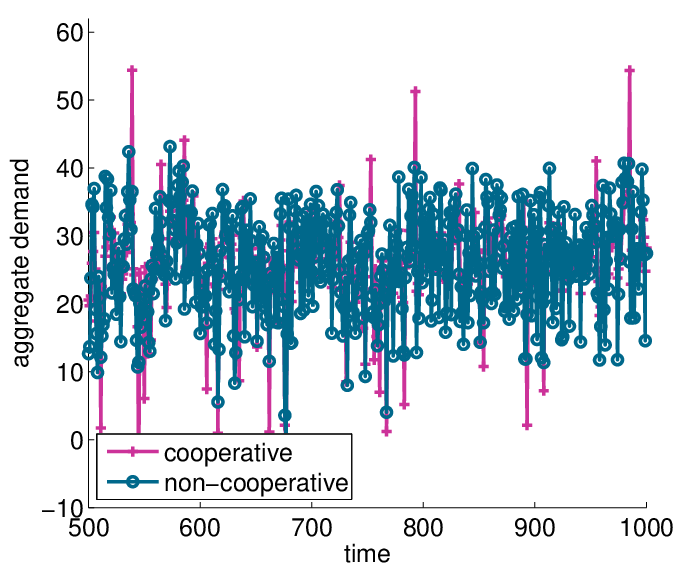
  Figure B.5 shows the sample paths of the aggregate demand process under the non-cooperative and the cooperative market architecture. In Figure B.5(a), we observe that at a smaller time scale, the cooperative scheme can better smooth the aggregate demand process, which is consistent with the lower aggregate demand variance. However in Figure B.5(b), at a larger time scale, we can identify more demand spikes produced endogenously by the cooperative load scheduling scheme, corresponding to the higher risk of the cooperative scheme.

• •

  Figure B.6 plots the empirical distributions of the aggregate demand process in both linear scale in Figure B.6(a) and in log scale in Figure B.6(b). We observe that under the cooperative market architecture, the distribution is more concentrated around the mean. However, associated with a higher risk, the distribution also has a heavier tail when compared to that in the non-cooperative scheme.

  Figure B.12 shows the resulting aggregate demand stationary distribution of the cooperative and the non-cooperative load scheduling scheme under the non-negative demand constraint. We observes that it qualitatively resembles the corresponding distribution Figure B.6 in most essential aspects.

We also point out that the tradeoffs we observed hold not only between the cooperative and non-cooperative market architectures above, but also exist in a variety of oligopolistic market architectures. Even when the agents can coordinate their actions and are risk sensitive, so that large spikes are mitigated, the tradeoff still exists and is shaped by different market achitectural properties. In Appendix D.1, we provide two parameterized variations of the market architectures, where the number of new arrival of each type can be great than 1, and where the agents can be risk sensitive, seperately.

References

- [1] R. Belhomme, R.C.R. De Asua, G. Valtorta, A. Paice, F. Bouffard, R. Rooth, and A. Losi. Address-active demand for the smart grids of the future. In SmartGrids for Distribution, 2008. IET-CIRED. CIRED Seminar, pages 1–4. IET, 2008.
- [2] D.P. Bertsekas. Dynamic programming and optimal control 3rd edition, volume ii. 2011.
- [3] R. Buyya and M. Murshed. A deadline and budget constrained cost-time optimisation algorithm for scheduling task farming applications on global grids. Arxiv preprint cs/0203020, 2002.
- [4] R. Buyya, C.S. Yeo, and S. Venugopal. Market-oriented cloud computing: Vision, hype, and reality for delivering it services as computing utilities. In High Performance Computing and Communications, 2008. HPCC’08. 10th IEEE International Conference on, pages 5–13. Ieee, 2008.
- [5] J. Chae. Trading volume, information asymmetry, and timing information. The Journal of Finance, 60(1):413–442, 2005.
- [6] A.I. Cohen and C.C. Wang. An optimization method for load management scheduling. Power Systems, IEEE Transactions on, 3(2):612–618, 1988.
- [7] Romain Couillet, Samir Medina Perlaza, Hamidou Tembine, and Mérouane Debbah. A mean field game analysis of electric vehicles in the smart grid. In Computer Communications Workshops (INFOCOM WKSHPS), 2012 IEEE Conference on, pages 79–84. IEEE, 2012.
- [8] J. Danielsson and H.S. Shin. Endogenous risk. Modern risk management: A history, pages 297–316, 2003.
- [9] J. Danielsson, H.S. Shin, and J.P. Zigrand. Endogenous and systemic risk, 2011.
- [10] J.M. Foster and M.C. Caramanis. Energy reserves and clearing in stochastic power markets: The case of plug-in-hybrid electric vehicle battery charging. In Decision and Control (CDC), 2010 49th IEEE Conference on, pages 1037–1044. IEEE, 2010.
- [11] J. Geanakoplos. The leverage cycle. Yale University, Cowles Foundation for Research in Economics, 2009.
- [12] E.J. Green. Non-cooperative price taking in large dynamic markets. Econometric Research Program, Princeton University, 1978.
- [13] S.J. Grossman and J.E. Stiglitz. On the impossibility of informationally efficient markets. The American Economic Review, 70(3):393–408, 1980.
- [14] L.P. Hansen and T.J. Sargent. Discounted linear exponential quadratic gaussian control. Automatic Control, IEEE Transactions on, 40(5):968–971, 1995.
- [15] T.T. Kim and H.V. Poor. Scheduling power consumption with price uncertainty. Smart Grid, IEEE Transactions on, 2(3):519–527, 2011.
- [16] W. Leontief. Stackelberg on monopolistic competition. The Journal of Political Economy, 44(4):554–559, 1936.
- [17] C. Li and L. Li. Utility-based scheduling for grid computing under constraints of energy budget and deadline. Computer Standards & Interfaces, 31(6):1131–1142, 2009.
- [18] E. Maskin and J. Tirole. A theory of dynamic oligopoly, iii: Cournot competition. European Economic Review, 31(4):947–968, 1987.
- [19] E. Maskin and J. Tirole. A theory of dynamic oligopoly, i and ii. Econometrica: Journal of the Econometric Society, pages 549–569, 1988.
- [20] A.H. Mohsenian-Rad and A. Leon-Garcia. Optimal residential load control with price prediction in real-time electricity pricing environments. Smart Grid, IEEE Transactions on, 1(2):120–133, 2010.
- [21] C. Nottola, F. Leroy, and F. Davalo. Dynamics of artificial markets. In Toward a practice of autonomous systems: proceedings of the First European Conference on Artifical Life, page 185. MIT Press, 1994.
- [22] M. Roozbehani, M.I. Ohannessian, M. Donatello, and M.A. Dahleh. Load-shifting under perfect and partial information: Models, robust policies, and economic value. Submitted to Operations Research.
- [23] F.C. Schweppe. Spot pricing of electricity. Springer, 1988.
- [24] L.S. Shapley. Stochastic games. Proceedings of the National Academy of Sciences of the United States of America, 39(10):1095, 1953.
- [25] R.A. Stubbs and D. Vandenbussche. Multi-portfolio optimization and fairness in allocation of trades. 2009.
- [26] P. Whittle and P.R. Whittle. Risk-sensitive optimal control. Wiley Chichester, 1990.