Bound states for the quantum dipole moment in two dimensions
Abstract
We calculate accurate eigenvalues and eigenfunctions of the Schrödinger equation for a two-dimensional quantum dipole. This model proved useful for the study of elastic effects of a single edge dislocation. We show that the Rayleigh-Ritz variational method with a basis set of Slater-type functions is considerably more efficient than the same approach with the basis set of point-spectrum eigenfunctions of the two-dimensional hydrogen atom used in earlier calculations.
1 Introduction
In a recent paper Dasbiswas et al[1] discussed the bound-state spectrum for a straight edge dislocation oriented along the axis. Within the continuum model, the authors reduced the problem to the two-dimensional Schrödinger equation for a quantum dipole. They obtained very accurate eigenvalues and eigenfunctions by means of a discretization of the space. Since this real-space diagonalization method (RSDM) is not so practical for highly excited states, those authors also carried out a Rayleigh-Ritz (RR) variational calculation with the basis set of eigenfunctions of the two-dimensional Coulomb problem[2].
The variational RR eigenvalues are known to approach the exact ones from above. However, in the present case the ground-state energy calculated with as many as basis functions exhibits a considerable discrepancy with respect to the same eigenvalue obtained by RSDM . Later on, Amore[3] carried out a more accurate calculation with hydrogen eigenfunctions and obtained as well as by fitting and extrapolating the outcome of a Shanks transformation. The authors of both articles resorted to a variational parameter (decaying parameter[1] or length scale[3]) that considerably improves the result. The remaining disagreement between RR and RSDM is probably due to the well known fact that the basis set used in those calculations is not complete because it does not include the continuous spectrum[2] (see, for example Ref. [4] and the references therein). For this reason the RR calculation proposed by those authors[1, 3] is expected to have a limited accuracy no matter how large the dimension of the basis set of discrete states. It is surprising, however, that the lack of the continuous wavefunctions appears to be more noticeable for the ground state. In addition to it, at first sight it seems that there is a better agreement for the odd states[1].
The purpose of this paper is to carry out a RR calculation with a nonorthogonal basis set of square-integrable functions that in principle does not require the continuous spectrum. In section 2 we describe the RR variational method with such an improved basis set. In section 3 we compare present results with those obtained earlier by Dasbiswas et al[1] and Amore[3]. Finally, in section 4 we summarize the main results and draw conclusions.
2 Rayleigh-Ritz variational method
The linearized model for the Ginzburg-Landau theory leads to the Schrödinger equation
| (1) |
where , , and is the strength of the dipole potential[1]. Choosing the units of length and energy we obtain the dimensionless eigenvalue equation
| (2) |
where . Since the potential is invariant under reflection about the axis , then the wavefunctions are either even or odd under such coordinate transformation.
Dasbiswas et al[1] and Amore[3] resorted to the RR variational method with the basis set of eigenfunctions of the planar hydrogen atom:
| (3) |
where and is the normalized solution to the radial equation[2]. However this basis set is incomplete if one does not include the eigenfunctions for the continuous spectrum (see, for example,[4] and references therein).
If, on the other hand, the chosen basis set of square-integrable functions does not require the continuous spectrum to be complete then one expects the accuracy of the RR variational results to be determined only by the basis dimension. Here we propose the nonorthogonal set of functions
| (4) |
for the even states and
| (5) |
for the odd ones, where is a variational parameter. This basis set resembles the Slater orbitals commonly used in quantum chemistry calculations of atomic and molecular electronic structure[4].
The RR method with the variational ansatz
| (6) |
leads to the generalized eigenvalue problem
| (7) |
where and . Note that it is possible to obtain explicit expressions for both kinds of matrix elements in terms of the variational parameter ; even more important is the fact that, with the help of a computer algebra software, like Mathematica, we can obtain the inverse of explicitly for all the cases considered in the present paper. In this way the inversion does not introduce any round-off errors and the original generalized eigenvalue problem is converted to the ordinary eigenvalue problem
| (8) |
for the nonsymmetric matrix .
3 Results
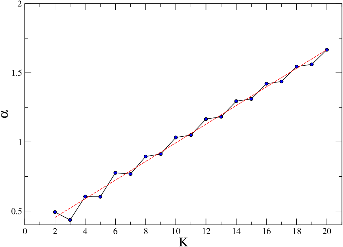
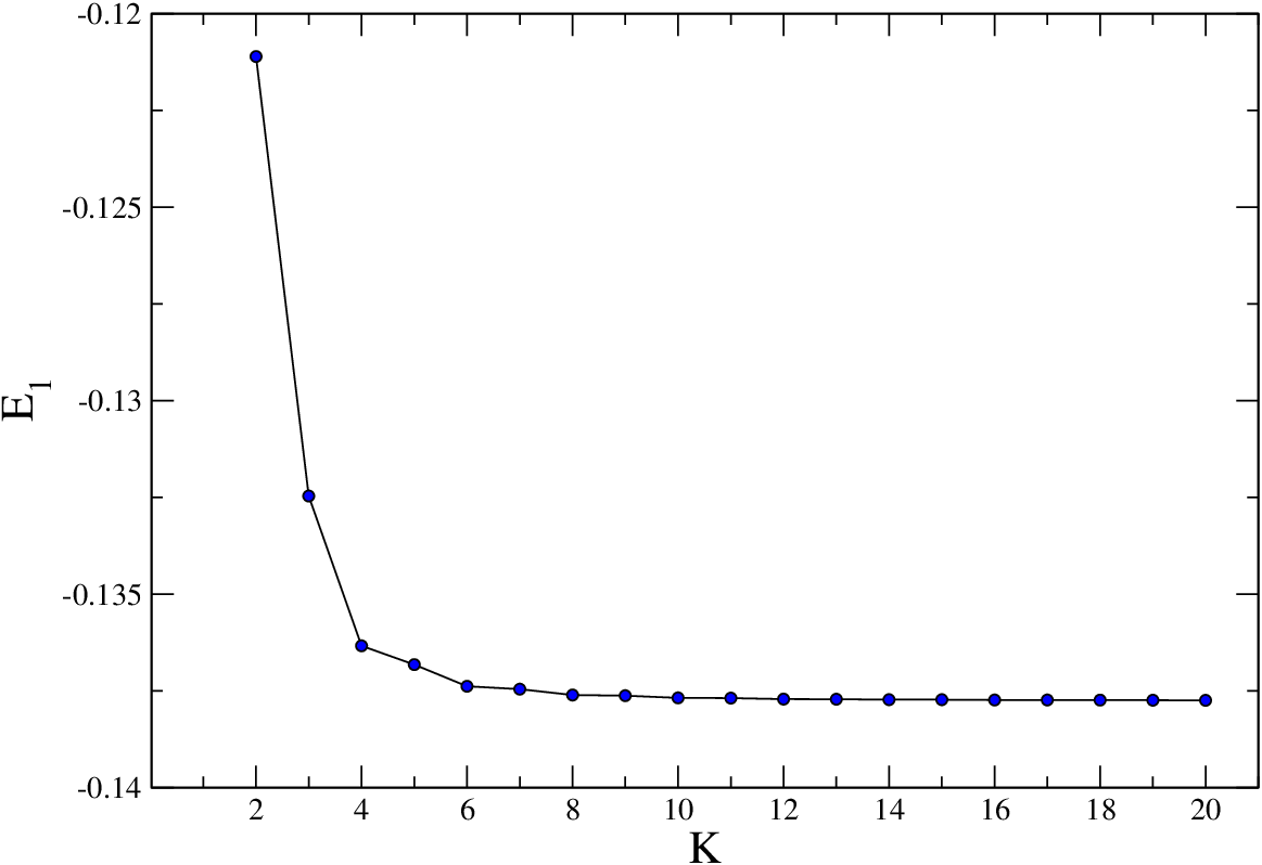
For brevity we write both the exact and approximate RR eigenvalues and eigenfunctions as and , respectively. We express the rate of convergence of the RR results in terms of the largest parameter in the wavefunction expansion (6), where and are the exponents of and in either equation (4) or (5). Thus, for a given value of there are basis functions of either even or odd symmetry. The optimal value of the nonlinear variational parameter depends on both the chosen eigenvalue and the number of terms in the wavefunction expansion (6). For example, Fig. 1 shows that for the ground state increases with oscillating about a straight line. Fig. 2 shows the RR eigenvalue for a range of values of . The rate of convergence is remarkably greater than the one for the Coulomb basis set[3].
Table 1 shows the RR eigenvalues obtained with the nonorthogonal basis sets (4) and (5) () on the one side and with the basis sets of even and odd Coulomb functions (3) () on the other. We appreciate the following facts: the accuracy of present nonlinear basis set is always greater () in spite of the fact that the RR calculations have been carried out with with nonorthogonal basis functions ( and Coulomb functions[3]. The discrepancy is greater for the lowest states and, it is less noticeable for the odd ones. We are presently unable to provide a rigorous proof for the last two facts; however, we may conjecture that the omitted continuous spectrum is not so relevant in those cases where there is agreement between the NB and CB variational results. The number of digits in the entries of this table is dictated by comparison purposes and does not reflect the estimated accuracy of the calculation.
Both the analytical calculation of the matrix elements and the analytical inversion of the matrix are time consuming but we do them only once for all the states. On the other hand, the optimization of the variational parameter for every state is a time consuming calculation that we should repeat several times. Earlier and present calculations suggest that the RR variational method is less efficient for the ground state. For this reason we have attempted variational calculations with considerably greater basis sets only for this state. For example, we have obtained with NB functions ( and with ones (). These results suggest that the first 6 digits remain stable and, consequently, that the RR calculation with the Slater-type basis functions does not appear to approach the RSDM results any more closely. However, it is worth noticing that present RR eigenvalues agree with the RSDM ones within the error estimated by Dasbiswas et al[1].
By means of the approximate ground-state wavefunction in terms of the Slater-like orbitals we have also calculated the effective dimensionless coupling constant[1]
| (9) |
Dasbiswas et al[1] obtained by means of a simple variational function constructed from the first three elements of the even nonorthogonal basis set (4): and by means of the RSDM. Amore[3] obtained by means of a reduced RR basis set of Coulomb functions (). Note that just NB functions yield the same result as Coulomb ones. The RR method with functions () of the basis set (4) yields that is quite close to the RSDM result.
Figures 3, 4 (left panels), 5 and 6 show the contour plots for for the first five even and odd states obtained by means of the NB functions. One clearly realizes that there are two types of nodal lines and that the energy depends differently on each of them. The right panels of Figures 3 and 4 show 3D plots of the probability densities of the first even and odd states.
4 Conclusions
Present results clearly show that the basis set of Slater-type orbitals is preferable to the Coulomb basis set. With just a few functions of the former set one obtains results that are considerably more accurate than those arising from much larger sets of the latter. As argued above, the reason is that any linear combination of discrete-spectrum Coulomb eigenfunctions is orthogonal to the continuous-spectrum eigenfunctions. On the other hand, no continuous-spectrum functions are required when using the Slater-type basis set. The contribution of the continuous spectrum appears to be more relevant for the lowest states and for the even ones. However, we have not proved that the RR variational method with the Slater-type functions converges towards the actual eigenvalues as increases. Present variational eigenvalues converge to limits that are slightly larger than the RSDM ones and we cannot safely state that all the stable digits of our results agree with those of the exact eigenvalues. Accurate lower bounds are required for that purpose and we have not yet been able to obtain them. In spite of this fact, it is encouraging that present RR results agree with the RSDM ones within the reported accuracy of the latter[1]. If, as argued by Dasbiswas et al[1], the RR variational method is more convenient than the RSDM for highly excited states, then present contribution is relevant because there is no doubt that the basis set proposed in this paper is preferable to the Coulomb one.
References
- [1] Dasbiswas K, Goswami D, Yoo C-D, and Dorsey A T 2010 Phys. Rev. B 81 064516.
- [2] Yang X L, Guo S H, Wong K W, and Ching W Y 1991 Phys. Rev. A 43 1186.
- [3] Amore P 2012 Cent. Eur. J. Phys. 10 96.
- [4] Calderini D, Cavalli S, ColettiI C, Grossi G, and Aquilanti V 2012 J. Chem. Sci. 124 187.
- [5] MacDonald J K M 1933 Phys. Rev. 43 830.
| 1 | 1.667 | -0.1377416 | -0.1279886 | 0.3984 | -0.0232932 | -0.0232932 |
|---|---|---|---|---|---|---|
| 2 | 0.7002 | -0.0411524 | -0.0394579 | 0.2469 | -0.0125862 | -0.0125862 |
| 3 | 0.4273 | -0.0199679 | -0.0193729 | 0.1773 | -0.0079918 | -0.00799186 |
| 4 | 0.2676 | -0.0118525 | -0.0115734 | 0.1239 | -0.0055643 | -0.00556435 |
| 5 | 0.1515 | -0.0097472 | -0.0097472 | 0.0997 | -0.0053312 | -0.00533116 |