The Degrees of Freedom Region of the MIMO Interference Channel with Hybrid CSIT
Abstract
The degrees of freedom (DoF) region of the two-user MIMO (multiple-input multiple-output) interference channel is established under a new model termed as hybrid CSIT. In this model, one transmitter has delayed channel state information (CSI) and the other transmitter has instantaneous CSIT, of incoming channel matrices at the respective unpaired receivers, and neither transmitter has any knowledge of the incoming channel matrices of its respective paired receiver. The DoF region for hybrid CSIT, and consequently that of CSIT models, is completely characterized, and a new achievable scheme based on a combination of transmit beamforming and retrospective interference alignment is developed. Conditions are obtained on the numbers of antennas at each of the four terminals such that the DoF region under hybrid CSIT is equal to that under (a) global and instantaneous CSIT and (b) global and delayed CSIT, with the remaining cases resulting in a DoF region with hybrid CSIT that lies somewhere in between the DoF regions under the instantaneous and delayed CSIT settings. Further synergistic benefits accruing from switching between the two hybrid CSIT models are also explored.
Index Terms:
Channel state information, Degrees of freedom, Interference alignment, Interference channel, MIMO.I Introduction
The interference channel (IC) consists of two transmitters that communicate with their respective receivers in spite of the interference that each transmitter causes to its unpaired receiver. Because the exact capacity of the IC is still not known, investigation into the degrees of freedom (DoF), which is the pre-log factor of the capacity, has received considerable attention in recent years. For instance, under the assumption that the receivers have perfect knowledge of the channel matrices, the complete DoF region of the () MIMO Gaussian IC was characterized for the instantaneous CSIT setting in [1], for the no CSIT setting under the assumption on fading distributions that transmit directions at different receiver antennas are statistically indistinguishable in [2], [3, 4, 5], and for the delayed CSIT setting in [6].
This paper sheds light on the unexplored region between the instantaneous CSIT and delayed CSIT settings for the MIMO IC. It is not difficult to envisage a situation where the two transmitters have different types of CSI. For example, via feedback links, one transmitter has perfect and instantaneous CSIT corresponding to the incoming channels at a stationary receiver, while the other transmitter has only delayed CSIT corresponding to the incoming channels at a mobile receiver. We model such a combination of perfect and instantaneous CSIT at one transmitter and delayed CSIT at the other, under the name Hybrid CSIT.
We address some of the pertinent questions for such a model, especially the usefulness of providing perfect and instantaneous CSIT at one transmitter. To analyze the improvement in the DoF region over that of delayed CSIT accruing from this extra information, we first characterize the complete DoF region for the MIMO Gaussian IC under the hybrid CSIT model. Without loss of generality, we assume . When transmitter 1 has perfect and instantaneous CSIT of incoming channels at receiver 2, we call the model hybrid CSIT 1; and analogously hybrid CSIT 2 refers to the model where transmitter 2 has perfect and instantaneous CSIT of incoming channels at receiver 1. No channel state information at a transmitter is assumed of incoming channels at its paired receiver. The DoF regions for the two models are characterized separately.
To show the achievability of the DoF region, we develop a new two-phase achievability scheme. The instantaneous CSIT at one receiver is exploited for transmit beamforming in the null space of the unpaired receiver, thus nulling the interference at that receiver. Delayed CSIT at the other transmitter is used for retrospective interference alignment (RIA) in the second phase of the scheme. This combination of transmit beamforming and RIA allows us to take maximal advantage of both forms of CSIT.
The characterization of the DoF regions for the hybrid CSIT models allows us to compare delayed CSIT, hybrid CSIT 1 and 2 and perfect and instantaneous CSIT models. This yields the encouraging result that for a large number of cases, hybrid CSIT 1 achieves the DoF region for perfect and instantaneous CSIT. Even for those cases where it fails to achieve the instantaneous CSIT DoF region, hybrid CSIT 1 still manages to improve over delayed CSIT. The results for hybrid CSIT 2 are more sobering; with the exception of one case, the DoF region remains the same as that of delayed CSIT. But for the one remaining case, there is an improvement over delayed CSIT, and the DoF region lies between that of delayed CSIT and perfect and instantaneous CSIT. The intuition behind the differing behavior of the two models becomes clearer when we realize that hybrid CSIT 1 allows interference nulling at the more constrained receiver i.e., the one with fewer antennas, thus allowing much bigger gains from transmit beamforming.
In an attempt at classification of CSIT models for the 2-user MIMO IC, we introduce four other CSIT models, namely the weaker hybrid CSIT 1 and 2 and enhanced hybrid CSIT 1 and 2 models. The weaker hybrid CSIT models are similar to the corresponding hybrid CSIT models, with the singular exception that the transmitter with instantaneous CSIT has no knowledge of the direct channel of its unpaired receiver in the weaker hybrid CSIT model. In the enhanced hybrid CSIT models, the transmitter with the delayed information in the corresponding original hybrid CSIT model knows its own cross-channel with delay, and all other channels are known at all transmitters instantly. We prove that the DoF region obtained for each of the original hybrid CSIT models also characterizes completely the DoF region of a large class of CSIT models, ranging from the corresponding weaker hybrid CSIT model to the corresponding enhanced hybrid CSIT model. More precisely, allowing the CSIT for each channel at each transmitter to be in one of three states i.e., unknown, known with a delay or known instantaneously and perfectly, we demonstrate that the DoF regions found in this work for the hybrid CSIT models applies to a total of CSIT models.
The DoF tuple of was shown to be achievable for the 2-user multiple-input single-output (MISO) BC with hybrid CSIT in [7], when the transmitter had instantaneous CSIT about one receiver and delayed CSIT about the other receiver. The characterization of the DoF region of the 2-user MIMO BC under the hybrid CSIT model was done later in [8].
Although recent work in [9, 10, 11] has investigated so-called mixed CSIT models for the two-user MISO BC, its extension to the IC in [12] is fundamentally different from the hybrid CSIT models analyzed here. The mixed CSIT model for the IC in [12] applies to situations where each transmitter has the same mix of both delayed CSIT and an imperfect version of instantaneous CSIT. On the other hand, transmitters in the hybrid CSIT models are distinguishable by the fact that they incorporate the heterogeneity of terminals as it relates to their mobility, the capacity of their feedback links, etc., resulting in the knowledge of channels being different at the two transmitters. The focus in this paper is on having delayed CSIT at one transmitter and instantaneous CSIT at the other regarding the cross links and the direct links of the unpaired receivers, with no CSIT at either transmitter of the cross and direct channels at its respective paired receiver. We note here again that for the two-user MISO BC, [11] establishes the DoF of the general mixed-CSIT model wherein the quality of current channel knowledge is different at the two transmitters which therefore also generalizes the work of [9, 10] as well as the DoF result for the hybrid CSIT model of [7].
It has also come to the attention of the authors after this work was posted on Arxiv ([13]) that [14] considers the so-called alternating CSIT model for the two-user multiple-input single-output (MISO) broadcast channel (BC) with a two-antenna transmitter and two single-antenna receivers, where the transmitter’s knowledge of the channels to the two receivers alternates between the various combinations of instantaneous, delayed and no CSIT (like the hybrid models of this work) and this variation of channel knowledge is shown to yield additional or synergistic DoF benefits. However, while [14] characterizes the DoF of the two-user MISO BC for the alternating CSIT model, this work characterizes the DoF of certain hybrid CSIT models for the two-user MIMO IC with an arbitrary number of antennas at each of the four nodes. Demonstration of such a synergistic benefit accrued by switching between the two hybrid CSIT models is also given. Extensions of achievable schemes in [14] from the 2-user MISO BC to the 2-user MISO IC are shown. The alternating CSIT model is further developed for the MIMO IC, with an example of an achievability scheme for the MIMO IC with synergistic benefits being illustrated.
The channel model is described in the next section, followed by main results in Section III. Section III also includes the proof of the outer bounds for the DoF region, as well as an extension of these outer bounds to a much larger class of CSIT models. A detailed example of the achievability scheme is also given in the same section, with a discussion about the range of CSIT models the achievability scheme applies to. Examples illustrating the extension of this achievability scheme into the realms of alternating CSIT are developed next. The generalized achievability scheme is given in Section IV, followed by detailed proofs of the optimality of the scheme in Section V. Conclusions can be found in Section VI.
II THE CHANNEL MODEL
In this section, we describe the ( MIMO interference channel (IC) under the assumption of hybrid CSIT. The channel consists of two transmitters and , with and antennas, respectively, and their paired receivers and , with and antennas, respectively. Without loss of generality, we assume that . Here, transmitter () has a message intended only for the receiver , but its transmit signal causes interference at the other receiver. At the channel use, signals received at the two receivers are given by
where is the transmitted signal from transmitter ; is the signal received by receiver ; is the additive noise at receiver ; is the channel matrix from Transmitter to Receiver ; and both transmitters have a power constraint of i.e
The channels are assumed to be Rayleigh faded, i.e., all entries of all matrices are independent and identically distributed (i.i.d.) zero-mean, unit-variance complex normal random variables. The additive Gaussian noise is similarly modeled as a complex normal random variable i.e., . Also, the channel matrices and the Gaussian noise are assumed to be i.i.d across time and independent of each other.
Both the receivers are assumed to have perfect and, without loss of generality, instantaneous knowledge of all channel matrices. In this paper, we investigate the DoF region when one transmitter has perfect and instantaneous CSIT, while the other transmitter has access only to delayed CSIT. More precisely, we study the situation where the channel matrices corresponding to one receiver are known at its unpaired transmitter perfectly and instantaneously, while the channel matrices corresponding to the other receiver are known to its unpaired transmitter with some finite delay, assumed without loss of generality and for convenience to be of 1 time slot. Such a situation, for instance, can be a consequence of differing mobility of the two receivers.
In hybrid CSIT 1, transmitter has perfect and instantaneous knowledge of channel matrices corresponding to receiver , while transmitter has delayed knowledge of the matrices corresponding to receiver . Moreover, transmitter has no knowledge of channels of receiver and transmitter has no knowledge of channels of receiver . In hybrid CSIT 2, transmitter has perfect and instantaneous knowledge of channel matrices corresponding to receiver while transmitter has delayed knowledge of corresponding to receiver . As in the case of the Hybrid CSIT 1 model, neither transmitter has knowledge of channels of its paired receiver. and refer to the DoF region for the hybrid CSIT 1 and hybrid CSIT 2 cases, respectively. Because of the assumption , the two cases are not symmetric and will need to be dealt with separately.


Knowledge of each of the four channel matrices and at each of the two transmitters can be in one of three states: unknown, known with a delay or known perfectly and instantaneously. Thus, there exist a total of possibilities for side information. Fortunately, not all these possibilities require individual attention. Indeed, it is shown in this work that the DoF region of the hybrid CSIT 1 model applies to side information models as does the DoF region of the hybrid CSIT 2 model. We note here that the DoF region obtained in [6] for the delayed CSIT model applies to possible side information models and the DoF region of the perfect and instantaneous CSIT model in [1] similarly applies to another side information models. Although a complete classification of all the models is not available at this time, this paper makes progress in that direction.
To illustrate the range of CSIT models to which the DoF regions obtained in this paper are applicable, we define four other CSIT models : enhanced hybrid CSIT 1 and 2 models, shown in Fig. 4 and 4, and weaker hybrid CSIT 1 and 2 models, shown in Fig. 6 and 6. In the weaker hybrid CSIT models, the transmitter with perfect and instantaneous CSIT does not know the direct channel of its unpaired receiver, and the knowledge about the rest of the channels at each receiver remains the same as in the respective original hybrid CSIT model. In the weaker hybrid CSIT 1 model, knows instantaneously the cross-channel matrix whereas has delayed knowledge of and . Similarly, in the weaker hybrid CSIT 2 model, knows instantaneously the cross-channel matrix whereas has delayed knowledge of and . In particular, has no knowledge of in the weaker hybrid CSIT 1 model and has no knowledge of in the weaker hybrid CSIT 2 model. In the enhanced hybrid CSIT 1 model, the cross-channel is known with a delay at and instantaneously at , and all other channels are known at both transmitters perfectly and instantaneously. Similarly, in the enhanced version of the hybrid CSIT 2 model, is known with a delay at and known instantaneously at , and all other channels are known at both receivers perfectly and instantaneously.
Let and be the two independent messages to be sent from to and to respectively. A rate tuple is said to be achievable if there exists a codeword spanning channel uses, with a power constraint of , such that the probability of error at both receivers goes to zero as , where . The capacity region of the IC is the region of all such achievable rate tuples, and the degree of freedom is defined as the pre-log factor of the capacity region i.e.,
| (1) |
The DoF region of various scenarios that are referred to in this paper are as follows:
-
Neither transmitter has any knowledge of channel realizations.
-
Both transmitters have delayed CSIT i.e., knows and knows , both with a delay. This DoF region has been characterized in [6].
-
has perfect and instantaneous knowledge of ; while has delayed CSI of .
-
has perfect and instantaneous knowledge of ; has delayed CSI of .
-
Both transmitters have perfect and instantaneous knowledge of the channel matrices of their unpaired receivers. This DoF region has been characterized in [1].
III Main Results
Definition 1.
For , Condition is said to hold, whenever the inequality
is true for with . The two conditions can not be true simultaneously, and are symmetric counterparts of each other. Also, condition can not hold if .
We list all the outer bounds from [6] that are applicable to the more constrained delayed CSIT case in inequalities 2-8.
| (2) | |||||
| (3) | |||||
| (4) | |||||
| (5) | |||||
| (6) | |||||
| (7) | |||||
| (8) |
Lemma 1.
The outer bounds and apply to the hybrid CSIT 1 model, while the outer bounds and apply to hybrid CSIT 2. The outer bounds hold for both hybrid CSIT 1 and CSIT 2 models.
Proof:
The outer bounds and have been proved for the delayed CSIT model in [6]. We first give a quick summary of the major elements of the proof of for the delayed CSIT model, before pointing out why and do not apply to the hybrid CSIT 1 model. In [6], under the assumption that does not face any interference, it was first shown that it is sufficient to consider only the first and antennas of and respectively (Lemmas 2 and 3 in [6]). The statistical equivalence of channel outputs was then established, which states that the signals received at any two antennas at time are statistically equivalent to each other, conditioned on the received outputs at previous times, knowledge of all present and past channels and the outputs at some other antennas at time (Lemma 4 and Remark 7 in [6]). These results were used to derive various inequalities involving the differential entropy of the signals at the two receivers, which were in turn employed to establish a lower bound on the DoF occupied by the interference at (Lemma 1 in [6]), which was shown to be proportional to . Finally, the outer bound for the delayed CSIT case was obtained from Fano’s inequality and the above mentioned lower bound on the interference DoF at . The outer bound for the delayed CSIT case was also proved using the same techniques involved in the proof , notably the statistical equivalence of channel outputs, but while accounting for the interference seen at both receivers.
A more detailed perusal of the proofs of and , in particular Lemma 4 in [6], shows that the statistical equivalence of two antennas is based on the transmit signal being independent of and (where and are arbitrary antennas of , while and are the and rows of matrix ), conditioned on a set of random variables that involve past channel outputs, present channel outputs at some other antennas and the previous channel matrices. This condition on is equivalent to the condition that does not know the channel instantaneously, ensuring that remains uncorrelated with and conditioned on the previous set of random variables. Thus, and do not apply to the hybrid CSIT 1 model, where has instantaneous knowledge of . On the other hand, the proofs for and in [6] , which are the same the proofs of and respectively, except for an exchange of roles between and , are verified to carry over for the hybrid CSIT 1 model. The analogous condition for the statistical equivalence of channel outputs to hold in this case is for not be known at instantaneously , a condition that is true for the hybrid CSIT 1 model. Thus and apply to the hybrid CSIT 1 model. Similar arguments show that and apply to the hybrid CSIT 2 model, while and do not.
Outer bound is proved in [1], where both transmitters have perfect and instantaneous CSIT. It therefore applies to both the hybrid CSIT models under consideration. and follow from the fact that the DoF of a point-to-point MIMO link is limited by the minimum number of transmit and receive antennas. Since bounds and hold for every case under consideration, they will not be explicitly mentioned in any of the proofs for convenience. ∎
Corollary 1.
The outer bounds and also apply to the enhanced hybrid CSIT 1 model and the outer bounds and also apply to the enhanced hybrid CSIT 2 model.
Proof:
The same argument as in Lemma 1 shows that the only condition needed for and to hold is for to have a delayed knowledge of , which is precisely the condition mentioned for the enhanced version of the hybrid CSIT 1 model. A similar argument shows that and apply to the corresponding enhanced version of the hybrid CSIT 2 model. Thus, the outer bounds derived here are applicable to a much larger class of CSIT models than the hybrid CSIT models.∎
Definition 2.
is defined as the region bounded by and . Similarly, is defined as the region bounded by and .
Theorem 1 (Hybrid CSIT 1).
The DoF region of the MIMO IC under the hybrid CSIT 1 model is equal to i.e., .
Proof:
Lemma 1 proves that the DoF region is outer bounded by i.e., . We now show that the region is achievable i.e., , and hence .
Motivated by the proof of Theorem 2 in [6], we start by enumerating all possible cases of the tuple in Table I. The cases are exhaustive and mutually exclusive. Except for the case (A.I.3b in Table I), we show that the DoF region for perfect and instantaneous CSIT is achievable even with hybrid CSIT 1, using techniques from [1] and [6]. This proves that , except when . A detailed case-by-case analysis of achievability is deferred to Section V.
| Case | Definition () | Active Bounds for Delayed CSIT (from [6]) | Hybrid CSIT 1 | Hybrid CSIT 2 |
| 0 | ||||
| Case A: and | ||||
| A.I | ||||
| 1 | ||||
| 2 | and | or | ||
| 3a | , and | |||
| 3b | , and | |||
| A.II | ||||
| Case B: and | ||||
| B | All cases | |||
and implicitly hold for every case under consideration.
For the remaining, and most interesting, case where ; we develop a new achievability scheme based on linear beamforming and retrospective interference alignment. This achievability scheme allows us to achieve the DoF region and hence is DoF-optimal. The details of the achievability scheme are described in Section IV. The key ideas behind the scheme are illustrated with an example in the next subsection. ∎
Theorem 2 (Hybrid CSIT 2).
The DoF region of the MIMO IC under the hybrid CSIT 2 model is equal to i.e., .
Proof:
Lemma 1 proves that the DoF region is outer bounded by i.e., . We now show that the region is achievable, which implies that , and hence .
All possible cases of the tuple are tabulated in Table I. Except for the case (A.I.3b in Table I), we show that the outer bound on the DoF region for hybrid CSIT 2 is the same as the DoF region for delayed CSIT i.e., . Since is already achievable with delayed CSIT achievability schemes from [6], this proves that is also achievable. Thus, , except for when . A detailed case-by-case analysis of achievability is deferred to Section V.
The achievability scheme developed previously in Theorem 1 can be easily adapted to the hybrid CSIT 2 model for the remaining case where . This achievability scheme allows us to achieve the DoF region and hence is DoF-optimal. As mentioned previously, the details of the achievability scheme are described in Section IV.∎
Corollary 2.
The achievability scheme developed here also applies to the weaker version of the hybrid CSIT models.
Proof:
We recall that the transmitter with perfect and instantaneous CSIT does not know the direct channel of its unpaired receiver in the weaker hybrid CSIT models. A careful perusal of the example given in III-A as well as the generalized alignment scheme in Section IV shows that for both the hybrid CSIT models, the transmitter with the perfect and instantaneous CSIT never needs to know the interference it creates (if any) at its unpaired receiver. For example, transmitter in hybrid CSIT 1 never needs to know any interference caused at . Hence, there is no necessity for that transmitter to know the incoming channels at its unpaired receiver, since its transmission scheme does not depend on this knowledge i.e., does not need to know for the hybrid CSIT 1 model. Thus, the achievability scheme applies to a weaker version of the hybrid CSIT models. ∎
Remark 1.
Corollaries 1 and 2 together establish that the DoF region characterized for each of the two hybrid CSIT models actually holds for a total of CSIT models. For example, provided is known perfectly and instantaneously at , is known with a delay at and is known either instantaneously or with a delay at , Corollaries 1 and 2 together imply that the DoF region remains the same as that of hybrid CSIT 1. Thus, CSIT about each of the channel matrices , and at and and at can be in one of three possible states i.e., not known, known with a delay or known instantaneously, without affecting the DoF region. These considerations, combined with the different CSIT states for at show that the total number of CSIT models for which the DoF region is completely characterized by the hybrid CSIT 1 DoF region is . Similarly, the DoF region for the hybrid CSIT 2 model characterizes completely the DoF regions for another CSIT models. Thus, this paper characterizes completely the DoF region of constituent CSIT models, out of a total of possible CSIT models.
Remark 2.
Of the constituent CSIT models for which the DoF regions are known, we note that [1], which obtains the DoF region for the perfect and global CSIT problem, actually characterizes the DoF region for constituent CSIT models. The achievability of the DoF region obtained therein applies to the case of side information corresponding to each transmitter knowing instantaneously the cross-channel into the unpaired receiver, with the knowledge about the rest of the channel matrices at each transmitter being in any one of three possible states i.e., not known, known with a delay or known instantaneously. This implies of course that the DoF region found in [1] for the perfect and global CSIT case where both transmitters know all four channel matrices instantaneously actually applies to a total of CSIT models. In the same vein, the DoF region for delayed CSIT in [6] applies for constituent CSIT models. For these constituent models, the DoF region is characterized by the cross-channels and being known with a delay at and respectively, and being known either with a delay or instantaneously at and respectively, and the rest of the channel matrices at each transmitter being in one of the three possible states, thus giving a total of constituent CSIT models.
III-A Example of Achievability Scheme
We present here an illustrative example of our achievable scheme for the specific case of . We consider the hybrid CSIT 1 model for this example. From Theorem 1, the shape of the DoF region for this choice of transmitter and receive antennas is shown in Fig. 7. It is clear that if we can achieve the DoF pair , then the complete DoF region can be achieved by time-sharing. To achieve this DoF pair, it is sufficient if sends data symbols (DS) to , and sends DSs to , over a total of time extensions. The example demonstrates how this DoF pair can be achieved over time slots, under hybrid CSIT 1. The DSs to be transmitted from are denoted as , and the DSs from are .
Phase 1
Since additive noise does not change the DoF region, we ignore it henceforth. We divide our scheme into two phases. In phase 1, uses all its antennas to send all the DSs it needs to send to . Since, in this example, has to send DSs and has antennas, phase 1 requires time slots to be able to send all of them. Thus, phase 1 lasts for time slots , and are transmitted by in bundles of DSs per time slot over phase 1, as seen in Fig. 7.
In the hybrid CSIT 1 model, has instantaneous knowledge of which allows it to do transmit beamforming in the null space of . is matrix and thus has a null space of dimension . sends DSs over this 2-dimensional null space during each time slot in phase . Thus, transmits at time , and at , in the null space of , as seen in Fig. 7. Evidently, these DSs cause no interference at .
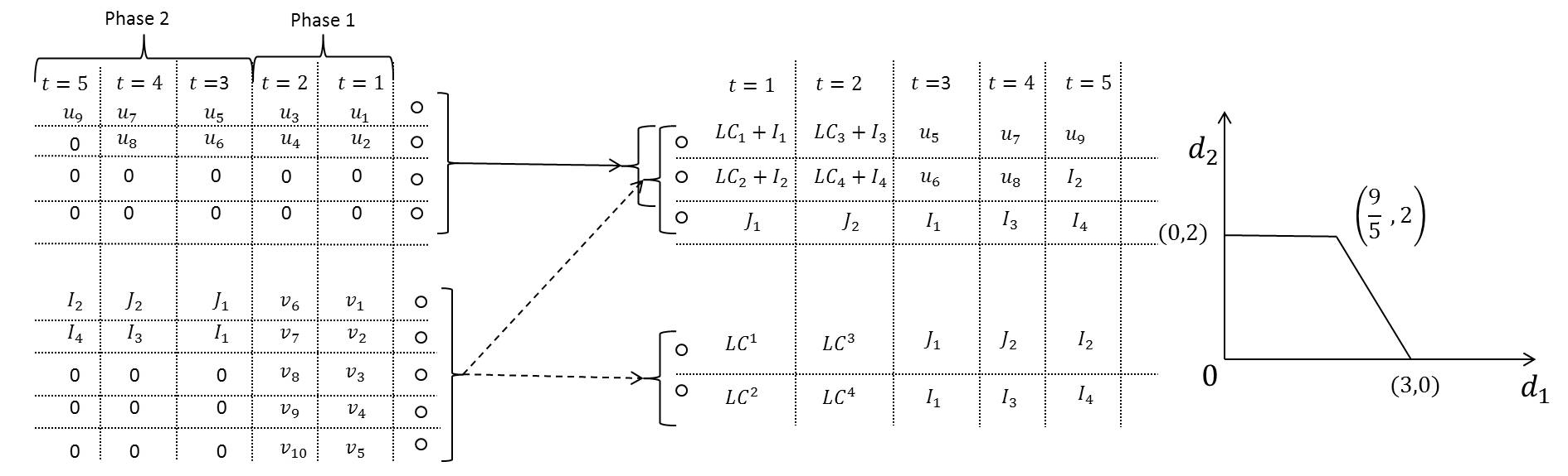
Knowledge of at permits it to calculate a unitary transformation matrix which allows to do receive beam-forming. This receive beamforming is done such that the DSs sent from affect only the first antennas of , or in other words, the last row of has all zeros. Over each time slot in phase 1, sees two linear combinations of the DSs transmitted from at its first two antennas, combined with interference from . The third antenna sees only interference from . For example, in time slot , the first two antennas of see linear combinations and of and , respectively, combined with interference and . The third antenna now sees interference . We note that the interference at e.g., , and at are linear combinations of DSs , in this case , intended for .
As already stated, sees no interference because of transmit beamforming at . Thus, in phase 1, obtains two linear combinations (of ) denoted as and at and two linear combinations (of ) denoted as and at . Since all the channel matrices are Rayleigh faded and can be shown to be full-rank almost surely, all the linear combinations and interference symbols found at both the receivers are linearly independent with probability . At the end of phase 1, none of the receivers is able to decode its intended data symbols. has only linear combinations available of its intended DSs. is not able to decode the linear combinations of its desired symbols , since they are combined with interference , respectively, but is able to learn the interference symbols and .
Phase 2
The objective of phase 2 is three-fold, (i) to provide sufficient number of independent linear combinations of at so that it is able to decode all its intended DSs, (ii) to transmit the remaining DSs from and (iii) to provide the interference symbols at , which would allow it to cancel the interference and thereby access the linear combinations . In phase 2, has (delayed) knowledge of channel matrices from phase 1, and also consequently of the transformation matrices . This allows to calculate all the interference caused at in phase 1, namely and . Now, if we can provide these symbols to , it will be possible for to decode all its intended DSs. Also, as mentioned earlier, knowledge of is useful at allowing it to cancel interference from phase 1. The interference symbols and are already known at , and it can simply cancel them out from its received signal. In other words, the interfering symbols and are retrospectively aligned with the interference from phase 1 at .
At time slot transmits and , while transmits again in the null-space of . Since sees no interference from , it is able to determine both and . Receiver cancels outs the already known , and after using a unitary transformation, is able to determine as well as its desired DSs and . It then cancels out from the combination received at time , to obtain the linear combination . The same strategy is again used at time , where transmits and and transmits . obtains , and , and uses to cancel interference from it obtained at and thus learn .
At , needs to transmit only , which it again transmits in the null space of . transmits the remaining interference symbols and . uses a unitary transformation such that only its first antenna is affected by . It uses the remaining two antennas to decode the two symbols and , which it then cancels from its received signals obtained in Phase to obtain , and . Thus, at the end of phase 2, has independent linear combinations of and the DSs , and thus can decode all its intended data symbols. Similarly, has linear combinations of , namely , , , and and five linear combinations of , namely , , , and . Hence can decode all its desired data symbols . The complete transmission scheme is clearly illustrated in Fig. 7.
Remark 3.
The careful reader will have noticed that although has (instantaneous) knowledge of the direct channel to its unpaired receiver i.e., , it never actually uses this information. The same holds true for the generalized achievability scheme in Section IV, which makes the achievability scheme developed here also applicable to the weaker version of the hybrid CSIT models.
Remark 4.
The final two columns of Table I give a concise comparison of the DoF regions for delayed CSIT, hybrid CSIT 1 and 2, and perfect and instantaneous CSIT. We notice that, except for the case , hybrid CSIT 1 achieves the DoF region for perfect and instantaneous CSIT and the DoF region for hybrid CSIT 2 is the same as that of delayed CSIT. It is only for the Case A.I.3b in Table I, i.e., that we observe the DoF region for both the hybrid CSIT models lying between the DoF region with only delayed CSIT and the DoF region with perfect and instantaneous CSIT. For the MIMO IC example used earlier in this Section, after fixing , we can achieve the DoF tuple with perfect and instantaneous CSIT, but only DoF with delayed CSIT (although the corner point is also achievable with delayed CSIT), and we recall that we were able to achieve DoF with hybrid CSIT 1. The difference between the DoF regions of the two hybrid CSIT models can be explained by the fact that transmit beamforming in hybrid CSIT 1 allows the interference to be zero-forced at , which being the receiver with the fewer antennas is more constrained than . This allows hybrid CSIT 1 to use its instantaneous CSIT for a greater gain.
III-B An Alternating CSIT Example
The alternating CSIT model allows for the CSIT configuration to change between time slots e.g., between hybrid CSIT 1 and hybrid CSIT 2. All the achievability schemes presented in [14] for the 2-user MISO BC can be adapted to the 2-user MISO IC, where each transmitter has 2 antennas and each receiver has a single antenna. The possible CSIT states in the MISO BC are mapped into the CSIT states of the MISO IC as follows: CSIT at about the cross-channel to in the IC is the same as the CSIT about the channel to receiver 1 in the BC, and similarly, CSIT about the channel to receiver 2 in the BC corresponds to CSIT at about the cross-channel to , with neither transmitter having any knowledge about the rest of the channels. Here, we further develop the alternating CSIT model for the 2-user MIMO IC in this example, elaborating a scheme that improves on the -MIMO IC hybrid CSIT 1 example given previously.
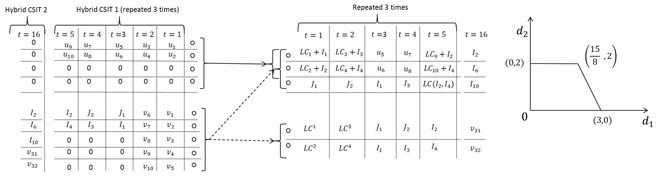
We use the freedom of alternating between the two hybrid CSIT models and the synergistic gains thus obtained to demonstrate the achievability of the DoF pair for the same IC of Section IV. We note that the DoF pair achieved with alternating CSIT is strictly better than the DoF tuple achievable with just hybrid CSIT 1 and the DoF tuples and achievable with only hybrid CSIT 2. To achieve this DoF pair, it is sufficient for to send DSs to and to send DSs to over time extensions. We do this by using the hybrid CSIT 1 model for the first time slots, and shifting to hybrid CSIT 2 for the last time slot. The DSs to be transmitted from are denoted as and the DSs transmitted from are denoted as .
Hybrid CSIT 1 Phase
We ignore the additive noise henceforth, since it does not affect the DoF region. We divide the total of 15 times slots with hybrid CSIT 1 into similar phases of time slots each, and depict one of these phases in Fig. 8. Each of these phases is similar to the hybrid CSIT 1 example explained previously in Fig. 7, including an unitary matrix transformation at to restrict the effect of its desired DSs to only the first antennas. The difference lies in the time slot, where now sends DSs, and instead of a single DS. The transmission scheme for remains the same for the time slots. At the end of this phase, has 5 linear combinations of i.e., and and 5 linear combinations of , namely and , and is thus able to decode all its DSs . On the other hand, is unable to learn the interference and , and as a result it can not cancel the interference to decode all of its desired DSs . We also observe that knows one linear combination of and (at ), denoted as in Fig. 8, and thus can learn if it is provided with . This shall allow it to cancel all the interference from its received outputs at , and to obtain four linear combinations, namely of , two linear combinations of and the DSs ,which is sufficient information to decode all its desired DSs from this phase. For this reason, providing to shall be the goal of our hybrid CSIT 2 phase.
The above hybrid CSIT 1 phase is repeated times, for a total of time slots. In these time slots, transmits DSs while transmits DSs . , as explained in the previous paragraph, is able to decode its intended DSs . on the other hand, as seen in the first phase, is unable to learn the interference symbols (from phase 1), (from phase 2) and (from phase 3), and hence is unable to cancel out all the interference. But since it possesses linear combinations , and , at the end of each of the three phases respectively, knowledge of and will allow it to determine the remaining interference symbols , and . This, in turn, allows to strip off all the interference from its received outputs, as illustrated in the previous paragraph, to learn sufficient number of linear combinations to be able to decode all its desired DSs . Thus, the goal of the hybrid CSIT 2 phase shall be to ensure that learns , and . In the same phase, also transmits two extra DSs and intended for receiver .
Hybrid CSIT 2 Phase
At time slot , we switch to the hybrid CSIT 2 model, where has perfect and instantaneous CSIT about . Since is a matrix, it has a dimensional null space. transmits DSs and in this null space, which are consequently not visible at . Along with and , also re-transmits and , having learnt these interference symbols in the hybrid CSIT 1 phases through delayed CSIT. does not transmit during this phase. Since has already knows and from the previous hybrid CSIT 1 phases, it is able to decode the two intended DSs and , which gives a total of DSs in time slots for . Receiver , which does not see and because of the aforementioned transmit beamforming at , is able to learn the interference symbols and using its antennas, and uses these with its earlier knowledge of , and to learn the remaining interference symbols and . Now can cancel away all the interference symbols it has seen in the previous time slots, and thus obtains sufficient linear combinations of its desired DSs to decode at the end of time slots. Thus, at the conclusion of the hybrid CSIT 2 phase, we achieve the promised DoF pair, using alternating CSIT.
IV Achievability Scheme
In this section, we describe an achievability scheme for the MIMO IC, which is applicable for the case , for both hybrid CSIT models. The scheme is explained here in detail for hybrid CSIT 1. Since the same scheme is easily adapted for the hybrid CSIT 2 model by simply interchanging the roles played by the two transmitters, the details for hybrid CSIT 2 will not be mentioned explicitly.
The achievability scheme is a hybrid of transmit beamforming and retrospective interference alignment, and is denoted henceforth as (Hybrid Interference Alignment). It is a generalization of the example described in the previous section. An overview of the scheme is given below, with the full exposition following later in this section.
- 1.
is designed to transmit data symbols (DSs) by coding over time slots, thus achieving DoF pair. The scheme is divided into two phases, consisting of and time slots respectively.
- 2.
The first phase is designed such that is able to transmit all the DSs. At each time slot in the first phase, transmits DSs using all its transmit antennas, while transmits as many DSs as possible in the null space of the channel . Thus, transmit beamforming allows to null out all interference at the receiver .
- 3.
Receive beamforming allows receiver to separate out the interference from into two subsets, and . These two subsets correspond respectively to the subsets and from the example in Section III-A. is able to decode the interference symbols from , and hence can be used by for retrospective interference alignment in the next phase. The aim of the next phase is to provide at both receivers, and at receiver . We will see that this gives each receiver sufficiently many independent linear combinations to be able to decode all of its intended DSs.
- 4.
At each time slot in phase 2, transmits as much as possible in the null space of , while transmits a combination of symbols from and . As mentioned earlier, is retrospectively aligned with the interference already known at , and is easily canceled out. Thus, decodes the interference symbols , as a result of which the effects of interference are canceled out from its received signals in phase 1. This allows to isolate linear combinations of its intended DSs. is able to decode and , which are linear combinations of its intended DSs. As seen in the previous example, both receivers are finally able to decode all their intended DSs from these linear combinations.
The details of the alignment scheme are explained below.
Phase 1 We choose the number of time slots in
this phase such that all the needed DSs can be sent from
transmitter , using all antennas. In the same phase,
at each time slot , transmits
DSs, taking care to keep them all in the null space of .
Hence, these DSs create no interference at .
then calculates a unitary transformation matrix from its knowledge of such that the symbols from affect only the first antennas of . Such a unitary transformation always exists, being essentially a change of basis transformation into a new orthonormal basis such that the first basis vectors now span the dimensional received signal space at , and can be calculated using a singular value decomposition (see 7.4.3 in [15]). The antennas denote the coordinates of the received signal in this new basis, and hence only the first antennas have non-zero symbols after the unitary transformation . The interference at any antenna of in time slot is denoted as . Interference at multiple antennas, e.g., at all antennas from to at time is denoted as . We next divide the interference at into two parts.
, is the collection of all interfering symbols at that have to be learnt by in phase 2 to be able to decode the data symbols of phase . These interfering symbols will be known at in phase 2 because of delayed CSIT and will also help to decode its intended data symbols by providing extra linear combinations of the transmitted symbols. It is easily shown that all these interfering symbols are linearly independent almost surely.
is the interference at that must be learned only at in phase 2. Since these interfering symbols are already known at by the end of phase 1, retrospective interference alignment is possible in phase 2. knows these interfering symbols in phase 2 because of delayed CSIT.
Phase 2 The goals to be achieved at each transmitter/receiver in phase 2 are as follows:
-
sends new data symbols over phase 2. As much as possible, these should be sent in the null space of to minimize interference at . The symbols, at each time slot , that can not be sent in the null space will cause interference at . This gives rise to the constraint
(9) -
should be able to accommodate both the data symbols sent by as well as the interfering symbols sent by . The symbols from are already known and can be discarded. This gives rise to the constraint
(10) -
faces interference symbols from which it discards. must also be able to decode both and . This gives rise to the constraint
(11) -
must send both (which is needed at both and ) and (which aligns with interference already known at ). At any given time slot , transmits according to the following constraints, (i) no more than symbols are transmitted, which ensures that can decode the symbols after discarding the interference symbols and (ii) no more than elements of are sent, allowing to accommodate these symbols.
Thus, this achievability scheme can to send symbols for the over time slots, provided the constraints (9)- (11) are satisfied. We shall prove later in Section V-A that only Case A.I.3b from Table I requires our attention, and show that the achievability schemes for delayed CSIT and perfect and instantaneous CSIT suffice for the rest of the cases. We divide Case A.I.3b again into 3 mutually exclusive and exhaustive sub-cases, which are shown to have different DoF regions in Section V, which are defined below,
- Case
-
I: ,
- Case
-
II: , ,
- Case
-
III: ,
We next check if these constraints are satisfied for the above sub-cases.
CASE I The parameters for Case I are , and inequality (9) is now equivalent to which is true since is true under Case I. It is also easily verified that inequalities (10) and (11) hold (with equality) for the parameters of Case I as well.
CASE II The parameters for Case II are , for which inequality (9) is equivalent to which is true since is true under Case II. Similarly, it is easily verified that inequalities (10) and (11) hold (with equality) for the parameters of Case I as well.
CASE III The DoF region for Case III has two non-trivial corner points, of which the point is considered first. For this point, the parameters are . Choose such that all the empty dimensions at in phase 2 are utilized i.e., , and we thus obtain With these parameters, inequality (9) is equivalent to
which holds with equality for the corner point Case III. Inequalities (10) and (11) are similarly verified to hold (with equality) for this corner point.We now consider the non-trivial corner point of the DoF region under Case III i.e, , for which the parameters are . Inequality (9) is now equivalent to which is true. Similarly, inequalities (10) and (11) are easily verified to hold (with equality) for this corner point.
We find that all the constraints are satisfied, and thus the achievability scheme can accommodate all the possible sub-cases.
V Proofs of Main Results
V-A Proof of Theorem 1
Consider each of the sub-cases in Table I for the hybrid CSIT 1 model.
- 0
-
As seen in Table I, the only active outer bound for the delayed CSIT case is the perfect and instantaneous bound . This outer bound is achievable even with just delayed CSIT, and therefore we have .
- B
-
Since , there is no null space from transmitter to . This allows us to use the transmit beamforming achievability scheme from [1], for the case where both transmitters have perfect and instantaneous CSIT. is supposed to transmit in the null space of ; but since no such null space exists for this case, it does not matter for the scheme whether has knowledge of channel state or not. This allows us to achieve the complete DoF region for the perfect and instantaneous case with hybrid CSIT 1. Thus, .
- A.II
-
Since , we use the same argument as for case B to prove that .
- A.I.1
-
The only outer bound that holds in this case is The outer bound region is given in Fig. 10. It is clear that it can be easily achieved by simple zero-forcing at transmitter . Thus, .
- A.I.2
-
As calculated previously in the proof of Theorem 2, the outer bounds and coincide. This shows that the DoF region for this case is the same as , which is achievable even by the interference alignment scheme for delayed CSIT. Thus, .
- A.I.3a
-
We consider first the sub-case of A.I.3 where . Calculating the outer bounds, we see that and coincide and are given as The DoF outer bound region is given by Fig. 10. It is clear that this DoF region can be easily achieved by transmit beamforming in the null space of at transmitter . Hence, .

Figure 9: Case A.I.1 (Hybrid CSIT 1) 
Figure 10: Case A.I.3.a (Hybrid CSIT 1) - A.I.3b
-
We calculate the applicable outer bounds for this case namely when , which are
It is obvious that this is the DoF region that needs considerable attention. It is convenient to further sub-divide this case into various mutually exclusive and exhaustive sub-cases and consider each sub-case separately.
When , we can transmit at most with antennas without loss of DoF optimality and hence can always remove any extra antennas from without affecting the DoF region. Thus, we only need to address the sub-case where . The outer bounds now becomeThis again gives rise to various sub-cases, which are enumerated below.
Case I: Recall that under Case I, . The outer bounds in this case areWe find that the only active outer bound is , and the DoF outer bound region is shown in Fig. 12.
Case II: Recall that under Case II, , . The outer bounds in this case areNow, we find that is inactive if the following inequality holds
i.e., (12) in which case, the DoF outer bound region is again as shown in Fig. 12.
Case III: Recall that under Case III, , . This is the sub-case where both the bounds and are active. The condition for both the bounds to be active is(13) and the DoF outer bound region is shown in Fig. 12.

Figure 11: Case I and II (Hybrid CSIT 1) 
Figure 12: Case III (Hybrid CSIT 1)
V-B Proof of Theorem 2
Here, we analyze each of the sub-cases in Table I, for the hybrid CSIT 2 model.
- 0
-
Since the only active outer bound is the perfect and instantaneous bound , which is achievable even with delayed CSIT, we have .
- B
-
The DoF region for delayed CSIT is defined by outer bounds , by Lemma 1, which are also active for the hybrid CSIT 2 case . Since this region is achievable even under the more stringent delayed CSIT condition, we have the result .
- A.II
-
In this case, the DoF region with delayed CSIT is defined by the outer bounds , which are also active for the hybrid CSIT 2 case, by Lemma 1. Since this region is achievable even under the more stringent delayed CSIT condition, we have the result .
- A.I.1
-
In case A.I.1, the DoF region with delayed CSIT is defined by the outer bound , by Lemma 1, which is also applicable for the hybrid CSIT 2 case. Since this region is already achievable by the more stringent delayed CSIT condition, we have the result .
- A.I.2
-
In this case, we have the conditions and . The outer bounds and now coincide and become . As a result, the only active outer bound for delayed CSIT is , by Lemma 1, which is also active for the hybrid CSIT 2 case. Thus, by the same argument as for the previous cases, we have the result .
- A.I.3a
-
We consider first the sub-case of A.I.3 where . By the same argument as for case A.I.2, we have .
- A.I.3b
-
This interesting case is defined by . The relevant outer bounds are
When , we can at most transmit with antennas and hence can always remove any extra antennas from without affecting the DoF region. Thus, we only need to discuss the sub-case where . The outer bounds now become
This again gives rise to cases I, II and III, defined previously in Section V-A, which are analyzed below.
Case I: Recall that under Case I, . The outer bounds in this case areWe find that the only active outer bound is , and the DoF outer bound region is shown in Fig. 14.
Case II: Recall that under Case II, , . The outer bounds in this case areWe find that is inactive under this case. Hence, the DoF outer bound region is again as shown in Fig. 14.
Case III: Recall that under Case III, , . This is the sub-case where both the bounds and are active. Hence, the DoF outer bound region has the form given in Fig. 14.
Figure 13: Case I and II (Hybrid CSIT 2) 
Figure 14: Case III (Hybrid CSIT 2)
VI Conclusion
In this paper, we study hybrid CSIT models for the general 2-user interference channel, where it is assumed that one transmitter has perfect and instantaneous CSIT of the channels at its unpaired receiver while the other transmitter has delayed CSIT of the channels at its unpaired receiver, with no channel state information at either transmitter about the incoming channels at their respective paired receivers. We obtain both DoF outer bounds and inner bounds, while developing a new DoF-optimal interference alignment scheme tailored for the hybrid CSIT models. The inner and outer bounds are shown to coincide, and we are thus able to characterize the complete DoF regions for both the hybrid CSIT models. By demonstrating an achievable scheme that uses less information than in the nominal hybrid CSIT models and by establishing that the DoF outer bounds hold for enhanced MIMO ICs with more side information, we show that the DoF regions of the nominal hybrid CSIT models actually apply to a total of hybrid CSIT models. We also demonstrate synergistic benefits from switching between hybrid CSIT models by showcasing achievability schemes that switch between the two hybrid CSIT models and achieve DoF tuples beyond the DoF region of either hybrid CSIT model.
References
- [1] S. A. Jafar and M. J. Fakhereddin, “Degrees of freedom for the MIMO interference channel,” IEEE Trans. Inform. Th., vol. 53, no. 7, pp. 2637–2642, Jul. 2007.
- [2] C. Huang, S. A. Jafar, S. Shamai, and S. Vishwanath, “On degrees of freedom region of MIMO networks without channel state information at transmitters,” IEEE Trans. Inform. Th., vol. 58, no. 2, pp. 849–857, Feb. 2012.
- [3] C. S. Vaze and M. K. Varanasi, “The degrees of freedom regions of MIMO broadcast, interference, and cognitive radio channels with no CSIT,” IEEE Trans. Inform. Th., vol. 58, no. 8, pp. 5354–5374, Aug. 2012.
- [4] Y. Zhu and D. Guo, “The degrees of freedom of isotropic MIMO interference channels without state information at the transmitters,” IEEE Trans. Inform. Th., vol. 58, no. 1, pp. 341–352, Jan. 2012.
- [5] C. S. Vaze and M. K. Varanasi, “A new outer-bound via interference localization and the degrees of freedom regions of MIMO interference networks with no CSIT,” in print, IEEE Trans. Inform. Th., 2012. [Online]. Available: http://arxiv.org/abs/1105.6033.
- [6] ——, “The degrees of freedom region and interference alignment for the MIMO interference channel with delayed CSIT,” IEEE Trans. Inform. Th., vol. 58, no. 7, pp. 4396–4417, Jul. 2012.
- [7] H. Maleki, S. A. Jafar, and S. Shamai, “Retrospective interference alignment over interference networks,” J. Sel. Topics Signal Processing, vol. 6, no. 3, pp. 228–240, Mar. 2012.
- [8] R. Tandon, M. A. Maddah-Ali, A. Tulino, H. V. Poor, and S. Shamai, “On fading broadcast channels with partial channel state information at the transmitter,” in Wireless Communication Systems (ISWCS), 2012 International Symposium on, aug. 2012, pp. 1004 –1008.
- [9] T. Gou and S. Jafar, “Optimal use of current and outdated channel state information: Degrees of freedom of the MISO BC with Mixed CSIT,” Communications Letters, IEEE, vol. 16, no. 7, pp. 1084 –1087, Jul. 2012.
- [10] S. Yang, M. Kobayashi, D. Gesbert, and X. Yi, “Degrees of freedom of time correlated MISO broadcast channel with delayed CSIT,” submitted, IEEE Trans. Inform. Th., Mar. 2012. [Online]. Available: http://arxiv.org/abs/1203.2550.
- [11] J. Chen and P. Elia, “Degrees-of-freedom region of the MISO broadcast channel with general mixed-CSIT,” May 2012. [Online]. Available: http://arxiv.org/abs/1205.3474.
- [12] X. Yi, D. Gesbert, S. Yang, and M. Kobayashi, “The DoF region of the multiple-antenna time correlated interference channel with delayed CSIT,” submitted, IEEE Trans. Inform. Th., Apr. 2012. [Online]. Available: http://arxiv.org/abs/1204.3046.
- [13] K. Mohanty, C. S. Vaze, and M. K. Varanasi, “The degrees of freedom region for the MIMO interference channel with hybrid CSIT,” Sep. 2012. [Online]. Available: http://arxiv.org/abs/1209.0047.
- [14] R. Tandon, S. A. Jafar, S. Shamai, and H. V. Poor, “On the synergistic benefits of alternating CSIT for the MISO BC,” Aug. 2012. [Online]. Available: http://arxiv.org/abs/1208.5071.
- [15] R. A. Horn and C. R. Johnson, Matrix Analysis. Cambridge University Press, 1985.