Spectrums of Black Hole in de Sitter Spacetime with Highly Damped Quasinormal Modes: High Overtone Case
Abstract
Motivated by recent physical interpretation on quasinormal modes presented by Maggiore[1], the adiabatic quantity method given by Kunstatter[2] is used to calculate the spectrums of a non-extremal Schwarzschild de Sitter black hole in this paper, as well as electrically charged case. According to highly damped Konoplya and Zhidenko’s numerical observational results for high overtone modes[3], we found that the asymptotic non-flat spacetime structure leads two interesting facts as followings: (i) near inner event horizon, the area and entropy spectrums, which are given by , , are equally spaced accurately. (ii) However, near outer cosmological horizon the spectrums, which are in the form of , , are not markedly equidistant. Finally, we also discuss the electrically charged case and find the black holes in de Sitter spacetime have similar quantization behavior no matter with or without charge.
Keywords:
area and entropy spectrums; highly damped quasinormal modes; de Sitter spacetimepacs
04.70.Bw, 04.70.Dy, 04.62.+vI Introduction
Issue regarding black hole (BH) quantization problem has been intensively and extensively focused on. As early as the 1970s, Bekenstein conjectured that if the horizon area is an adiabatic invariant, the horizon area should have a discrete and equally spaced spectrum [4, 5, 6],
| (1) |
where is a dimensionless constant and is the Planck length. The gravitational units of and are adopted. It shows that any classical adiabatic invariant should be corresponded to a quantum entity with discrete spectrum according to the Ehrenfest principle. After that, many people have obtained the spectrums for various dynamical modes with various parameter including and [7, 8, 9, 10, 11, 12].
Since the quantization of BH is put forth, people find that the quasinormal modes (QNMs) has a very important place in Loop Quantum Gravity. Hod firstly observed that the spacing parameter could be determined by the high overtones quasinormal (QN) frequencies [13, 14]. Subsequently, Kunstatter suggested that the system adiabatic invariant should have a form of in which is system energy and is vibrational frequency [2]. It is interesting that if we choose the real part of QN frequencies and the ADM mass as the vibrational frequency and the system energy , Hod’s result is obtained naturally through Kunstatter method.
Recently, Maggiore considers above situations and proposes that the QN frequencies should be treated as the proper frequency of the equivalent harmonic oscillator [1]. The change of the mass of BH is given by where is identified with the change between adjacent physical frequencies () where is overtones number. According to the harmonic oscillator theory, the actual frequency is , rather than original . For the highly damping limit , one has a proper frequency .
Although the usual QNMs are important for observational aspect of gravitational waves phenomena, the high overtones QNMs are typically ignored because these relevant modes damped infinitely fast do not significantly contribute to the gravitational wave signal. However, since Hod opens a new era connecting BH quantization and QNMs, the highly damped QNMs () has been attracted more attentions. Motl subsequently presents these asymptotic QNMs in Ref.[15] by continued fractions methods assuming the gauge group of the theory to be SO(3) [16]. However, when the numerical method becomes more hard to solve. Hence, Motl-Neitzke developed the monodromy method by matching several poles in the plane which can calculate the highly damped QN frequencies for any static spacetime in principle [17].
On the other hands of this paper, more astronomical observations [18, 19] demonstrate us a nonzero cosmological constant for the expanded universe whose topology structure presents more like a de Sitter case (for the review see Refs.[20, 21]). Schwarzschild de Sitter (SdS) spacetime becomes more and more important in the gravity theory. Recently, more attentions are paid on the near extremal SdS BH in which the BH event horizon and the cosmological horizon are close to each other [23, 24, 25, 26, 22]. In 2003 [23], Cardoso-Lemos obtained their QN frequencies for various radiative fields including scalar perturbation, electromagnetic perturbation and gravitational perturbation by using Pshl-Teller potential with very large imaginary part [27]. Then this result [23] has been used to quantize the area and entropy of the near extremal SdS BH [28, 22]. In early Setare’s work [28], the real part of QN frequencies is considered to be a fundamental vibrational frequency for a BH of energy. The area spectrum of near extremal case above is where is dependent on the form of perturbations: namely for scalar or electromagnetic perturbations, for gravitational perturbation. In the recent work [22], Li-Xu-Lu (LXL) have used Maggiore’s physical interpretation of quasinormal modes and restudied this near extremal case. They found the area spectrum is and the entropy spectrum is which are independent of the form of perturbations. Comparing the near extremal case [28, 22] with other systems [1, 29, 2], one will find it is similar to the single horizon BH because the inner horizon and outer horizon are degenerate into a extremal single horizon case, similar to Schwarzschild case. So under the same Maggiore’s interpretation, the result of Ref.[22] is in agreement with the results of Schwarzschild BH [29]. However, as far as we known there is no work relevant to the quantization for the more general SdS spacetime with non extremal cosmological constant. So based on above situations including Maggiore’s interpretation and highly damped QNMs of SdS BH, we use Kunstatter method to calculate the spectrums of area and entropy for SdS BH.
II Highly damped quasinormal modes of Schwarzschild de Sitter black hole
The static spherically symmetric metric of SdS BH is given by
| (2) |
where lapse function is
| (3) |
is BH mass and is de Sitter curvature radius. The spacetime above is bounded by two horizons, namely, inner event horizon and outer cosmological horizon , which are listed as followings,
| (4) |
where with . The real solutions are accepted only if satisfies [30]. The lapse function (3), hereby, could be rewritten as,
| (5) |
where the negative parameter has no physical meaning.
Matching Eqs.(3) and (5), we can get the relationships of BH mass and de Sitter curvature radius as
| (6) | |||||
| (7) |
According to the variations of Eqs.(6) and (7), we have the formulas with respect to , and as,
| (8) |
Then, we need introduce the surface gravity and the tortoise coordinate in the following words. According to the definition of surface gravity
| (9) |
one can easily obtain its explicit forms
| (10) | |||||
| (11) |
where and are the surface gravity at and , respectively. Submitting Eqs.(10) and (11) into Eq.(8), we can find the relationship between and
| (12) |
Here “” denotes the inverse relation between and , which indicates when BH mass increases (), increases (), but decreases (). Here, it is convenient to use Eqs.(8) and (12) to calculate the spectrums of area and entropy.
Through the definition of tortoise coordinate shown by
| (13) |
we can get
| (14) |
By using above coordinate Eq.(14) the perturbation field equation of could be reduced to a form of Schrödinger wave-like equation as
| (15) |
where is the radial component and is potential given by
| (16) |
which dominates the evolution of field in SdS spacetime. One of outstanding characteristics of this potential is that when approaches two horizons, the potential goes exponentially to zero.
Based on the potential (15), various QNMs could be solved out by adding some special boundary conditions [31]. In the early studies on the aspect of perturbation focus mainly on the dynamics of radiative field such as two-dimensional toy models [32, 33, 34], radiative three time evolution epochs [35], radiative tails [36], degenerate special Nariai BH [37, 38, 39] and so on. In order to calculate the spectrums of area and entropy, the highly damped QNMs must be found from them. Fortunately, there is an available case could be used for the computation of these spectrums, namely the high overtone case which is observed not only by Konoplya-Zhidenko’s numerical observations in Ref.[3], but also by Cardoso-Natrio-Schiappa’s theoretical analysis in Ref.[40] as well as Choudhury-Padmanabhan’s work in Ref.[41].
The accurate high overtones numerical quasinormal modes have been obtained by Konoplya-Zhidenko (KZ) in Ref.[3] by using Leaver approach [16] and Nollert’s [42] techniques. One interesting phenomenon from these results is that the average value of spacing over sufficiently large number of modes equals event horizon surface gravity , which could be expressed mathematically as
| (17) |
This result is in agreement with the analytical results presented by Cardoso-Natrio-Schiappa in Ref.[40]. Simultaneously, Choudhury-Padmanabhan [41] also study the corresponding analytic analysis of level spacing of the QNM frequencies and provide a derivation of the imaginary parts of frequencies for the SdS spacetime by calculating the scattering amplitude in the first Born approximation. It is found that the numerical observations and theoretical analysis all strongly indicate the spacing of high overtone’s imaginary part is proportional to the surface gravity of inner event horizon, rather than the surface gravity of the cosmological horizon in the view of actual physics. Certainly, the situation “scattering off the cosmological horizon” can happen in mathematics, which can be found in the part of Appendix C in Ref.[41]. Here, we do not consider it.
III area and entropy spectrums for Non-extremal Schwarzschild de Sitter black hole
For a given system with energy , Kunstatter proposes the adiabatic invariant quantity should have a integral of vibrational frequency as [2]
| (18) |
where we adopt according to the first law of BH thermodynamics. Apparently, how to choose the frequency becomes the key to calculate the spectrums. In Hod’s early work [13, 14], the transition frequencies equal the classical oscillation frequencies for large quantum numbers according to Bohr’s correspondence principle. The highly damped BH oscillations frequencies have a very large imaginary part for . It indicates the effective relaxation time for BH returning to static state is arbitrarily small. The degraded rapidly QNMs should be treated as one type of quantum transition in which the transition frequency is the real part of in a natural way.
However, according to Maggiore’s interpretation of QNMs [1], the Black hole perturbations should be looked as the damped harmonic vibration. As a result, the real frequencies of the equivalent damped harmonic oscillators are rather than , where is the real part and is the image part of . For the long lived modes , the real frequencies become . Contrary to long lived case, the frequencies become for the highly excited modes . Then, we consider the transition from mode to mode for a non-extremal cosmological constant. Thus according to the numerical observations (17) the transition frequency is .
Submitting the surface gravity (10) into Eq.(18), we can get the Kunstatter’s adiabatical invariant shown as
| (19) |
According to the positive quantization numbers in Bohr-Sommerfeld condition, the adiabatic invariant quantity has to be adopted the absolute value of integral (18) to compute the area and entropy spectrums through Kunstatter method [2]. If we consider the expresses of inner horizon and outer horizon , i.e. Eq.(4), adiabatically invariant is presented in two forms as,
| (20) | |||||
| (21) |
The constants appeared in above formulas (20) and (21) could be assimilated into integral constants.
Hence, if the Bohr-Sommerfeld (BS) quantization condition is adopted, Eqs.(20) and (21) are rewritten as
| (22) | |||||
| (23) |
where and . By using the area formulas: and , the quantum areas of inner event horizon and outer cosmological horizon are written as
| (24) | |||||
| (25) |
which lead to the spacing of area spectrums shown by
| (26) | |||||
| (27) |
where is a correction term to the spacing shown by
| (28) |
The entropies and of horizons and are listed as,
| (29) | |||||
| (30) |
It is interesting that the spectrums of area and entropy are equally spaced near inner event horizon. However, the spectrums are not equidistant near outer cosmological horizon.
Then, we have a look at the near extremal degenerate situation where is very close to . Mathematically, this limit case is corresponding to the specific parameters: and which lead the limits of and ,
| (31) |
Submitting Eq.(31) into above Eqs.(20) and (21), we can obtain
| (32) |
The quantum areas of horizons and are given by
| (33) |
The entropies also reduce to
| (34) |
It is clear that Eqs.(33) and (34) are exactly accordance with LXL’s results appeared in Ref.[22].
So according to the accurate high overtones numerical quasinormal modes observations (17), the area and entropy spectrums (, ), (, ) are obtained at event horizon and cosmological horizon , respectively. For the non-extremal SdS BH, (, ) are equally spaced near and (, ) are not marked equidistant. However, for the near-extremal SdS BH, the horizons and coincide and the area and entropy spectrums (, ) and (, ) are reduced to the same forms with equally spacing, namely Eqs.(33) and (34). In the SdS BH case, we find the behavior of QNMs frequency decides the results of area and entropy spectrums. For the very high overtones numerical quasinormal modes, the spacing of frequency is proportional to the surface gravity of event horizon , and not . Hence, this fact determinate the spacing of area and entropy spectrums is constant at event horizon , and is changed at cosmological horizon .
At the last part of this section, we need to analyse the not equidistant area spectrums of cosmological horizon . According to the based expressions Eq.(25), we can get
| (35) |
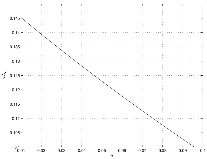
In order to observe the variation of spacing with and more clearly, we plot two figures below, one is vs in Fig.1 and another is vs in Fig.2. In the Fig.1, we fix the cosmological constant and draw the spacing of cosmological horizon area versus quantum number , which illustrates that decreases with increasing . At the same time, in the Fig.2, we fix the quantum number and draw the spacing of cosmological horizon area versus cosmological constant , which illustrates that also decreases with increasing .

At the end, it is well known that in the de Sitter spacetime another important type black hole contained electrically charge is the Reissner Nordstrm de Sitter black hole. One natural question is whether the behavior of above quantization of SdS BH is still valid for the electrically charged case. So we study this subject in the next section.
IV More General Setting: Electrically Charged Case
For a more rounded consideration, we expand the situation from no electrically charged SdS case to electrically charged case in this section. Based on the QNMs analysis [43, 24, 44], we investigate the quantization of Reissner Nordstrm de Sitter black hole (RNdS BH). In the relevant QNMs analysis, it is found that there is a great deal of observational evidence for the existence fact that the influence of charge on field propagation is mild, such as the constant tail for scalar perturbations with [35, 36, 43], the range of variation of the quasinormal modes [43], the exponential coefficients of exponential late time tail decay [43] and so on.
For RNdS BH the function is given by
| (36) |
Unlike the SdS case, there are three horizons: Cauchy horizon , event horizon and cosmological horizon in this spacetime with relationship . It should noticed that the results Eqs.(6) and (7) only hold for SdS case, for the RNdS case the Eqs.(6) and (7) are replaced by
| (37) |
where with no actual physical meaning.
According to the definition of surface gravity Eq.(9), we can get the corresponding surface gravities , to the horizons and shown by,
| (38) | |||||
| (39) |
Matching Eqs.(37) and (36), the relationships of , and are obtained as,
| (40) | |||||
| (41) | |||||
| (42) |
It is found that if the charge vanish , we can get according to Eq.(42). Hence, the relationships above reduce to the case of SdS, namely the Eqs.(6) and (7). Implementing the variation of Eqs.(40) and (42), we can get
| (43) |
Then submitting the Eq.(42) into Eq.(43), the relationship of , , are reduced to,
| (44) |
Submitting Eqs.(38) and (39) into Eq.(44), we can get a simple and important formulas as
| (45) |
where “” means that when increases will be decreased. It is noticed that the relationship above is obtained without any extremal assumption. Comparing with that of no-charge case it is easy to find this similar relationship about horizons and black hole mass could be also obtained in the SdS black hole case. In another words, the charge of black hole does not affect the quantization progress of black hole under de Sitter space-time. In spite of that we still need to finish the quantization of black hole contained charge in de Sitter space-time.
Then, we need to find the quasinormal frequencies which could be used calculate the area spectrums. Just like the words said by Ref.[24], it is usually difficult to calculate the analytic expressions for the quasinormal frequencies, except in particular situations. Here, we must face one difficulty of that there are not clear analytic expressions about RNdS black hole quasinormal frequencies, except the near extreme limit case [24, 43]. Unlike the SdS case, there are neither purely electromagnetic nor gravitational modes. Hence, four mixed electromagnetic and gravitational fields, two of them named polar fields, and , which impart no rotation to the black hole. And the last two are called axial fields, and . The deduction can be found in Refs.[45, 43, 24] and references therein.
The frequencies of quasinormal modes associated with the Pöschl-Teller potential are shown by [43]
| (46) |
The constant is denoted by for scalar perturbation , or for axial perturbations , or for polar perturbations . For the scalar field, is given by,
| (47) |
For the two axial potentials, and are given by,
| (48) | |||||
| (49) |
where
| (50) |
For the two polar potentials, and are given by,
| (51) | |||||
| (52) |
where and .
Then in the last words of this part we use the analytic QNMs frequencies (46) to derive the area spectrums of Reissner-Nordstrm-de Sitter black hole. For the highly excited black hole, the proper frequency adopts with very large . Hence, according to the former QNMs frequency (46), we can know that when the system transit from to the absorbed energy is
| (53) |
which also can be treated as the transition frequency.
Submitting above Eq.(53) into Eq.(18), we can get the adiabatic invariant in the form shown by,
| (54) |
Based on the Bohr-Sommerfeld condition, Eq.(54) leads directly the equally spaced mass spectrum as
| (55) |
The areas of horizons and are given by
| (56) |
The corresponding variations are given by
| (57) |
By using the former Eqs.(45), the above variations and is given by,
| (58) |
where . Clearly the area spectra of event horizon is equally spaced. Then we have a look at the cosmological horizon area , for the general case the ratio is not constant, the spaced of is not equally. However, for the near extremal RNdS black hole the three hypes of extremal horizons coincide, namely , we can get . And . It is observed that the influence of the no trivial electric charge is mild. The variation of area or entropy spectrums with the charge is not very large. In another words, the charge doses having no significant effect on the quantization of black hole in de Sitter background. This type behavior of quantization is agreement with the near extremal SdS black hole case [22]. In fact, if the formula (17) can be expanded to the all high overtones no matter with charge or without charge for the black hole in de Sitter background, the spectrums of area or entropy near event horizon are equally spaced accurately, but they are not markedly equidistant at cosmological horizon. However, for the near extremal black hole in which the horizons coincide each other, all area spectrums are equally spaced.
V Conclusion
In this paper, we have calculated the spectrums of non-extremal SdS BH by using Kunstatter method under Maggiore’s interpretation of QNMs. We summarize what has been achieved.
1. The QNMs plays a important role in the quest for a quantum gravity theory. The quantization of single horizon spacetimes has been attracted many people focused on including the Schwarzschild BH [13, 14, 2, 1, 29], non-rotating or rotating BTZ BH [29, 46], higher dimensional BH [2, 29]. However, few works address the nontrivial multi-horizons spacetime in non-asymptotically flat spacetime. Even for the near extremal SdS BH [22], the close inner and outer horizons situation leads to a usual processing method like single horizon case. It is highly necessary to investigate the area and entropy spectrums for non-asymptotically flat SdS BH with double horizons. Hence, we perform our calculation through Konoplys-Zhidenko’s result [3].
2. The spectrums of area and entropy are obtained by using Konoplys and Zhidenko’s QNMs [3]. The sum formula Eq.(17) reveals the statistic treatment on the average high overtone number . For the gravitational perturbations case, the spacing between nearby overtones shows peculiar periodic dependence on (illustrating in Fig. 4 of Ref.[3] where should be changed to ). But, the average value of these spacing over very large number of modes equals to the surface gravity at cosmological horizon . Hence, in the statistical viewing, the spacing of nearby overtones Eq.(17) is effective when overtone number is sufficiently large. For the electromagnetic perturbations, the spacing of damps to a equidistant spectrum for the very high , i.e. . Then, by using high overtones results Eq.(17) above, we naturally obtain the area spectrums (24) and (25) near event horizon and cosmological horizon , respectively. Through the area spectrum formulas proposed by Kunstatter’s [2], we find only the spectrum of inner event horizon is equally spaced.
3. In the last part of our calculation, we expand the quantization from the no charged black hole (SdS BH) to the charged black hole (RNdS BH). After our carefully calculating, we find one important balance relationship between the black hole mass and horizons, namely , which also can be deduced from SdS BH case. Because it is very difficult to obtain the analytic expressions for the no-extremal RNdS BH, except for in particular situation, we choose the frequencies given by Ref.[43], which also is one type of near extreme case, to calculate the area spectrums according to the relevant QNMs analysis. In fact if the formulas (17) about the QNMs could be expanded to RNdS BH, the quantization of area spectrums indeed have the same behavior. However, this type verification is beyond this paper range.
Acknowledgements.
This work is supported by the National Natural Science Foundation of China under Grant Nos.11005088 and 11147150.References
- [1] M. Maggiore, Phys. Rev. Lett. 100 (2008) 141301, gr-qc/0711.3145.
- [2] G. Kunstatter, Phys. Rev. Lett. 90 (2003) 161301, gr-qc/0212014.
- [3] R. A. Konoplya and A. Zhidenko, JHEP 06 (2004) 037, hep-th/0402080.
- [4] J. D. Bekenstein, Phys. Rev. D 7 (1973) 2333.
- [5] J. D. Bekenstein, gr-qc/9710076.
- [6] J. D. Bekenstein, gr-qc/9808028.
- [7] J. Louko and J Mkel, Phys. Rev. D 54 (1996) 4982, gr-qc/9605058.
- [8] J. Makela, Phys. Lett. B 390 (1997) 115, gr-qc/9609001.
- [9] A. D. Dolgov, I.B. Khriplovich, Phys. Lett. B 400 (1997) 12.
- [10] Y. Peleg. Phys. Lett. B 356 (1995) 462.
- [11] A. Barvinsky, S. Das and G. Kunstatter, Class. Quant. Grav. 18 (2001) 4845, gr-qc/0012066.
- [12] A. Barvinsky, S. Das and G. Kunstatter, Phys. Lett. B 517 (2001) 415, hep-th/0102061.
- [13] S. Hod, Phys. Rev. Lett. 81 (1998) 4293, gr-qc/9812002.
- [14] S. Hod, Phys. Rev. D 59 (1998) 024014, gr-qc/9906004.
- [15] L. Motl, Adv. Theor. Math. Phys. 6 (2003) 1135, gr-qc/0212096.
- [16] E.W. Leaver, Proc. R. Soc. A 402 (1985) 285.
- [17] L. Motl and A. Neitzke, Adv. Theor. Math. Phys. 7 (2003) 307, hep-th/0301173.
- [18] Supernova Cosmology Project Collaboration, S. Perlmutter et al., Astrophys. J. 517 (1999) 565, astro-ph/9812133.
- [19] Supernova Search Team Collaboration, A. G. Riess et al., Astrophys. J. 607 (2004) 665, astro-ph/0402512.
- [20] T. Padmanabhan, Phys. Rept. 380, 235 (2003).
- [21] V. Sahni and A. A. Starobinsky, Int. J. Mod. Phys. D9, 373 (2000), astro-ph/9904398.
- [22] W. B. Li, L. X. Xu and J. B. Lu, Phys. Lett. B 676 (2009) 177; Erratum-ibid. 689 (2010) 213, arXiv:1004.2606.
- [23] V. Cardoso and J. P. S. Lemos, Phys. Rev. D67 (2003) 084020, gr-qc/0301078.
- [24] C. Molina, Phys.Rev. D68 (2003) 064007, gr-qc/0304053.
- [25] A. Maassen van den Brink, Phys.Rev. D68 (2003) 047501, gr-qc/0304092.
- [26] S. Yoshida and T. Futamase, Phys.Rev. D69 (2004) 064025, gr-qc/0308077.
- [27] V. Ferrari and B. Mashhoon, Phys. Rev. D30 (1984) 295.
- [28] M. R. Setare, Gen. Rel. Grav. 37, 1411 (2005).
- [29] S. W. Wei, R. Li, Y. X. Liu and J. R. Ren, JHEP 0903 (2009) 076, arXiv:0901.0587.
- [30] H. Y. Liu, Gen. Rel. Grav. 23 (1991) 759.
- [31] V. Cardoso, gr-qc/0404093.
- [32] R. L. Mallett, Phys. Rev. D 33 (1986) 2201.
- [33] P. C. W. Davies, L. H. Ford, and D. N. Page, Phys. Rev. D 34 (1986) 1700.
- [34] W. H. Huang, Class. Quantum Grav. 9 (1992) 1199.
- [35] P. R. Brady, C. M. Chambers, W. Laarakkers and E. Poisson, Phys. Rev. D60 (1999) 064003, gr-qc/9902010.
- [36] P. R. Brady, C. M. Chambers, W. Krivan, and P. Laguna, Phys. Rev. D 55 (1997) 7538, gr-qc/9611056.
- [37] R. Bousso and S. W. Hawking, Phys. Rev. D 57 (1998) 2436.
- [38] H. Nariai, Sci. Rep. Tohoku Univ. 34 (1950) 160.
- [39] M. L. Liu, H. Y. Liu, C. X. Wang and Y. L. Ping, Int. J Mod. Phys. A 22 (2007) 4451, gr-qc/0707.0520
- [40] V. Cardoso, J. Natrio and R. Schiappa, J. Math. Phys. 45 (2004) 4698, hep-th/0403132.
- [41] T. R. Choudhury and T. Padmanabhan, Phys. Rev. D 69 (2004) 064033, gr-qc/0311064.
- [42] H.P. Nollert, Phys. Rev. D47 (1993) 5253.
- [43] C. Molina, D. Giugno, E. Abdalla and A. Saa, Phys. Rev. D 69 (2004) 104013, gr-qc/0309079.
- [44] B. Wang, Braz. J. Phys. 35 (2005) 1029-1037, gr-qc/0511133.
- [45] F. Mellor and I. Moss, Phys. Rev. D 41, 403 (1990).
- [46] Y. Kwon and S. Nam, arXiv:1001.5106.