跳到论文正文
W Papers独立论文阅读器 arXiv:1208.6477 论文正文 计算阅读时间 · 0%
引用这篇论文根据当前论文元数据生成,正式投稿前建议核对。


License: arXiv.org perpetual non-exclusive license
arXiv:1208.6477v4 [hep-th] 18 Apr 2013

Quantization of gauge fields, graph polynomials and graph homology Thanks: This work is supported by an Alexander von Humboldt Professorship of the Alexander von Humboldt Foundation and the BMBF for Dirk Kreimer. DK: kreimer@physik.hu-berlin.de, ph: +49 30 2093 7630, fax: +49 30 2093 3984

Dirk Kreimer    Matthias Sars    Walter D. van Suijlekom Affiliation: Humboldt University, 10099 Berlin, Germany (D.K., M.S.)    Radboud University Nijmegen    6525 AJ Nijmegen    The Netherlands
Abstract

We review quantization of gauge fields using algebraic properties of 3-regular graphs. We derive the Feynman integrand at nn loops for a non-abelian gauge theory quantized in a covariant gauge from scalar integrands for connected 3-regular graphs, obtained from the two Symanzik polynomials.

The transition to the full gauge theory amplitude is obtained by the use of a third, new, graph polynomial, the corolla polynomial.

This implies effectively a covariant quantization without ghosts, where all the relevant signs of the ghost sector are incorporated in a double complex furnished by the corolla polynomial —we call it cycle homology— and by graph homology.

1 Introduction

Feynman rules for scalar field theories reveal astonishing connections to algebraic geometry. These are most easily seen upon the use of parametric representations, which furnish renormalized integrands suitable to be analysed in mathematical terms. Crucial are here the two Symanzik polynomials, which underlie the parametric representation [1, 2, 3, 4, 5, 6, 7].

If one wants to generalize this approach into the realm of gauge theories, a pedestrian approach would be to turn every tensor integral appearing from any single graph into the parametric representation, creating a bewildering number of tensor integrals for each and any contributing graph in a non-abelian gauge theory. While effective on-shell methods have been suggested as an alternative and indeed succeeded at sufficiently low loop orders [8, 9], the question how the transition from scalar to gauge field theory can be formulated mathematically remained open.

Here we establish an answer and suggest a more succinct and, we believe, more elegant approach. It allows us to obtain the renormalized integrand of a nn-loop scattering amplitude in a gauge theory from the use of the scalar amplitude with cubic interaction and through one further graph polynomial, beyond the use of the two Symanzik polynomials, in one go.

We eliminate thereby the need to introduce ghosts in the context of covariant quantization and replace their use by the use of the corolla polynomial. This polynomial, which incorporates all the necessary signs of closed ghost loops, is still a strictly positive polynomial. This property is maintained in the pure Yang–Mills sector. We also generalize it to enable the inclusion of fermions. Positivity then depends on the representation of the gauge group which we choose for fermionic matter fields.

We believe our approach is useful as it is an approach to gauge theory amplitudes which does not rely on on-shell recursion relations and methods of cut-reconstructibility. This has become the standard approach to gauge theory amplitudes in particular in the context of N=4N=4 supersymmetric theories in recent years. It nevertheless has shortcomings with respect to the consideration of loop amplitudes, and seems rather restricted to the context of planar graphs, preferably to be considered in a theory with a vanishing β\beta-function.

Here, we offer an approach which is based on a mere study of the two Kirchhoff polynomials, the corolla polynomial of [10], the combinatorics of parametric renormalization [17], and nothing else to obtain the renormalized integrand of a generic gauge theory amplitude from the amplitude of a scalar field theory with 3-valent vertices only.

In this paper, we introduce our approach. Comparison of graph- and cycle homology with BRST homology, an interpretation of Slavnov–Taylor identities through corolla differentials, and computations of gauge theory amplitudes will be presented in future work, as will be a discussion of gravity Feynman rules from this approach.

Acknowledgments

M.S. thanks Erik Panzer for many helpful discussions. D.K. is grateful to David Broadhurst, Francis Brown, Spencer Bloch, Erik Panzer, Oliver Schnetz and Karen Yeats for shared collaborations and insights into the topics of this work.

1.1 Results

We prove that the Feynman integrand at any finite loop order nn in gauge theory can be obtained from the study of two different complexes: graph homology and cycle homology, acting on 3-regular connected scalar graphs.

Both complexes are reflected in the analytic structure of the Feynman integrand for an amplitude: residues in parametric space along co-dimension kk hypersurfaces biject with the integrands of graphs having kk distinct 4-valent vertices and thus reflect graph homology, while cycle homology pairs with the structure of the corolla polynomial defined below in Sect.(6), see also [10].

In fact, we prove that there exists a corolla differential DΓD_{\Gamma} such that the Feynman integrand IΓI_{\Gamma} for connected 3-regular graphs Γ\Gamma,

IΓ=e−|NΓ|PfψΓψΓ2,I_{\Gamma}=\frac{e^{-\frac{|N_{\Gamma}|_{\mathrm{Pf}}}{\psi_{\Gamma}}}}{\psi_{\Gamma}^{2}}, (1)

gives rise, when summed over connected graphs Γ\Gamma, to the total gauge theory amplitude, using DΓ​IΓD_{\Gamma}I_{\Gamma}. The differential DΓD_{\Gamma} arises from the corolla polynomial CΓC_{\Gamma}, which is a graph polynomial based on half-edge variables, upon replacing each half-edge variable by a suitable differential operator assigned to any half-edge.11 1 Equation (1) above needs a correction for quadratic sub-divergences, which will be provided in detail later on

In a gauge theory, we must deal with the simultaneous requirements of unitarity of the scattering matrix SS and of covariance of fields which we assume to be representatives of the Poincaré group. These two requirements severely restrict possible Feynman rules [11, 12, 13]. In particular, unphysical degrees of freedom must be eliminated from observable amplitudes.

For the 3- and 4-valent vertices of gauge boson interactions this requires that those vertices are not independent [14]. A 4-valent vertex has a Feynman rule which can be written in terms of two 3-valent vertices connected through a marked edge, see Eq.(8), summing over the three ss, tt and uu channels.

Actually, we have to clarify a few conventions from the start: we will mark in graphs edges and vertices in various ways and let

𝒢n​[Uncaptioned image],m​[Uncaptioned image]r,l\mathscr{G}^{r,l}_{n{\includegraphics[]{fourvertex-index.eps}},m{\includegraphics[]{ghostloop-index.eps}}}

be the set of all graphs with external half-edges specifying the scattering amplitude rr, with ll loops and nn 4-gluon vertices, and mm ghostloops. Similarly, we will indicate the number of marked edges and other qualifiers as needed.

If we want to leave a qualifier l,n,m,⋯l,n,m,\cdots unspecified (so that we consider the union of all sets with any number of such items), we replace it by //. A similar notation will be used below for sums or series of graphs

Xn​[Uncaptioned image],m​[Uncaptioned image]r,lX^{r,l}_{n{\includegraphics[]{fourvertex-index.eps}},m{\includegraphics[]{ghostloop-index.eps}}}

which are sums (for fixed ll) or series (for l=/l=/) of graphs weighted by symmetry, colour and other such factors as defined below. We dub such series combinatorial Green functions later on.

We can then consider graph homology, for shrinking an edge between two 3-valent vertices gives a 4-valent vertex. In particular, the elimination of an edge through the graph homology boundary ss, see Def.(4.13), must be balanced against graphs which contain that newly generated 4-valent vertex, which can again be homologically expressed through a generalized boundary SS, S2=0S^{2}=0, defined in Def.(4.16).

More precisely, let ee be an edge connecting two 3-gluon vertices in a graph Γ\Gamma, χ+e\chi^{e}_{+} be the operator which shrinks edge ee, and we extend χ+e\chi_{+}^{e} to zero when acting between any other two vertices. Let χ+=∑eχ+e\chi_{+}=\sum_{e}\chi^{e}_{+}, see Def.(4.2), a sum over all internal edges. Let SS, with S2=0S^{2}=0, be that generalized graph homology operator. Then, for a gauge theory amplitude rr:

Theorem 1.1.

Let X0​[Uncaptioned image];j​[Uncaptioned image]r,nX^{r,n}_{0{\includegraphics[]{fourvertex-index.eps}};j{\includegraphics[]{ghostloop-index.eps}}} be the sum of all 3-regular connected graphs, with jj ghost loops, and with external legs determined by rr and loop number nn, weighted by colour and symmetry, let X/[Uncaptioned image],j​[Uncaptioned image]r,nX^{r,n}_{/{\includegraphics[]{fourvertex-index.eps}},j{\includegraphics[]{ghostloop-index.eps}}} be the same allowing for 3- and 4-valent vertices. We have

OPENi):eχ+​X0​[Uncaptioned image];j​[Uncaptioned image]r,n\displaystyle i):\;e^{\chi_{+}}X^{r,n}_{0{\includegraphics[]{fourvertex-index.eps}};j{\includegraphics[]{ghostloop-index.eps}}} =X/[Uncaptioned image];j​[Uncaptioned image]r,n,\displaystyle=X^{r,n}_{/{\includegraphics[]{fourvertex-index.eps}};j{\includegraphics[]{ghostloop-index.eps}}},
OPENi​i):S​eχ+​X0​[Uncaptioned image];j​[Uncaptioned image]r,n\displaystyle ii):\;Se^{\chi_{+}}X^{r,n}_{0{\includegraphics[]{fourvertex-index.eps}};j{\includegraphics[]{ghostloop-index.eps}}} =0.\displaystyle=0.

This theorem ensures that 3- and 4-valent vertices match to fulfil simultaneously the requirement of relativistic field theory and SS-matrix theory.

These two requirements also demand that unphysical degrees of freedom propagating in closed loops do cancel. For this, we replace graph homology by cycle homology and can proceed analogously.

Let δ+C\delta^{C}_{+} be the operator which marks a cycle CC through 3-valent vertices and unmarked edges, extend δ+C\delta_{+}^{C} to zero on any other cycle. Let δ+=∑Cδ+C\delta_{+}=\sum_{C}\delta_{+}^{C} sum over all cycles, see Def.(4.23). Let tt be the corresponding cycle differential tt, defined in Def.(4.28). Let TT, with T2=0T^{2}=0, be the generalized cycle homology operator introduced in Def.(4.31). Then:

Theorem 1.2.

Let Xj​[Uncaptioned image];0​[Uncaptioned image]r,nX^{r,n}_{j{\includegraphics[]{fourvertex-index.eps}};0{\includegraphics[]{ghostloop-index.eps}}} be the sum of all connected graphs with jj 4-vertices contributing to amplitude rr and loop number nn and no ghost loops, weighted by colour and symmetry, Xr,nj[Uncaptioned image];/[Uncaptioned image]X^{r,n}_{j{\includegraphics[]{fourvertex-index.eps}};/{\includegraphics[]{ghostloop-index.eps}}} be the same allowing for any possible number of ghost loops. We have

OPENi):eδ+​Xj​[Uncaptioned image];0​[Uncaptioned image]r,n\displaystyle i):\;e^{\delta_{+}}X^{r,n}_{j{\includegraphics[]{fourvertex-index.eps}};0{\includegraphics[]{ghostloop-index.eps}}} =Xr,nj[Uncaptioned image];/[Uncaptioned image],\displaystyle=X^{r,n}_{j{\includegraphics[]{fourvertex-index.eps}};/{\includegraphics[]{ghostloop-index.eps}}},
OPENi​i):T​eδ+​Xj​[Uncaptioned image];0​[Uncaptioned image]r,n\displaystyle ii):\;Te^{\delta_{+}}X^{r,n}_{j{\includegraphics[]{fourvertex-index.eps}};0{\includegraphics[]{ghostloop-index.eps}}} =0.\displaystyle=0.

These two operations are compatible:

Theorem 1.3.
  • i)

    We have [s,t]=[S,T]=0[s,t]=[S,T]=0 and

    T​eδ++χ+​X0​[Uncaptioned image];0​[Uncaptioned image]r,n=0,S​eδ++χ+​X0​[Uncaptioned image];0​[Uncaptioned image]r,n=0.Te^{\delta_{+}+\chi_{+}}X^{r,n}_{0{\includegraphics[]{fourvertex-index.eps}};0{\includegraphics[]{ghostloop-index.eps}}}=0,\qquad Se^{\delta_{+}+\chi_{+}}X^{r,n}_{0{\includegraphics[]{fourvertex-index.eps}};0{\includegraphics[]{ghostloop-index.eps}}}=0.
  • ii)

    Together, they generate the whole gauge theory amplitude from 3-regular graphs:

    eδ++χ+Xr,n0​[Uncaptioned image];0​[Uncaptioned image]=Xr,n/[Uncaptioned image];/[Uncaptioned image]=:Xr,n.e^{\delta_{+}+\chi_{+}}X^{r,n}_{0{\includegraphics[]{fourvertex-index.eps}};0{\includegraphics[]{ghostloop-index.eps}}}=X^{r,n}_{/{\includegraphics[]{fourvertex-index.eps}};/{\includegraphics[]{ghostloop-index.eps}}}=:X^{r,n}.
Remark 1.4.

Xr,nX^{r,n} is the only non-trivial element in the cycle and graph homology which we here construct. It will be an object of future study.

Finally, we get the Feynman integrands in the unrenormalized and renormalized case for a gauge theory amplitude rr from 3-regular connected graphs of scalar fields.

Theorem 1.5.

The full Yang–Mills amplitude U¯Γ\overline{U}_{\Gamma} for a graph Γ\Gamma can be obtained by acting with a corolla differential operator (see below) on the scalar integrand UΓ​({ξe})U_{\Gamma}(\{\xi_{e}\}) for Γ\Gamma, setting the edge momenta ξe=0\xi_{e}=0 afterwards.

Moreover, U¯Γ\overline{U}_{\Gamma} gives rise to a differential form JΓU¯ΓJ_{\Gamma}^{\overline{U}_{\Gamma}} and there exists a vector HΓH_{\Gamma} such that the unrenormalized Feynman integrand for the sum of all Feynman graphs contributing to the connected kk-loop amplitude rr is

Φ⁡(Xr,k)=∑|Γ|=k,𝐫𝐞𝐬⁡(Γ)=rcolour⁡(γ)sym⁡(Γ)​∫(HΓ⋅JΓU¯Γ),\Phi(X^{r,k})=\sum_{|\Gamma|=k,\mathbf{res}(\Gamma)=r}\frac{\mathrm{colour}(\gamma)}{\mathrm{sym}(\Gamma)}\int(H_{\Gamma}\cdot J_{\Gamma}^{\overline{U}_{\Gamma}}),

The renormalized analogue is given by writing U¯ΓR\overline{U}_{\Gamma}^{R} instead of U¯Γ\overline{U}_{\Gamma}.

1.2 Organization of the paper

The next section gives a detailed account of our graph-theoretic notions including graph homology. Then, we turn to the structure of Feynman rules for scalar fields in the parametric representation, including renormalization as rigorously detailed for parametric representations in [17]. The peculiar situation in gauge theory is discussed in the fourth section, and a review of gauge theory from the viewpoint of Hochschild cocycles and the corresponding combinatorial Green functions is provided in the fifth. The sixth section combines these results with the corolla polynomial and the corolla differentials, culminating in Theorem 1.5 above. Short conclusions finish the paper.

2 Graphs

We first define the necessary graph theoretic notions.

2.1 Vertices, edges, half-edges

We consider connected graphs with labelled edges and vertices. We consider graphs as elements of a free commutative ℚ\mathbb{Q}-algebra HH, which is graded as a vectorspace by the first Betti number, the number of algebraically independent cycles in a graph.

For a graph Γ\Gamma, we let Γ[1]=ΓE[1]∪ΓI[1]≡EΓ=EEΓ∪EIΓ\Gamma^{[1]}=\Gamma^{[1]}_{E}\cup\Gamma^{[1]}_{I}\equiv E^{\Gamma}=E^{\Gamma}_{E}\cup E^{\Gamma}_{I} be the set of its external and internal edges and let Γ[0]≡VΓ\Gamma^{[0]}\equiv V^{\Gamma} be the set of its vertices.

We do not allow for internal edges which form self-loops (tadpoles): every internal edge can be considered as a pair of two distinct vertices.22 2 The ℚ\mathbb{Q}-vectorspace of graphs with self-loops forms an ideal and co-ideal ItadI_{\mathrm{tad}}, and we can effectively work in a quotient H/ItadH/I_{\mathrm{tad}}.

For a vertex v∈VΓv\in V^{\Gamma}, let n⁡(v)n(v) be the set of edges adjacent to vv, and its cardinality |n⁡(v)||n(v)| be the valence of vv. For an edge e∈EΓe\in E^{\Gamma}, we let v⁡(e)v(e) be the set e[1]≡e∩VΓe^{[1]}\equiv e\cap V^{\Gamma}. If |v⁡(e)|=2|v(e)|=2, the edge ee is an internal edge. If |v⁡(e)|=1|v(e)|=1, ee is an external edge, as self-loops are excluded.

Definition 2.1.

A pair (v,e)(v,e) with e∈n⁡(v)e\in n(v) is called a half-edge. We let HΓH^{\Gamma} be the set of half-edges of Γ\Gamma.

An internal edge ee defines two half-edges uniquely.33 3 Note that we discard self-loops indeed. As a consequence, a chosen vertex and an edge incident to that vertex label a half-edge uniquely. An ordering of the set v⁡(e)v(e) defines an orientation of that edge. Reversing that ordering is called an edge swap.

An oriented internal edge ee connects two vertices, which we call source, s⁡(e)∈VΓs(e)\in V^{\Gamma}, and target, t⁡(e)∈VΓt(e)\in V^{\Gamma}, for an edge oriented from source to target.

Half-edges will play an important role for us as our new graph polynomial, which we dub the corolla polynomial below, is actually based on the half-edges of a graph.

Definition 2.2.

The set of all half-edges incident to a given vertex,

cor⁡(v):=⋃e∈n⁡(v)(v,e),\mathrm{cor}(v):=\bigcup_{e\in n(v)}(v,e),

is called the corolla at vv.

Definition 2.3.

We denote

Pe:=cor⁡(s⁡(e))​cor​(t⁡(e)),P_{e}:=\mathrm{cor}(s(e))\mathrm{cor}(t(e)),

as an ordered pair of corollas.

We call two such pairs Pe,PfP_{e},P_{f} disjoint if the edges ee and ff are disjoint.

External edges ee at vv are identified with the half-edge (v,e)(v,e) and are always regarded as oriented to the vertex.

Definition 2.4.

We say that a graph is jj-regular if all vertices have valence jj, |n⁡(v)|=j|n(v)|=j, ∀v∈VΓ\forall v\in V^{\Gamma}.

Let Γ\Gamma be 3-regular. Let 𝒞Γ\mathscr{C}^{\Gamma} be the set of all its cycles (not circuits!). For C∈𝒞ΓC\in\mathscr{C}^{\Gamma} and v∈Cv\in C a vertex, let vC∈HΓv_{C}\in H^{\Gamma} be the unique half-edge at vv not in CiC_{i}.

Definition 2.5.

A graph is nn-connected if it is connected after removal of any nn of its internal edges.

Remark 2.6.

A 2-connected graph is commonly called one-particle irreducible (1PI) in physics.

2.2 Orientation and Cycles

We need oriented graphs for two reasons: to define graph homology, and to have cyclic ordering at each corolla so that each half-edge incident to a vertex has a precursor and a successor at that vertex.

Let MkM_{k} be an oriented Riemann surface of genus kk. We call a graph kk-compatible, if it can be drawn on MkM_{k} without self-intersections.

Definition 2.7.

We say a graph is of genus kk if it is kk-compatible but not jj-compatible for any j<kj<k. A planar graph is of genus 00.

Definition 2.8.

An orientation (Γ,o​r)(\Gamma,or) of a graph Γ\Gamma is an ordering of VΓV^{\Gamma} together with an ordering of each v⁡(e)v(e) for all internal edges ee. Here, an ordering of v⁡(e)v(e) is the choice of one of the two possible bijections between v⁡(e)v(e) and the set {s⁡(e),t⁡(e)}\{s(e),t(e)\}.

Two orderings distinguished by an even number of vertex permutations and edge swaps are equivalent. We write (Γ,o​r)(\Gamma,or) for an oriented graph. We set (Γ,o​r)=−(Γ,o​r′)(\Gamma,or)=-(\Gamma,or^{\prime}) for o​r,o​r′or,or^{\prime} inequivalent orientations of the same graph.

Lemma 2.9.

(Conant, Vogtmann [15]) An ordering of a 33-regular graph is equivalent to a cyclic ordering of all its corollas.

Definition 2.10.

For an oriented 3-regular graph of genus kk and e∈n⁡(v)e\in n(v), let e+e_{+} and e−e_{-} be the edges before (e−e_{-}) and after (e+e_{+}) edge ee in the cyclic ordering of the corolla at vv, induced by the orientation of MkM_{k}.

Remark 2.11.

Note that such an orientation of a graph is compatible with a strict ordering of edges: the ordering of vertices orders the pair s⁡(e),t⁡(e)s(e),t(e) lexicographically (with s⁡(e)<t⁡(e)s(e)<t(e) say), while multiple edges having the same source and target are ordered by the orientation of the underlying Riemann surface.

2.3 Graph homology

We will use various homologies on graphs, with corresponding boundary operators, and suitable variants to study the filtrations of graphs by the number of ghost cycles and the number of internal 4-valent vertices. We start with standard graph homology for scalar graphs with 3- and 4-valent vertices.

2.3.1 Graph homology s~\widetilde{s} (following Conant, Vogtmann [15])

For an edge ee in a graph Γ\Gamma, let Γe\Gamma_{e} be the graph where ee shrinks to zero length. Its orientation is obtained as follows: we permute vertex labels collecting signs until the edge ee connects vertex 1, s⁡(e)=1s(e)=1, to vertex 2, t⁡(e)=2t(e)=2. Let σ\sigma be the sign of the necessary permutations. Then we shrink edge ee and the so-obtained vertex is labelled 1. We inherit all remaining edge orientations and the ordering of vertices remains unchanged, with vertices 3,4,…,|VΓ|3,4,\ldots,|V^{\Gamma}| relabelled to 2,3,…,|VΓ|−12,3,\ldots,|V^{\Gamma}|-1. This defines an orientation of Γe\Gamma_{e}. If σ\sigma is negative, we change the orientation by en edge swap.

For an oriented graph Γ\Gamma, let

s~​Γ=∑e∈EIΓe,\widetilde{s}\Gamma=\sum_{e\in E_{I}}\Gamma_{e},

be a sum of graphs obtained by shrinking edge ee and assigning the orientation as above. Graph homology comes from the classical result

Theorem 2.12.

(graph homology) s~∘s~=0\widetilde{s}\circ\widetilde{s}=0.

2.3.2 Graphs with marked vertices

We can restrict graph homology to graphs with vertex valence bounded by |n⁡(v)|≤4|n(v)|\leq 4 by setting all terms which have vertices of valence higher than four to zero in the image of s~\widetilde{s}.

For such graphs, let V3V_{3} be the set of 3-valent vertices, V4V_{4} be the set of 4-valent vertices, so VΓ=V3∪V4V^{\Gamma}=V_{3}\cup V_{4}.

Let W4⊂V4W_{4}\subset V_{4} be a chosen subset. If a vertex w∈W4w\in W_{4}, call it a marked vertex. A pair (Γ,W4)(\Gamma,W_{4}) is a graph with marked vertices.

Let uwu_{w} be the obvious map which removes the marking at vertex ww, and W4​(Γ)W_{4}(\Gamma) be the map which marks the vertices of Γ\Gamma which are in W4W_{4}. So uw​(Γ,W4)=(Γ,W4−w)u_{w}(\Gamma,W_{4})=(\Gamma,W_{4}-w). Note that an orientation of Γ\Gamma induces an ordering of the set W4W_{4}. Set σ⁡(w)=j\sigma(w)=j if and only if w∈W4w\in W_{4} is in the jj-th place in that ordering.

We extend graph homology with boundary s~\widetilde{s} to graphs with marked 4-valent vertices and boundary S~\widetilde{S} by setting

S~​(Γ,W4)=(s⁡(Γ),W4)+(−1)|V4|​∑w(−1)σ⁡(w)​(Γ,W4−w).\widetilde{S}(\Gamma,W_{4})=(s(\Gamma),W_{4})+(-1)^{|V_{4}|}\sum_{w}(-1)^{\sigma(w)}(\Gamma,W_{4}-w). (2)
Proposition 2.13.

S~\widetilde{S} is a differential:

S~2=0.\widetilde{S}^{2}=0.
Proof.

We compute:

S~2​(Γ,W4)\displaystyle\widetilde{S}^{2}(\Gamma,W_{4}) =\displaystyle= S~​((s~​(Γ),W4)+(−1)|V4|​∑w(−1)σ⁡(w)​(Γ,W4−w))\displaystyle\widetilde{S}\left((\widetilde{s}(\Gamma),W_{4})+(-1)^{|V_{4}|}\sum_{w}(-1)^{\sigma(w)}(\Gamma,W_{4}-w)\right)
=\displaystyle= (−1)|V4|+1​∑w(−1)σ⁡(w)​(s~​(Γ),W4−w)+(−1)|V4|​∑w(−1)σ​(w)​(s~​(Γ),W4−w)\displaystyle(-1)^{|V_{4}|+1}\sum_{w}(-1)^{\sigma(w)}(\widetilde{s}(\Gamma),W_{4}-w)+(-1)^{|V_{4}|}\sum_{w}(-1)^{\sigma}(w)(\widetilde{s}(\Gamma),W_{4}-w)
+(−1)|V4|∑w∈W4(−1)σ⁡(w)∑u∈W4−w(−1)σ⁡(u)(s~(Γ),W4−w−u)\displaystyle+(-1)^{|V_{4}|}\sum_{w\in W_{4}}(-1)^{\sigma(w)}\sum_{u\in W_{4}-w}(-1)^{\sigma(u)}(\widetilde{s}(\Gamma),W_{4}-w-u)
=\displaystyle= 0,\displaystyle 0,

where the last line vanishes due to the ordering of vertices in W4W_{4}, which makes sure that each pair (w,u)(w,u) appears twice with a relative sign. ∎

We will soon see (Prop.(4.21)) that the sum over all connected graphs is in the kernel of SS, the gauge-theory equivalent of S~\widetilde{S}.

Remark 2.14.

While the above operators s~,S~\widetilde{s},\widetilde{S} were defined on scalar graphs, we also have variants ss, SS for gauge theory graphs where we have internal gauge boson or ghost propagators or fermion propagators. There are obvious restrictions then to shrink only edges which connect two 3-gluon vertices. The detailed homology operations available in such circumstances are exhibited in Section 4.

We now make graphs into a Hopf algebra.

2.4 Algebra of graphs

As we said before, we consider graphs as generators of a free commutative ℚ\mathbb{Q}-algebra of graphs HH. We write 𝕀\mathbb{I} for the unit represented by the empty set, with disjoint union of graphs furnishing the product.

Definition 2.15.

The number of external edges nE:=|EEΓ|n_{E}:=|E^{\Gamma}_{E}| assigns the weight

ωΓ:=4−nE=|V3Γ|−2​|EIΓ|+4​|Γ|,\omega^{\Gamma}:=4-n_{E}=|V_{3}^{\Gamma}|-2|E^{\Gamma}_{I}|+4|\Gamma|,

to a graph.

A graph has positive valuation if ωΓ≥0\omega^{\Gamma}\geq 0. A graph has ι\iota-valuation if ωΓ≥ι\omega^{\Gamma}\geq\iota. Note that the valuation of a graph is invariant under shrinking edges.

The most obvious Hopf algebra structure is given by a co-product based on subgraphs of non-negative weights:

Δ​Γ=Γ⊗𝕀+𝕀⊗Γ+∑∅≠γ=∏γi,ωγi≥0γ⊗Γ/γ,\Delta\Gamma=\Gamma\otimes\mathbb{I}+\mathbb{I}\otimes\Gamma+\sum_{\emptyset\not=\gamma=\prod\gamma_{i},\omega^{\gamma_{i}}\geq 0}\gamma\otimes\Gamma/\gamma,

is a coproduct, for a connected commutative Hopf algebra with unit 𝕀\mathbb{I} and the span of all non-trivial graphs as augmentation ideal, as usual [16].

Remark 2.16.

Note that we assign to a graph γ\gamma the powercounting weight ωΓ\omega^{\Gamma} of four dimensional gauge theory: a graph with four external half-edges is logarithmically divergent, a graph with three external half-edges is linear divergent, and a graph with two external half-edges is quadratically divergent.

Definition 2.17.

Let f:={γi}f:=\{\gamma_{i}\} be a subset of proper positive valued 1PI subgraphs γi⊂Γ\gamma_{i}\subset\Gamma such that any two elements γi,γj\gamma_{i},\gamma_{j} of ff fulfill: γi∩γj=∅\gamma_{i}\cap\gamma_{j}=\emptyset, or γi⊂γj\gamma_{i}\subset\gamma_{j} or γj⊂γi\gamma_{j}\subset\gamma_{i}.Then, ff is called a forest.

Definition 2.18.

It is maximal, if and only if Γ/f\Gamma/f contains no positive valued proper subgraph. It is complete, if it contains all positive valued proper subgraphs of all its elements.

We denote by |f||f| the number of elements of ff and by ℱΓ\mathscr{F}^{\Gamma} the set of all forests of Γ\Gamma. For a union of graphs γ=⋃iγi\gamma=\bigcup_{i}\gamma_{i} we say it has ι\iota valuation if all its components have. There are Hopf algebras for any ι\iota-valuation:

Δι​(Γ)=Γ⊗𝕀+𝕀⊗Γ+∑γ,ω⁡(γ)≥ιγ⊗Γ/γ.\Delta_{\iota}(\Gamma)=\Gamma\otimes\mathbb{I}+\mathbb{I}\otimes\Gamma+\sum_{\gamma,\omega(\gamma)\geq\iota}\gamma\otimes\Gamma/\gamma.

In particular the antipode for positive valued graphs can be written as

S(Γ)=−∑f∈ℱΓ(−1)|f|f×Γ/f,S(\Gamma)=-\sum_{f\in\mathscr{F}^{\Gamma}}(-1)^{|f|}f\times\Gamma/f,

where the sum includes the empty set.

If the number of external edges of a subgraph γ\gamma is greater than two, |γE[1]|>2|\gamma^{[1]}_{E}|>2, then γ\gamma shrinks to a vertex in Γ/γ\Gamma/\gamma. If it equals two, the two external edges are identified to a single edge in Γ/γ\Gamma/\gamma.44 4 If we were to have massive particles, we had to blow up notation slightly.

These Hopf algebras on scalar graphs straightforwardly generalize to gauge theory graphs and in particular act on the sum of all graphs contributing to a given amplitude —the combinatorial Green function— filtered by the number of 4-valent vertices and the number of ghost loops.

From now on, we demand that orientations of a graph Γ\Gamma are such that for any proper subgraph γ⊂Γ\gamma\subset\Gamma with two external edges e,fe,f, |γE[1]|=2|\gamma^{[1]}_{E}|=2, the edges e,fe,f form a consistently oriented edge in Γ/γ\Gamma/\gamma. Then, the orientation of Γ\Gamma determines the orientations of ff and Γ/f\Gamma/f, for all forests ff.

Definition 2.19.

We call e+γe^{\gamma}_{+} the edge pointing towards γ\gamma, e−γe^{\gamma}_{-} the edge pointing away from it.

Lemma 2.20.

Let γ1,γ2⊂Γ\gamma_{1},\gamma_{2}\subset\Gamma be two proper propagator subgraphs, |γi,E[1]|=2|\gamma^{[1]}_{i,E}|=2. Then, either: γ1⊂γ2\gamma_{1}\subset\gamma_{2} or γ2⊂γ1\gamma_{2}\subset\gamma_{1} or γ1∩γ2=∅\gamma_{1}\cap\gamma_{2}=\emptyset.

Proof.

This follows from [17, Lemma 51]. ∎

3 Feynman rules for scalar integrands

First, some general remarks. For nn external edges and ll loops, an overall factor c=(−i)n+3​(l−1)​gn+2​(l−1)c=(-i)^{n+3(l-1)}g^{n+2(l-1)} is not explicitly given below. All momentum integrals are understood in Euclidean space, all parametric integrals over the real simplex σ:{Ae>0}\sigma:\,\{A_{e}>0\}, with boundary ∏e∈Γ[1]Ae=0\prod_{e\in\Gamma^{[1]}}A_{e}=0. A pairing between a parametric integrand and a simplex as in

Φ⁡(Γ)=∫σd​A¯Γ[1]​IΓ,\Phi(\Gamma)=\int_{\sigma}\mathrm{d}\underline{A}_{\Gamma^{[1]}}\ I_{\Gamma},

means just that: the pair of the simplex and a form, and is to be regarded as an honest integral only when the integrand is replaced by its suitably renormalized form as defined below, typically indicated by a superscript R, so that the integral actually exists. We often simply write ∫\int for ∫σ\int_{\sigma}.

Let Γ\Gamma be a 3-regular graph as defined in Definition 2.4. In order to define the momenta, choose an orientation on Γ\Gamma, which we represent by ε\varepsilon (the incidence matrix):

εv​e={1if the vertex v is the endpoint of the edge e,−1if the vertex v is the starting point of the edge e,0if e is not incident on v.\varepsilon_{ve}=\begin{cases}1&\text{if the vertex $v$ is the endpoint of the edge $e$,}\\ -1&\text{if the vertex $v$ is the starting point of the edge $e$,}\\ 0&\text{if $e$ is not incident on $v$.}\end{cases}

Furthermore, choose a basis of loops L⊂𝒞ΓL\subset\mathscr{C}^{\Gamma} of l=:|Γ|l=:|\Gamma| independent loops of Γ\Gamma and for each ℓ∈L\ell\in L an orientation given by εℓ\varepsilon^{\ell}.55 5 εℓ\varepsilon^{\ell} is such that εv​e1ℓ=−εv​e​2ℓ\varepsilon^{\ell}_{ve_{1}}=-\varepsilon^{\ell}_{ve2}, where e1e_{1} and e2e_{2} are the two edges adjacent to vv, which are inside ℓ\ell.

The Feynman amplitude of Γ\Gamma is66 6 dd is the dimension of spacetime, and can be safely set to four as later on we will renormalize the parametric integrand before integrating. If the reader wishes to integrate first, dd can be used as a regulator, which is mathematically questionable though [18] when combined with minimal subtraction despite its popularity in physics.

Φ⁡(Γ)=𝐐ΓE​∫d​k¯L(2​π)d​l​(∏e∈Γ[1]1ξe′2),\Phi(\Gamma)=\mathbf{Q}^{E}_{\Gamma}\int\frac{\mathrm{d}\underline{k}_{L}}{(2\pi)^{dl}}\bigg(\prod_{e\in\Gamma^{[1]}}\frac{1}{\xi_{e}^{\prime 2}}\bigg),

where

∫d​k¯L(2​π)d​l:=∏ℓ∈L∫ℝ4dd​kℓ(2​π)d,\int\frac{\mathrm{d}\underline{k}_{L}}{(2\pi)^{dl}}:=\prod_{\ell\in L}\int_{\mathbb{R}^{4}}\frac{\mathrm{d}^{d}k_{\ell}}{(2\pi)^{d}},

and

εv​e​ξe′:=εv​e​ξe+∑ℓ∈Lℓ[1]∋eεv​eℓ​kℓ.\varepsilon_{ve}\xi^{\prime}_{e}:=\varepsilon_{ve}\xi_{e}+\sum_{\begin{subarray}{c}\ell\in L\\ \ell^{[1]}\ni e\end{subarray}}\varepsilon^{\ell}_{ve}k_{\ell}.

Note that we also include the external momenta, which is useful for our purposes. This gives just an overall factor above,

𝐐ΓE=∏e∈Γext[1]ξe2.\mathbf{Q}^{E}_{\Gamma}=\prod_{e\in\Gamma^{[1]}_{\rm ext}}\xi_{e}^{2}.

We define

−∑e∈Γ[1],e​adj.to​vεv​eξe=:ξv,-\sum_{e\in\Gamma^{[1]},e\,\mathrm{adj.\,to}\,v}\varepsilon_{ve}\xi_{e}=:\xi_{v},

to be the external momentum for every vertex vv of our graph. Note that if vv is a vertex to which an external edge ee is adjacent, ξv\xi_{v} does not equal ξe\xi_{e}.

In Schwinger parametric form, the Feynman amplitude for generic ξe\xi_{e} is

Φ⁡(Γ)=∫d​A¯Γ[1]​IΓ,\Phi(\Gamma)=\int\mathrm{d}\underline{A}_{\Gamma^{[1]}}\ I_{\Gamma},

where the integration is a short-hand notation for

∫d​A¯Γ[1]=∏e∈Γ[1]∫0∞d​Ae=∫σd​Ae,\int\mathrm{d}\underline{A}_{\Gamma^{[1]}}=\prod_{e\in\Gamma^{[1]}}\int_{0}^{\infty}\mathrm{d}\!A_{e}=\int_{\sigma}d\!A_{e},

and the integrand is obtained from integrating the universal quadric ([1])

QΓ:=∑e∈Γ[1]Ae​ξe′2,Q_{\Gamma}:=\sum_{e\in\Gamma^{[1]}}A_{e}\xi_{e}^{\prime 2},

so that analytically, we study the expression

IΓ:=𝐐ΓE​∫d​k¯L(2​π)d​l​∏ee−QΓ​∏vδ4​(∑εe​v​k​(e)),I_{\Gamma}:=\mathbf{Q}_{\Gamma}^{E}\int\frac{\mathrm{d}\underline{k}_{L}}{(2\pi)^{dl}}\prod_{e}e^{-Q_{\Gamma}}\prod_{v}\delta^{4}\left(\sum\varepsilon_{ev}k(e)\right),

which corresponds to a graph where at each vertex vv, an external momentum ξv\xi_{v} is entering, and which can be written in the form of Eq.(1), by use of the graph polynomials, to which we now turn.

3.1 The first Kirchhoff polynomial ψΓ\psi_{\Gamma}

For the first Kirchhoff polynomial consider the short exact sequence

0→H1→ℚE​→⏞∂​ℚV,0→0.0\to H^{1}\to\mathbb{Q}^{E}\overbrace{\to}^{\partial}\mathbb{Q}^{V,0}\to 0. (3)

Here, H1H^{1} is provided by a chosen basis for the algebraically independent loops of a graph Γ\Gamma. E=|EΓ|E=|E^{\Gamma}| is the number of edges and V=|VΓ|V=|V^{\Gamma}| the number of vertices, so ℚE\mathbb{Q}^{E} is an EE-dimensional ℚ\mathbb{Q}-vectorspace generated by the edges, similar ℚV,0\mathbb{Q}^{V,0} for the vertices with a side constraint setting the sum of all vertices to zero.

Consider the matrix (see [1, 19])

N0≡(N0)i​j=∑e∈li∩ljAe,N_{0}\equiv(N_{0})_{ij}=\sum_{e\in l_{i}\cap l_{j}}A_{e},

for li,lj∈H1l_{i},l_{j}\in H^{1}.

Define the first Kirchhoff polynomial as the determinant

ψΓ:=|N0|.\psi_{\Gamma}:=|N_{0}|.
Proposition 3.1.

([1, Prop.2.2]) The first Kirchhoff polynomial can be written as

ψΓ=∑T∏e∉TAe\psi_{\Gamma}=\sum_{T}\prod_{e\not\in T}A_{e}

where the sum on the right is over spanning trees TT of Γ\Gamma.

3.2 The second Kirchhoff polynomial ϕΓ\phi_{\Gamma} and |N|Pf|N|_{\mathrm{Pf}}

Let σi\sigma^{i}, i∈1,2,3i\in 1,2,3 be the three Pauli matrices, and σ0=𝕀2×2\sigma^{0}=\mathbb{I}_{2\times 2} the unit matrix.

For the second Kirchhoff polynomial, augment the matrix N0N_{0} to a new matrix NN in the following way:

  1. i.

    Assign to each edge ee a quaternion

    𝐪e:=q0​σ0−i​∑j=13qj​σj,\mathbf{q}_{e}:=q_{0}\sigma^{0}-i\sum_{j=1}^{3}q_{j}\sigma^{j},

    so that ξe2​𝕀2×2=𝐪e​𝐪¯e\xi_{e}^{2}\mathbb{I}_{2\times 2}=\mathbf{q}_{e}\overline{\mathbf{q}}_{e}, and to the loop lil_{i}, the quaternion

    ui=∑e∈liAe​qe.u_{i}=\sum_{e\in l_{i}}A_{e}q_{e}.

  2. ii.

    Consider the column vector u=(ui)u=(u_{i}) and the conjugated transposed row vector u¯\overline{u}. Augment uu as the rightmost column vector to MM, and u¯\overline{u} as the bottom row vector.

  3. iii.

    Add a new diagonal entry at the bottom right ∑eqe​q¯e​Ae\sum_{e}q_{e}\overline{q}_{e}A_{e}.

Note that by momentum conservation, to each vertex, we assign a momentum ξv\xi_{v}. and a corresponding quaternion 𝐪v\mathbf{q}_{v}.

Remark 3.2.

Note that we use that we work in four dimensions of space-time, by rewriting the momentum four-vectors in a quaternionic basis.

The matrix NN has a well-defined Pfaffian determinant (see [19]) with a remarkable form obtained for generic ξe\xi_{e} and hence generic ξv\xi_{v}:

Lemma 3.3.

([19, Eq.3.12])

|N|Pf=−∑T1∪T2(∑e∉T1∪T2τ(e)ξe)2∏e∉T1∪T2Ae,|N|_{\mathrm{Pf}}=-\sum_{T_{1}\cup T_{2}}\left(\sum_{e\not\in T_{1}\cup T_{2}}\tau(e)\xi_{e}\right)^{2}\prod_{e\not\in T_{1}\cup T_{2}}A_{e},

where τ⁡(e)\tau(e) is +1+1 if ee is oriented from T1T_{1} to T2T_{2} and −1-1 else.

Proof.

See [19] . ∎

Note that |N|Pf=|N|Pf​({ξv})|N|_{\mathrm{Pf}}=|N|_{\mathrm{Pf}}(\{\xi_{v}\}) is a function of all ξv\xi_{v}, v∈Γ[0]v\in\Gamma^{[0]}. It gives the second Symanzik polynomial upon setting the ξe\xi_{e} in accordance with the external momenta:

Q:ξe→ξe+qe,Q:\xi_{e}\to\xi_{e}+q_{e},

and setting ξe=0\xi_{e}=0 for all edges ee afterwards.

Proposition 3.4.
ϕΓ𝕀2×2=Q(|N|Pf)|ξe=0=−∑T1∪T2Q(T1)Q¯(T1)∏e∉T1∪T2A2,\phi_{\Gamma}\mathbb{I}_{2\times 2}=Q\left(|N|_{\mathrm{Pf}}\right)_{|\xi_{e}=0}=-\sum_{T_{1}\cup T_{2}}Q(T_{1})\overline{Q}(T_{1})\prod_{e\not\in T_{1}\cup T_{2}}A_{2},

where the sum is over spanning two-forests T1∪T2T_{1}\cup T_{2}, so T1T_{1}, T2T_{2} are two disjoint non-empty trees which together cover all vertices of Γ\Gamma. Here, Q⁡(Ti)=∑v∈Ti0𝐪vQ(T_{i})=\sum_{v\in T_{i}^{0}}\mathbf{q}_{v}, vv a vertex of TiT_{i}, the momentum qvq_{v} incoming at that vertex expressed in the quaternionic basis.

Remark 3.5.

For a Feynman graph Γ\Gamma contributing to a scattering amplitude rr with kk external edges adjacent to m≤km\leq k vertices of Γ\Gamma, ϕΓ\phi_{\Gamma} is the quantity of interest. The quantity |NΓ|Pf|N_{\Gamma}|_{\mathrm{Pf}}, which assigns a momentum ξv\xi_{v} to every vertex (not only to those mm which have external edges attached) is more natural from a graph-theoretic viewpoint. For us, it has the added advantage that it assigns a four-momentum ξe\xi_{e} to every edge. Derivatives with respect to such four-momenta will generate gauge theory Feynman rules for us below.

Corollary 3.6.

∂∂ξeμ​|N|Pf\frac{\partial}{\partial_{{\xi_{e}}_{\mu}}}|N|_{\mathrm{Pf}} is linear in (Ae​ξeμ)(A_{e}\xi_{e}^{\mu}).
For edges e≠fe\not=f, ∂2∂ξeμ∂ξ​(f)ν​|N|Pf\frac{\partial^{2}}{\partial_{{\xi_{e}}_{\mu}}\partial_{\xi(f)_{\nu}}}|N|_{\mathrm{Pf}} is linear in (Ae​Af​gμ​ν)(A_{e}A_{f}g^{\mu\nu}) and constant in all ξe\xi_{e}.
For e=fe=f, ∂2∂ξeμ∂ξeν​|N|Pf\frac{\partial^{2}}{\partial_{{\xi_{e}}_{\mu}}\partial_{{\xi_{e}}_{\nu}}}|N|_{\mathrm{Pf}} is linear in gμ​νg^{\mu\nu}, constant in all ξe\xi_{e} and linear in AeA_{e}.

Proof.

This follows readily from Lemma 3.3. ∎

Example 3.7.

We let

Γ=[Uncaptioned image]\Gamma=\;\raisebox{-11.38109pt}{\epsfbox{dunce.eps}}\;

with {1,2,3},{1,2,4}\{1,2,3\},\{1,2,4\} a basis for the cycles of Γ\Gamma. Then,

N:=(N0:=(∑e∈hi∩hjAe)i​j∑e∈hjμe​Ae∑e∈hjμ¯e​Ae∑e∈Γ[1]μe¯​μe​Ae)N:=\left(\begin{array}[]{cc}N_{0}:=\left(\sum_{e\in h_{i}\cap h_{j}}A_{e}\right)_{ij}&\sum_{e\in h_{j}}{\mu}_{e}A_{e}\\ \sum_{e\in h_{j}}\overline{\mu}_{e}A_{e}&\sum_{e\in\Gamma^{[1]}}\overline{\mu_{e}}\mu_{e}A_{e}\end{array}\right)

so

NΓ=(A1+A2+A3A1+A2A1​μ1+A2​μ2+A3​μ3A1+A2A1+A2+A4A1​μ1+A2​μ2+A4​μ4A1​μ¯1+A2​μ¯2+A3​μ¯3A1​μ¯1+A2​μ¯2+A4​μ¯4∑i:=14Aiμ¯iμi)N_{\Gamma}=\left(\begin{array}[]{ccc}A_{1}+A_{2}+A_{3}&A_{1}+A_{2}&A_{1}\mu_{1}+A_{2}\mu_{2}+A_{3}\mu_{3}\\ A_{1}+A_{2}&A_{1}+A_{2}+A_{4}&A_{1}\mu_{1}+A_{2}\mu_{2}+A_{4}\mu_{4}\\ A_{1}\overline{\mu}_{1}+A_{2}\overline{\mu}_{2}+A_{3}\overline{\mu}_{3}&A_{1}\overline{\mu}_{1}+A_{2}\overline{\mu}_{2}+A_{4}\overline{\mu}_{4}&\sum_{i:=1}^{4}A_{i}\overline{\mu}_{i}\mu_{i}\end{array}\right)
ψΓ=(A1+A2)​(A3+A4)+A3​A4=∑sp.Tr.T∏e∉TAe\psi_{\Gamma}=(A_{1}+A_{2})(A_{3}+A_{4})+A_{3}A_{4}=\sum_{\mathrm{sp.Tr.}T}\prod_{e\not\in T}A_{e}

and

ϕΓ\displaystyle\phi_{\Gamma} =\displaystyle= −(A3+A4)​A1​A2​pa2+A2​A3​A4​pb2+A1​A3​A4​pc2\displaystyle-(A_{3}+A_{4})A_{1}A_{2}p_{a}^{2}+A_{2}A_{3}A_{4}p_{b}^{2}+A_{1}A_{3}A_{4}p_{c}^{2}
=\displaystyle= ∑sp​.2−Tr.T1∪T2Q(T1)⋅Q(T2)∏e∉T1∪T2Ae.\displaystyle\sum_{\mathrm{sp.2-Tr.}T_{1}\cup T_{2}}Q(T_{1})\cdot Q(T_{2})\prod_{e\not\in T_{1}\cup T_{2}}A_{e}.
Remark 3.8.

We use the two Symanzik polynomials to integrate out loop momenta in scalar integrands upon using

1ξe′⋅ξe′=∫0∞e−Aξe′⋅ξe′dA,ξe′⋅ξe′=ξe′2,\frac{1}{{\xi_{e}^{\prime}}\cdot{\xi_{e}^{\prime}}}=\int_{0}^{\infty}e^{-A{\xi_{e}^{\prime}}\cdot{\xi_{e}^{\prime}}}d\!A,\,{\xi_{e}^{\prime}}\cdot{\xi_{e}^{\prime}}={\xi_{e}^{\prime}}^{2},

so that we get back Eq.(1).

3.3 Correction for quadratic subdivergences

The renormalized massless quadratically divergent two-point self-energy

ΣR​(q2,μ2)=q2​σ​(q2/μ2),\Sigma_{R}(q^{2},\mu^{2})=q^{2}\sigma(q^{2}/\mu^{2}),

vanishes at q2=0q^{2}=0, and σ=ΣR/q2\sigma=\Sigma_{R}/q^{2} vanishes at q2=μ2q^{2}=\mu^{2}:

ΣR(q2,μ2)|q2=0=0,(1q2ΣR(q2,μ2))|q2=μ2=0.\Sigma_{R}(q^{2},\mu^{2})_{|q^{2}=0}=0,\;\;\left(\frac{1}{q^{2}}\Sigma_{R}(q^{2},\mu^{2})\right)_{|q^{2}=\mu^{2}}=0. (4)

This fixes the two renormalization conditions for any graph contributing to a massless quadratically divergent two-point functions which we employ. Transversality of the gluon propagator self-energy

Πμ​ν=q2​(gμ​ν−q^μ​q^ν)​Π​(q2/μ2),\Pi_{\mu\nu}=q^{2}(g_{\mu\nu}-\widehat{q}_{\mu}\widehat{q}_{\nu})\Pi(q^{2}/\mu^{2}),

renders this as a single condition Π⁡(1)=0\Pi(1)=0 on the sum of all contributing graphs at each loop order.

All graphs contributing to other Green functions are renormalized by simple subtractions at chosen kinematics (see [17] for a complete discussion).

Let us now discuss the correction factor for each quadratically divergent (sub)graph. The scalar integrand in parametric variables is

IΓ=e−|NΓ|PfψΓψΓ2dA1⋯dA|Γ[1]|.I_{\Gamma}=\frac{e^{-\frac{|N_{\Gamma}|_{\mathrm{Pf}}}{\psi_{\Gamma}}}}{\psi_{\Gamma}^{2}}d\!A_{1}\cdots d\!A_{|\Gamma^{[1]}|}.

In fact, for gauge theory we need to study integrands which are slightly more general:

I~Γ,F=:Fe−|NΓ|PfψΓψΓ2dA1⋯dA|Γ[1]|.\widetilde{I}_{\Gamma,F=}:F\frac{e^{-\frac{|N_{\Gamma}|_{\mathrm{Pf}}}{\psi_{\Gamma}}}}{\psi^{2}_{\Gamma}}d\!A_{1}\cdots d\!A_{|\Gamma^{[1]}|}.

Here,

F=FN​({Ae})FD​({Ae})F=\frac{F_{N}(\{A_{e}\})}{F_{D}(\{A_{e}\})}

is a rational function of the variables AeA_{e}, which is a quotient of homogeneous polynomials FN,FDF_{N},F_{D}. In fact, our integrand in Yang–Mills or gauge theory will give us a finite sum of such terms with different FF.

We want to analyse the degree of the form

AΓF=FψΓ2dA1⋯dA|Γ[1]|.A_{\Gamma}^{F}=\frac{F}{\psi^{2}_{\Gamma}}d\!A_{1}\cdots d\!A_{|\Gamma^{[1]}|}.

Consider a set of variables γI[1]⊆ΓI[1]\gamma^{[1]}_{I}\subseteq\Gamma^{[1]}_{I}, for γ⊂Γ\gamma\subset\Gamma a subgraph (the case γ=Γ\gamma=\Gamma is allowed). For a polynomial function f=f⁡({Ae})f=f(\{A_{e}\}) we let |f|γI[1]|f|_{\gamma^{[1]}_{I}} be twice77 7 The mass dimension of an edge variable AeA_{e} is −2-2. the degree of that polynomial in the variables indicated. For a rational function which is a quotient f1/f2f_{1}/f_{2} of such functions, we have |f1/f2|γI[1]=|f1|γI[1]−|​f2|γI[1]|f_{1}/f_{2}|_{\gamma^{[1]}_{I}}=|f_{1}|_{\gamma^{[1]}_{I}}-|f_{2}|_{\gamma^{[1]}_{I}}. Also, |dA1⋯dA|Γ[1]||γI[1]=|γ[1]I||d\!A_{1}\cdots d\!A_{|\Gamma^{[1]}|}|_{\gamma^{[1]}_{I}}=|\gamma^{[1]}_{I}|.

Proposition 3.9.

For any AΓFA_{\Gamma}^{F} appearing in the integrand of a graph Γ\Gamma, we have |AΓF|γI[1]≤ωγ|A_{\Gamma}^{F}|_{\gamma^{[1]}_{I}}\leq\omega^{\gamma}.

Proof.

All short-distance singularities of a Feynman integrand correspond to forests and their degree is bounded by the powercounting ωγ\omega^{\gamma}, for all γ\gamma appearing as components of forests. ∎

Now assume |AΓF|γI[1]=2|A_{\Gamma}^{F}|_{\gamma^{[1]}_{I}}=2 for some γ\gamma. Such quadratically divergent short-distance singularities can only originate from self-energy subgraphs. Such graphs have two distinguished vertices at which external edges are adjacent. Moreover, it follows from Lemma 2.20 that quadratically divergent subgraphs are either disjoint or nested. We have immediately from the definition of the second Kirchhoff polynomial ϕγ=:q2​ψγ∙\phi_{\gamma}=:q^{2}\psi_{\gamma_{\bullet}}, which defines γ∙\gamma_{\bullet} to be the graph where those two vertices are identified [17].

For each |AΓF|γI[1]|A_{\Gamma}^{F}|_{\gamma^{[1]}_{I}} above, let 2ΓF2^{F}_{\Gamma} be the set of subgraphs γ⊆Γ\gamma\subseteq\Gamma such that |AΓF|γI[1]=2|A_{\Gamma}^{F}|_{\gamma^{[1]}_{I}}=2, for all γ∈2ΓF\gamma\in 2^{F}_{\Gamma}. Define, for all AΓFA_{\Gamma}^{F},

A¯ΓF:=AΓF​∏γ∈2ΓFψγ∙ψγ​Ae+γ.\overline{A}_{\Gamma}^{F}:=A_{\Gamma}^{F}\prod_{\gamma\in 2^{F}_{\Gamma}}\frac{\psi_{\gamma^{\bullet}}}{\psi_{\gamma}A_{e^{\gamma}_{+}}}. (5)
Lemma 3.10.

The form A¯ΓF\overline{A}_{\Gamma}^{F} has only logarithmic poles along divergent subgraphs including self-energy subgraphs. Renormalizing these remaining logarithmic poles of self-energy subgraphs at a fixed μ2\mu^{2} imposes renormalization conditions Eq.(4).88 8 We consider the case of massless propagators. For the incorporation of masses, see [19].

Proof.

A partial integration with respect to the quadratic subgraph variables renders its overall divergence logarithmic. The boundary term is eliminated by our renormalization conditions, which adopt the BPHZ conditions of massive propagators to the renormalization conditions adopted here for massless gluons. See [17, Section 3.5]. ∎

Let us exhibit this in an example. Integrating the universal quadric, Eq.(3), only the propagators for the quadratically divergent subgraph γ\gamma leaves us with a contribution

1ξe−γ′​F​e−ξe′2​ψγ∙ψγ​(d​A)γψγ2​1ξe+γ′,\frac{1}{\xi^{\prime}_{e^{\gamma}_{-}}}F\frac{e^{-\frac{{\xi_{e}^{\prime}}^{2}\psi_{\gamma_{\bullet}}}{\psi_{\gamma}}}(d\!A)_{\gamma}}{\psi_{\gamma}^{2}}\frac{1}{\xi^{\prime}_{e^{\gamma}_{+}}},

with e±γe^{\gamma}_{\pm} defined in Def.(2.19).

Setting Ai=tγ​aiA_{i}=t_{\gamma}a_{i} isolates the quadratic divergence:

1ξe−γ′​F​e−tγ​ξe′2​ψγ∙ψγ​Ωγ∧tγtγ2​ψγ2​1ξe+γ′.\frac{1}{\xi^{\prime}_{e^{\gamma}_{-}}}\frac{Fe^{-t_{\gamma}\frac{{\xi_{e}^{\prime}}^{2}\psi_{\gamma_{\bullet}}}{\psi_{\gamma}}}\Omega_{\gamma}\wedge t_{\gamma}}{t_{\gamma}^{2}\psi_{\gamma}^{2}}\frac{1}{\xi^{\prime}_{e^{\gamma}_{+}}}.

Consider the integral limcγ→0∫cγ∞\lim_{c_{\gamma}\to 0}\int_{c_{\gamma}}^{\infty} against the above, and partially integrate with respect to tγt_{\gamma}. This gives, modulo terms which vanish when cγ→0c_{\gamma}\to 0, a boundary term

1ξ′​e−γ​Fψγ2​(1−ξe′2​ψγ∙ψΓ)​1ξe+γ′\frac{1}{\xi^{\prime}{e^{\gamma}_{-}}}\frac{F}{\psi_{\gamma}^{2}}\left(1-{\xi_{e}^{\prime}}^{2}\frac{\psi_{\gamma_{\bullet}}}{\psi_{\Gamma}}\right)\frac{1}{\xi^{\prime}_{e^{\gamma}_{+}}}

which is polynomial in ξe′{\xi_{e}^{\prime}} and hence vanishes in our renormalization conditions.

What remains though is the logarithmically divergent

1ξe−γ′​F​ψγ∙​ξe′2​e−tγ​ξe′2​ψγ∙ψγ​Ωγ∧tγtγ​ψγ4​1ξe+γ′.\frac{1}{\xi^{\prime}_{e^{\gamma}_{-}}}\frac{F\psi_{\gamma_{\bullet}}{\xi_{e}^{\prime}}^{2}e^{-t_{\gamma}\frac{{\xi_{e}^{\prime}}^{2}\psi_{\gamma_{\bullet}}}{\psi_{\gamma}}}\Omega_{\gamma}\wedge t_{\gamma}}{t_{\gamma}\psi_{\gamma}^{4}}\frac{1}{\xi^{\prime}_{e^{\gamma}_{+}}}.

which justifies the result above, upon using momentum conservation ξe′=ξe+γ′{\xi_{e}^{\prime}}=\xi^{\prime}_{e^{\gamma}_{+}}, and

ξe′ξe+γ′=1=12​π​i​∮γee−ξe′2​AeAe,\frac{\xi^{\prime}_{e}}{\xi^{\prime}_{e^{\gamma}_{+}}}=1=\frac{1}{2\pi i}\oint_{\gamma_{e}}\frac{e^{-{\xi_{e}^{\prime}}^{2}A_{e}}}{A_{e}},

with γe\gamma_{e} a curve which picks the residue at Ae=0A_{e}=0. Collecting such residues will be automatic in our approach below.

Remark 3.11.

For a self-energy graph γ\gamma and an FF such that |AγF|γ=2|A_{\gamma}^{F}|_{\gamma}=2, and IΓ~F=IΓ~F​(q2)\widetilde{I_{\Gamma}}^{F}=\widetilde{I_{\Gamma}}^{F}(q^{2}), the factor Eq.(5) is in accordance with subtractions (IΓ~F​(q2)−IΓ~F​(0))/q2−(IΓ~F​(μ2)−IΓ~F​(0))/μ2(\widetilde{I_{\Gamma}}^{F}(q^{2})-\widetilde{I_{\Gamma}}^{F}(0))/q^{2}-(\widetilde{I_{\Gamma}}^{F}(\mu^{2})-\widetilde{I_{\Gamma}}^{F}(0))/\mu^{2}, in accordance with the conditions (4).

3.4 Renormalization

By summing over all FF, we have finally constructed an integrand which we will call U¯Γ\overline{U}_{\Gamma} with log-poles only along any forest. We can hence render it finite by the usual forest formula. We define

UΓR:=∑f∈ℱΓ(−1)|f|​Q​(U¯Γ/f)​Q0​(U¯f),U^{\mathrm{R}}_{\Gamma}:=\sum_{f\in\mathscr{F}_{\Gamma}}(-1)^{|f|}Q(\overline{U}_{\Gamma/f})Q_{0}(\overline{U}_{f}),

where for f=⋃iγif=\bigcup_{i}\gamma_{i}, Uf=∏iUγiU_{f}=\prod_{i}U_{\gamma_{i}} and Q,Q0Q,Q_{0} are the maps

Q:ξe→ξe+qe,Q0:ξe→ξe+qe,0,Q:\xi_{e}\to\xi_{e}+q_{e},\;Q_{0}:\xi_{e}\to\xi_{e}+q_{e,0},

where qeq_{e} are the momenta as prescribed by the amplitude under consideration, qe,0q_{e,0} those prescribed by the renormalization scheme for this amplitude.

Remark 3.12.

Note that a single I~Γ,F\widetilde{I}_{\Gamma,F} renormalizes similarly,

I~Γ,FR=F¯​∑f∈ℱΓ(−1)|f|​Q​(e−|NΓ/f|PfψΓ/fψΓ/f2)​Q0​(e−|Nf|Pfψfψf2),\widetilde{I}_{\Gamma,F}^{R}=\overline{F}\sum_{f\in\mathscr{F}_{\Gamma}}(-1)^{|f|}Q\left(\frac{e^{-\frac{|N_{\Gamma/f}|_{\mathrm{Pf}}}{\psi_{\Gamma/f}}}}{\psi_{\Gamma/f}^{2}}\right)Q_{0}\left(\frac{e^{-\frac{|N_{f}|_{\mathrm{Pf}}}{\psi_{f}}}}{\psi_{f}^{2}}\right),

with notation as in [17]. Note in particular how derivatives with respect to four-vectors ξe\xi_{e} still act on I~Γ,FR\widetilde{I}_{\Gamma,F}^{R}: for any monomial in derivatives XE:=∏e∈E∂ξeμ⁡(e)X_{E}:=\prod_{e\in E}\partial_{{\xi_{e}}_{\mu(e)}}, we have

XEI~Γ,FR=F¯∑f∈ℱΓ(−1)|f|(∏e∈E∩Γ/f[1]∂ξeμ⁡(e))Q(e−|NΓ/f|PfψΓ/fψΓ/f2)(∏e∈E∩f[1]∂ξeμ⁡(e))Q0(e−|Nf|Pfψfψf2).X_{E}\widetilde{I}_{\Gamma,F}^{R}=\overline{F}\sum_{f\in\mathscr{F}_{\Gamma}}(-1)^{|f|}\left(\prod_{e\in E\cap{\Gamma/f}^{[1]}}\partial_{{\xi_{e}}_{\mu(e)}}\right)Q\left(\frac{e^{-\frac{|N_{\Gamma/f}|_{\mathrm{Pf}}}{\psi_{\Gamma/f}}}}{\psi_{\Gamma/f}^{2}}\right)\left(\prod_{e\in E\cap{f}^{[1]}}\partial_{{\xi_{e}}_{\mu(e)}}\right)Q_{0}\left(\frac{e^{-\frac{|N_{f}|_{\mathrm{Pf}}}{\psi_{f}}}}{\psi_{f}^{2}}\right). (6)

This is particularly useful for future work when combined with the projective renormalized integrand, see [17].

Also, even when Γ\Gamma is a graph without external ghost lines, some of the forests appearing above can correspond to graphs with open ghost lines. Then, Eq.(6) reconfirms the formula Eq.(22) below for amplitudes with open ghost (or fermion, in an obvious modification) lines.

Remark 3.13.

The regularized integrand in dimensional regularization is obtained by multiplying U¯Γ\overline{U}_{\Gamma} by 1/ψΓ(4−d)/21/\psi_{\Gamma}^{(4-d)/2}, and treating the Clifford algebra accordingly. Evaluating the parametric integrals on the regularized integrand first and renormalizing in accordance with our renormalization prescription produces the same renormalized results as above. Using a minimal subtraction scheme is different though. See [18] for a discussion of this point.

4 Gauge Theory Graphs

We now turn to graphs in gauge theory, as contrasted to 3-regular graphs in scalar field theory. While the latter were graphs which can be regarded as corollas with three half-edges, connected by gluing two half-edges from different corollas to an internal edge ee which hence determine a pair of corollas PeP_{e}, the former are graphs with 3- and 4-valent vertices.

Again, we can consider them based on corollas, this time corollas which have either three or four half-edges of gauge boson type (indicated by wavy lines), or one gauge-boson half-edge with two half-edges of ghost type (indicated by consistently oriented straight dashed lines), or one gauge-boson half-edge with two half-edges of fermion type (indicated by consistently oriented straight full lines).

We repeat our notational conventions. We mark in such graphs edges and vertices in various ways and we let

𝒢n​[Uncaptioned image],m​[Uncaptioned image]r,l\mathscr{G}^{r,l}_{n{\includegraphics[]{fourvertex-index.eps}},m{\includegraphics[]{ghostloop-index.eps}}}

be the set of all graphs with external half-edges specifying the amplitude rr, with ll loops and nn 4-gluon vertices, and mm ghostloops. Similarly, we will indicate the number of marked edges and other qualifiers as needed.

Still, if we want to leave a qualifier l,n,m,⋯l,n,m,\cdots unspecified (so that we consider the union of all sets with any number of such items), we replace it by //. For sums or series of graphs we continue to use

Xn​[Uncaptioned image],m​[Uncaptioned image]r,lX^{r,l}_{n{\includegraphics[]{fourvertex-index.eps}},m{\includegraphics[]{ghostloop-index.eps}}}

which are sums (for fixed ll) or series (for l=/l=/) of graphs weighted by symmetry, colour and other such factors as defined below.

We now start adopting graph homology to our purposes in gauge theory.

4.1 Marking edges

Recall that the Feynman rule for the 4-valent vertex is

Φ⁡(††feynman-diagram: (Feynman diagram, (x1))=+fa1​a2​b​fa3​a4​b​(gμ1​μ3​gμ2​μ4−gμ1​μ4​gμ2​μ3)+fa1​a3​b​fa2​a4​b​(gμ1​μ2​gμ3​μ4−gμ1​μ4​gμ3​μ2)+fa1​a4​b​fa2​a3​b​(gμ1​μ2​gμ4​μ3−gμ1​μ3​gμ4​μ2).\begin{split}\Phi\Big(\parbox[c][25.0pt]{25.0pt}{\centering\scriptsize\begin{fmfgraph*}{1}5,15) \end{fmfgraph*}\@add@centering}\Big)=&+f^{a_{1}a_{2}b}f^{a_{3}a_{4}b}(g^{\mu_{1}\mu_{3}}g^{\mu_{2}\mu_{4}}-g^{\mu_{1}\mu_{4}}g^{\mu_{2}\mu_{3}})\\ &+f^{a_{1}a_{3}b}f^{a_{2}a_{4}b}(g^{\mu_{1}\mu_{2}}g^{\mu_{3}\mu_{4}}-g^{\mu_{1}\mu_{4}}g^{\mu_{3}\mu_{2}})\\ &+f^{a_{1}a_{4}b}f^{a_{2}a_{3}b}(g^{\mu_{1}\mu_{2}}g^{\mu_{4}\mu_{3}}-g^{\mu_{1}\mu_{3}}g^{\mu_{4}\mu_{2}}).\end{split}

We introduce a new edge type [Uncaptioned image] which has the following Feynman rule:

Φ⁡(††feynman-diagram: (Feynman diagram, (x1))=fa1​a2​b​fa3​a4​b​(gμ1​μ3​gμ2​μ4−gμ1​μ4​gμ2​μ3)=:colour⁡(††feynman-diagram: (Feynman diagram, (x1))​We,\begin{split}\Phi\Big(\parbox[c][25.0pt]{25.0pt}{\centering\scriptsize\begin{fmfgraph*}{1}5,15) \end{fmfgraph*}\@add@centering}\Big)&=f^{a_{1}a_{2}b}f^{a_{3}a_{4}b}(g^{\mu_{1}\mu_{3}}g^{\mu_{2}\mu_{4}}-g^{\mu_{1}\mu_{4}}g^{\mu_{2}\mu_{3}})\\ &=:\colour\Big(\parbox{15.0pt}{\centering\scriptsize\begin{fmfgraph*}{1}5,15) \end{fmfgraph*}\@add@centering}\Big)W_{e},\end{split} (7)

so that we can write the 4-point vertex as

††feynman-diagram: (Feynman diagram, (x2)∼††feynman-diagram: (Feynman diagram, (x2)+††feynman-diagram: (Feynman diagram, (x2)+††feynman-diagram: (Feynman diagram, (x2).\parbox{20.0pt}{\centering\scriptsize\begin{fmfgraph*}{2}0,20) \end{fmfgraph*}\@add@centering}\sim\parbox{20.0pt}{\centering\scriptsize\begin{fmfgraph*}{2}0,20) \end{fmfgraph*}\@add@centering}+\parbox{20.0pt}{\centering\scriptsize\begin{fmfgraph*}{2}0,20) \end{fmfgraph*}\@add@centering}+\parbox{20.0pt}{\centering\scriptsize\begin{fmfgraph*}{2}0,20) \end{fmfgraph*}\@add@centering}. (8)

(The relation ∼\sim denotes that the left- and right-hand side have the same Feynman amplitude.) Note that because of this relation, the internal marked edge does not correspond to a propagator. It is just a graphical way of writing the three terms of the 4-valent vertex.

Remark 4.1.

The fact that the 4-valent vertex decomposes in such a way into a product of two corollas is actually the starting point for recursion relations of amplitudes [20, 21].

For any graph Γ\Gamma with marked edges, let Γ¯\overline{\Gamma} be the graph where the marked edges shrink to zero length.99 9 If we have kk marked edges, here are 3k3^{k} different graphs Γ\Gamma which have the same Γ¯\overline{\Gamma}. The Feynman–Schwinger integrand of a graph with marked edges is given for us by

IΓ=(∏e∈Γmarked[1]We)​(∏v∈VΓ,v∩Γmarked[1]=∅Vv)​IΓ¯.\begin{split}I_{\Gamma}&=\Big(\prod_{e\in\Gamma^{[1]}_{\rm marked}}W_{e}\Big)\left(\prod_{v\in V^{\Gamma},v\cap\Gamma^{[1]}_{\rm marked}=\emptyset}V_{v}\right)I_{\overline{\Gamma}}.\end{split} (9)

Here, VvV_{v} is the colour-stripped part of the Feynman rule of a 3-gluon vertex,

Vv=∑cycl⁡(1,2,3)(ξ1−ξ2)μ3​gμ1​μ2.V_{v}=\sum_{\mathrm{cycl}(1,2,3)}(\xi_{1}-\xi_{2})_{\mu_{3}}g_{\mu_{1}\mu_{2}}. (10)

Note that the scalar integrand IΓ¯I_{\overline{\Gamma}} does obviously not contain the edge variables of the [Uncaptioned image]-marked edges.

For future use, we define

ℐΓ=(∏e∈Γmarked[1]We)(∏v∈VΓ,v∩Γmarked[1]=∅Vv)e−∑e∈ΓunmarkedAeξe′2,\mathscr{I}_{\Gamma}=\Big(\prod_{e\in\Gamma^{[1]}_{\rm marked}}W_{e}\Big)\left(\prod_{v\in V^{\Gamma},v\cap\Gamma^{[1]}_{\rm marked}=\emptyset}V_{v}\right)e^{-\sum\limits_{\begin{subarray}{c}e\in\Gamma\\ \text{unmarked}\end{subarray}}A_{e}\xi_{e}^{\prime 2}}, (11)

which is such that

∫d​k¯L(2​π)d​l​ℐΓ=IΓ.\int\frac{\mathrm{d}\underline{k}_{L}}{(2\pi)^{dl}}\mathscr{I}_{\Gamma}=I_{\Gamma}.
Definition 4.2.

Define a derivation χ+:H→H\chi_{+}:H\to H on generators by

χ+​Γ=∑e∈Γint[1]χ+e​Γ,\chi_{+}\Gamma=\sum_{e\in\Gamma^{[1]}_{\rm int}}\chi_{+}^{e}\Gamma,

where

χ+e​Γ={0if e shares a vertex with a marked, fermion or ghost edge,Γe↝[Uncaptioned image]otherwise.\chi_{+}^{e}\Gamma=\begin{cases}0&\text{if $e$ shares a vertex with a marked, fermion or ghost edge,}\\ \Gamma_{e\rightsquigarrow{\includegraphics[]{markededge-index.eps}}}&\text{otherwise}.\end{cases}

The next lemma shows how symmetry factors relate upon exchanging 4-valent vertices for a pair of corollas with a marked edge in-between. We consider graphs with ll loops, kk 4-gluon vertices and k′k^{\prime} marked edges, for an amplitude rr. Also, 𝒢¯\overline{\mathscr{G}} denotes unlabelled graphs, in contrast to labelled graphs in 𝒢\mathscr{G}.

Lemma 4.3.

For any graph Γ∈𝒢k​[Uncaptioned image],k′​[Uncaptioned image]r,l\Gamma\in\mathscr{G}^{r,l}_{k{\includegraphics[]{fourvertex-index.eps}},k^{\prime}{\includegraphics[]{markededge-index.eps}}} we have

1Sym⁡(Γ)Γ∼1k∑Γ′∈𝒢¯k−1​[Uncaptioned image],k′+1​[Uncaptioned image]r,l∃e∈Γmarked′[1]:Γ′/e=Γ1Sym⁡(Γ′)Γ′.\frac{1}{\Sym(\Gamma)}\Gamma\sim\frac{1}{k}\sum_{\begin{subarray}{c}\Gamma^{\prime}\in\overline{\mathscr{G}}^{r,l}_{k-1{\includegraphics[]{fourvertex-index.eps}},k^{\prime}+1{\includegraphics[]{markededge-index.eps}}}\\ \exists e\in\Gamma^{\prime[1]}_{\rm marked}:\Gamma^{\prime}/e=\Gamma\end{subarray}}\frac{1}{\Sym(\Gamma^{\prime})}\Gamma^{\prime}. (12)
Proof.

Let v∈Γ4[0]v\in\Gamma^{[0]}_{4} with adjacent edges 1,2,3,41,2,3,4:

Γ=††feynman-diagram: (Feynman diagram, (x2).\Gamma=\parbox{30.0pt}{\centering\begin{fmfgraph*}{2}0,40) \end{fmfgraph*}\@add@centering}.

(We do not show Γ\Gamma’s external edges in the diagram.) Apply (8):

1Sym⁡([Uncaptioned image])​[Uncaptioned image]=1Sym⁡([Uncaptioned image])​([Uncaptioned image]+[Uncaptioned image]+[Uncaptioned image]).\frac{1}{\Sym({\includegraphics[]{blobgraphsmall.eps}})}{\includegraphics[]{blobgraph.eps}}=\frac{1}{\Sym({\includegraphics[]{blobgraphsmall.eps}})}\Big({\includegraphics[]{blobgrapha.eps}}+{\includegraphics[]{blobgraphb.eps}}+{\includegraphics[]{blobgraphc.eps}}\Big).

The following three cases can occur:

  1. 1.

    The four edges adjacent to vv are each un-interchangeable. In this case

    Sym⁡([Uncaptioned image])=Sym⁡([Uncaptioned image])=Sym⁡([Uncaptioned image])=Sym⁡([Uncaptioned image]),\Sym\Big({\includegraphics[]{blobgrapha.eps}}\Big)=\Sym\Big({\includegraphics[]{blobgraphb.eps}}\Big)=\Sym\Big({\includegraphics[]{blobgraphc.eps}}\Big)=\Sym\Big({\includegraphics[]{blobgraph.eps}}\Big),

    so that

    1Sym⁡([Uncaptioned image])​[Uncaptioned image]∼1Sym⁡([Uncaptioned image])​[Uncaptioned image]+1Sym⁡([Uncaptioned image])​[Uncaptioned image]+1Sym⁡([Uncaptioned image])​[Uncaptioned image].\begin{split}\frac{1}{\Sym({\includegraphics[]{blobgraphsmall.eps}})}{\includegraphics[]{blobgraph.eps}}&\sim\frac{1}{\Sym({\includegraphics[]{blobgraphasmall.eps}})}{\includegraphics[]{blobgrapha.eps}}+\frac{1}{\Sym({\includegraphics[]{blobgraphbsmall.eps}})}{\includegraphics[]{blobgraphb.eps}}+\frac{1}{\Sym({\includegraphics[]{blobgraphcsmall.eps}})}{\includegraphics[]{blobgraphc.eps}}.\end{split}

    Note that the three graphs at the right-hand side are all non-isomorphic.

  2. 2.

    Two of vv’s adjacent edges are interchangeable, say 11 and 22. Then

    [Uncaptioned image]=[Uncaptioned image].{\includegraphics[]{blobgraphb.eps}}={\includegraphics[]{blobgraphc.eps}}.

    The symmetry factors of the new graphs are

    Sym⁡([Uncaptioned image])=Sym⁡([Uncaptioned image]),\Sym\Big({\includegraphics[]{blobgrapha.eps}}\Big)=\Sym\Big({\includegraphics[]{blobgraph.eps}}\Big),

    and

    Sym⁡([Uncaptioned image])=12​Sym⁡([Uncaptioned image]),\Sym\Big({\includegraphics[]{blobgraphc.eps}}\Big)=\tfrac{1}{2}\Sym\Big({\includegraphics[]{blobgraph.eps}}\Big),

    so that

    1Sym⁡([Uncaptioned image])​[Uncaptioned image]∼1Sym⁡([Uncaptioned image])​([Uncaptioned image]+2​[Uncaptioned image])=1Sym⁡([Uncaptioned image])​[Uncaptioned image]+1Sym⁡([Uncaptioned image])​[Uncaptioned image].\begin{split}\frac{1}{\Sym({\includegraphics[]{blobgraphsmall.eps}})}{\includegraphics[]{blobgraph.eps}}&\sim\frac{1}{\Sym({\includegraphics[]{blobgraphsmall.eps}})}\Big({\includegraphics[]{blobgrapha.eps}}+2{\includegraphics[]{blobgraphc.eps}}\Big)\\ &=\frac{1}{\Sym({\includegraphics[]{blobgraphasmall.eps}})}{\includegraphics[]{blobgrapha.eps}}+\frac{1}{\Sym({\includegraphics[]{blobgraphcsmall.eps}})}{\includegraphics[]{blobgraphc.eps}}.\end{split}

    Note that the two graphs at the right-hand side are unequal.

  3. 3.

    Three of vv’s adjacent edges are interchangeable, say 11, 22 and 33. Then

    [Uncaptioned image]=[Uncaptioned image]=[Uncaptioned image],{\includegraphics[]{blobgrapha.eps}}={\includegraphics[]{blobgraphb.eps}}={\includegraphics[]{blobgraphc.eps}},

    and

    Sym⁡([Uncaptioned image])=13​Sym⁡([Uncaptioned image]).\Sym\Big({\includegraphics[]{blobgrapha.eps}}\Big)=\tfrac{1}{3}\Sym\Big({\includegraphics[]{blobgraph.eps}}\Big).

    So:

    1Sym⁡([Uncaptioned image])​[Uncaptioned image]∼3Sym⁡([Uncaptioned image])​[Uncaptioned image]=1Sym⁡([Uncaptioned image])​[Uncaptioned image].\frac{1}{\Sym({\includegraphics[]{blobgraphsmall.eps}})}{\includegraphics[]{blobgraph.eps}}\sim\frac{3}{\Sym({\includegraphics[]{blobgraphsmall.eps}})}{\includegraphics[]{blobgrapha.eps}}=\frac{1}{\Sym({\includegraphics[]{blobgraphasmall.eps}})}{\includegraphics[]{blobgrapha.eps}}.

Thus we can conclude that

1Sym⁡(Γ)Γ=∑Γ′∈𝒢¯k−1​[Uncaptioned image],k′+1​[Uncaptioned image]n,l∃e∈Γmarked′[1]:Γ′/e=Γwhere the new vertex is v1Sym⁡(Γ′)Γ′.\frac{1}{\Sym(\Gamma)}\Gamma=\sum_{\begin{subarray}{c}\Gamma^{\prime}\in\overline{\mathscr{G}}^{n,l}_{k-1{\includegraphics[]{fourvertex-index.eps}},k^{\prime}+1{\includegraphics[]{markededge-index.eps}}}\\ \exists e\in\Gamma^{\prime[1]}_{\rm marked}:\Gamma^{\prime}/e=\Gamma\\ \text{where the new vertex is $v$}\end{subarray}}\frac{1}{\Sym(\Gamma^{\prime})}\Gamma^{\prime}.

The result follows up summing this over all 4-valent vertices in Γ\Gamma, giving rise to the factor #​Γ4[0]=k\#\Gamma^{[0]}_{4}=k:

Γ∼1k∑Γ′∈𝒢¯k−1​[Uncaptioned image],k′+1​[Uncaptioned image]n,l∃e∈Γmarked′[1]:Γ′/e=Γ1Sym⁡(Γ′)Φ(Γ′).\Gamma\sim\frac{1}{k}\sum_{\begin{subarray}{c}\Gamma^{\prime}\in\overline{\mathscr{G}}^{n,l}_{k-1{\includegraphics[]{fourvertex-index.eps}},k^{\prime}+1{\includegraphics[]{markededge-index.eps}}}\\ \exists e\in\Gamma^{\prime[1]}_{\rm marked}:\Gamma^{\prime}/e=\Gamma\end{subarray}}\frac{1}{\Sym(\Gamma^{\prime})}\Phi(\Gamma^{\prime}).

∎

Example 4.4.

Take Γ=††feynman-diagram: (Feynman diagram, (x2)\Gamma=\parbox{25.0pt}{\begin{fmfgraph*}{2}5,25) \end{fmfgraph*}} and apply equation (8) to the 4-valent vertex:

12​††feynman-diagram: (Feynman diagram, (x2)∼12​(††feynman-diagram: (Feynman diagram, (x2)+††feynman-diagram: (Feynman diagram, (x2)+††feynman-diagram: (Feynman diagram, (x2))=††feynman-diagram: (Feynman diagram, (x2)+12​††feynman-diagram: (Feynman diagram, (x2).\tfrac{1}{2}\parbox{25.0pt}{\begin{fmfgraph*}{2}5,25) \end{fmfgraph*}}\sim\tfrac{1}{2}\Big(\parbox{25.0pt}{\begin{fmfgraph*}{2}5,25) \end{fmfgraph*}}+\parbox{25.0pt}{\begin{fmfgraph*}{2}5,25) \end{fmfgraph*}}+\parbox{25.0pt}{\begin{fmfgraph*}{2}5,25) \end{fmfgraph*}}\Big)=\parbox{25.0pt}{\begin{fmfgraph*}{2}5,25) \end{fmfgraph*}}+\tfrac{1}{2}\parbox{25.0pt}{\begin{fmfgraph*}{2}5,25) \end{fmfgraph*}}. (13)
Example 4.5.

Take Γ=††feynman-diagram: (Feynman diagram, (x2)\Gamma=\parbox{25.0pt}{\begin{fmfgraph*}{2}5,12.5) \end{fmfgraph*}} and apply (8) to one of the two vertices:

16​††feynman-diagram: (Feynman diagram, (x2)∼16​(††feynman-diagram: (Feynman diagram, (x2)+††feynman-diagram: (Feynman diagram, (x2)+††feynman-diagram: (Feynman diagram, (x2))=12​††feynman-diagram: (Feynman diagram, (x2).\tfrac{1}{6}\parbox{25.0pt}{\begin{fmfgraph*}{2}5,12.5) \end{fmfgraph*}}\sim\tfrac{1}{6}\Big(\parbox{25.0pt}{\begin{fmfgraph*}{2}5,12.5) \end{fmfgraph*}}+\parbox{25.0pt}{\begin{fmfgraph*}{2}5,12.5) \end{fmfgraph*}}+\parbox{25.0pt}{\begin{fmfgraph*}{2}5,12.5) \end{fmfgraph*}}\Big)=\tfrac{1}{2}\parbox{25.0pt}{\begin{fmfgraph*}{2}5,12.5) \end{fmfgraph*}}. (14)

Analogously, we get

16​††feynman-diagram: (Feynman diagram, (x2)\displaystyle\tfrac{1}{6}\parbox{25.0pt}{\begin{fmfgraph*}{2}5,12.5) \end{fmfgraph*}} ∼12​††feynman-diagram: (Feynman diagram, (x2),\displaystyle\sim\tfrac{1}{2}\parbox{25.0pt}{\begin{fmfgraph*}{2}5,12.5) \end{fmfgraph*}},
so that we can write
16​††feynman-diagram: (Feynman diagram, (x2)\displaystyle\tfrac{1}{6}\parbox{25.0pt}{\begin{fmfgraph*}{2}5,12.5) \end{fmfgraph*}} ∼12​(12​††feynman-diagram: (Feynman diagram, (x2)+12​††feynman-diagram: (Feynman diagram, (x2)).\displaystyle\sim\tfrac{1}{2}\Big(\tfrac{1}{2}\parbox{25.0pt}{\begin{fmfgraph*}{2}5,12.5) \end{fmfgraph*}}+\tfrac{1}{2}\parbox{25.0pt}{\begin{fmfgraph*}{2}5,12.5) \end{fmfgraph*}}\Big). (15)
Example 4.6.
12​††feynman-diagram: (Feynman diagram, (x2)∼12​(††feynman-diagram: (Feynman diagram, (x2)+††feynman-diagram: (Feynman diagram, (x2)+††feynman-diagram: (Feynman diagram, (x2))=12​††feynman-diagram: (Feynman diagram, (x2)+††feynman-diagram: (Feynman diagram, (x2).\begin{split}\tfrac{1}{2}\parbox{25.0pt}{\begin{fmfgraph*}{2}5,12.5) \end{fmfgraph*}}&\sim\tfrac{1}{2}\Big(\parbox{25.0pt}{\begin{fmfgraph*}{2}5,12.5) \end{fmfgraph*}}+\parbox{25.0pt}{\begin{fmfgraph*}{2}5,12.5) \end{fmfgraph*}}+\parbox{25.0pt}{\begin{fmfgraph*}{2}5,12.5) \end{fmfgraph*}}\Big)=\tfrac{1}{2}\parbox{25.0pt}{\begin{fmfgraph*}{2}5,12.5) \end{fmfgraph*}}+\parbox{25.0pt}{\begin{fmfgraph*}{2}5,12.5) \end{fmfgraph*}}.\end{split}

The next lemma is crucial, as it shows that the fundamental relation between a 4-gluon vertex and a pair of 3-gluon vertices, in all three channels, gives a relation between combinatorial Green functions. We would have no chance at getting a well-defined gauge theory without such a relation.

Lemma 4.7.
  1. i.

    For any kk and k′k^{\prime}, k′<kk^{\prime}<k:

    1(kk′)​Xk−k′​[Uncaptioned image],k′​[Uncaptioned image]n.l∼1(kk′+1)​Xk−k′−1​[Uncaptioned image],k′+1​[Uncaptioned image]n,l.\frac{1}{(\genfrac{}{}{0.0pt}{}{k}{k'})}X^{n.l}_{k-k^{\prime}{\includegraphics[]{fourvertex-index.eps}},k^{\prime}{\includegraphics[]{markededge-index.eps}}}\sim\frac{1}{(\genfrac{}{}{0.0pt}{}{k}{k'+1})}X^{n,l}_{k-k^{\prime}-1{\includegraphics[]{fourvertex-index.eps}},k^{\prime}+1{\includegraphics[]{markededge-index.eps}}}.
  2. ii.

    For any kk:

    Xk​[Uncaptioned image]n,l∼Xk​[Uncaptioned image]n,l.X^{n,l}_{k{\includegraphics[]{fourvertex-index.eps}}}\sim X^{n,l}_{k{\includegraphics[]{markededge-index.eps}}}.
Proof.

For i. we have from lemma 4.3 for the Green’s function Xk−k′​[Uncaptioned image],k′​[Uncaptioned image]n,lX^{n,l}_{k-k^{\prime}{\includegraphics[]{fourvertex-index.eps}},k^{\prime}{\includegraphics[]{markededge-index.eps}}}:

Xk−k′​[Uncaptioned image],k′​[Uncaptioned image]n,l=∑Γ∈𝒢¯k−k′​[Uncaptioned image],k′​[Uncaptioned image]n,l1Sym⁡(Γ)​Γ∼1k−k′∑Γ∈𝒢¯k−k′​[Uncaptioned image]​k′​[Uncaptioned image]n,l∑Γ′∈𝒢¯k−k′−1​[Uncaptioned image],k′+1​[Uncaptioned image]n,l∃e∈Γmarked′[1]:Γ′/e=Γ1Sym⁡(Γ′)Γ′=k′+1k−k′​∑Γ′∈𝒢¯k−k′−1​[Uncaptioned image],k′+1​[Uncaptioned image]n,l1Sym⁡(Γ′)​Γ′=k′+1k−k′​Xk−k′−1​[Uncaptioned image],k′+1​[Uncaptioned image]n,l.\begin{split}X^{n,l}_{k-k^{\prime}{\includegraphics[]{fourvertex-index.eps}},k^{\prime}{\includegraphics[]{markededge-index.eps}}}&=\sum_{\Gamma\in\overline{\mathscr{G}}^{n,l}_{k-k^{\prime}{\includegraphics[]{fourvertex-index.eps}},k^{\prime}{\includegraphics[]{markededge-index.eps}}}}\frac{1}{\Sym(\Gamma)}\Gamma\\ &\sim\frac{1}{k-k^{\prime}}\sum_{\Gamma\in\overline{\mathscr{G}}^{n,l}_{k-k^{\prime}{\includegraphics[]{fourvertex-index.eps}}\,k^{\prime}{\includegraphics[]{markededge-index.eps}}}}\sum_{\begin{subarray}{c}\Gamma^{\prime}\in\overline{\mathscr{G}}^{n,l}_{k-k^{\prime}-1{\includegraphics[]{fourvertex-index.eps}},k^{\prime}+1{\includegraphics[]{markededge-index.eps}}}\\ \exists e\in\Gamma^{\prime[1]}_{\rm marked}:\Gamma^{\prime}/e=\Gamma\end{subarray}}\frac{1}{\Sym(\Gamma^{\prime})}\Gamma^{\prime}\\ &=\frac{k^{\prime}+1}{k-k^{\prime}}\sum_{\Gamma^{\prime}\in\overline{\mathscr{G}}^{n,l}_{k-k^{\prime}-1{\includegraphics[]{fourvertex-index.eps}},k^{\prime}+1{\includegraphics[]{markededge-index.eps}}}}\frac{1}{\Sym(\Gamma^{\prime})}\Gamma^{\prime}\\ &=\frac{k^{\prime}+1}{k-k^{\prime}}X^{n,l}_{k-k^{\prime}-1{\includegraphics[]{fourvertex-index.eps}},k^{\prime}+1{\includegraphics[]{markededge-index.eps}}}.\end{split}

The factor k′+1k^{\prime}+1 appears because every graph Γ′∈𝒢¯k−k′−1​[Uncaptioned image],k+1′​[Uncaptioned image]n,l\Gamma^{\prime}\in\overline{\mathscr{G}}^{n,l}_{k-k^{\prime}-1{\includegraphics[]{fourvertex-index.eps}},k+1^{\prime}{\includegraphics[]{markededge-index.eps}}} can be obtained from #​Γmarked′[1]=k′+1\#\Gamma^{\prime[1]}_{\rm marked}=k^{\prime}+1 graphs Γ∈𝒢¯k−k′​[Uncaptioned image],k′​[Uncaptioned image]n,l\Gamma\in\overline{\mathscr{G}}^{n,l}_{k-k^{\prime}{\includegraphics[]{fourvertex-index.eps}},k^{\prime}{\includegraphics[]{markededge-index.eps}}} by applying (8). Using the identity

(kk′+1)=k−k′k′+1​(kk′),\Big(\genfrac{}{}{0.0pt}{}{k}{k'+1}\Big)=\frac{k-k^{\prime}}{k^{\prime}+1}\Big(\genfrac{}{}{0.0pt}{}{k}{k'}\Big),

it follows that

1(kk′)​Xk−k′​[Uncaptioned image],k′​[Uncaptioned image]n,l∼1(kk′+1)​Xk−k′−1​[Uncaptioned image],k′+1​[Uncaptioned image]n,l.\frac{1}{(\genfrac{}{}{0.0pt}{}{k}{k'})}X^{n,l}_{k-k^{\prime}{\includegraphics[]{fourvertex-index.eps}},k^{\prime}{\includegraphics[]{markededge-index.eps}}}\sim\frac{1}{(\genfrac{}{}{0.0pt}{}{k}{k'+1})}X^{n,l}_{k-k^{\prime}-1{\includegraphics[]{fourvertex-index.eps}},k^{\prime}+1{\includegraphics[]{markededge-index.eps}}}.

For ii. we have

Xk​[Uncaptioned image]n,l∼1(kk′)​Xk−k′​[Uncaptioned image],k′​[Uncaptioned image]n,l.X^{n,l}_{k{\includegraphics[]{fourvertex-index.eps}}}\sim\frac{1}{(\genfrac{}{}{0.0pt}{}{k}{k'})}X^{n,l}_{k-k^{\prime}{\includegraphics[]{fourvertex-index.eps}},k^{\prime}{\includegraphics[]{markededge-index.eps}}}.

This is true by induction: it is an equality for k′=0k^{\prime}=0 and the inductive step is true by i.. Taking k′=kk^{\prime}=k gives:

Xk​[Uncaptioned image]n,l∼Xk​[Uncaptioned image]n,l.∎X^{n,l}_{k{\includegraphics[]{fourvertex-index.eps}}}\sim X^{n,l}_{k{\includegraphics[]{markededge-index.eps}}}.\qed

In the following, if rr is an nn-gluon amplitude, we often replace the subscript rr by nn, as in this example:

Example 4.8.

Take n=3n=3, l=1l=1 and k=1k=1.

X1​[Uncaptioned image]3,1=12​††feynman-diagram: (Feynman diagram, (x2)+12​††feynman-diagram: (Feynman diagram, (x2)+12​††feynman-diagram: (Feynman diagram, (x2)∼††feynman-diagram: (Feynman diagram, (x2)+††feynman-diagram: (Feynman diagram, (x2)+††feynman-diagram: (Feynman diagram, (x2)+12​††feynman-diagram: (Feynman diagram, (x2)+12​††feynman-diagram: (Feynman diagram, (x2)+12​††feynman-diagram: (Feynman diagram, (x2)=X1​[Uncaptioned image]3,1\begin{split}X^{3,1}_{1{\includegraphics[]{fourvertex-index.eps}}}&=\tfrac{1}{2}\parbox{25.0pt}{\begin{fmfgraph*}{2}5,25) \end{fmfgraph*}}+\tfrac{1}{2}\parbox{25.0pt}{\begin{fmfgraph*}{2}5,25) \end{fmfgraph*}}+\tfrac{1}{2}\parbox{25.0pt}{\begin{fmfgraph*}{2}5,25) \end{fmfgraph*}}\\ &\sim\parbox{25.0pt}{\begin{fmfgraph*}{2}5,25) \end{fmfgraph*}}+\parbox{25.0pt}{\begin{fmfgraph*}{2}5,25) \end{fmfgraph*}}+\parbox{25.0pt}{\begin{fmfgraph*}{2}5,25) \end{fmfgraph*}}+\tfrac{1}{2}\parbox{25.0pt}{\begin{fmfgraph*}{2}5,25) \end{fmfgraph*}}+\tfrac{1}{2}\parbox{25.0pt}{\begin{fmfgraph*}{2}5,25) \end{fmfgraph*}}+\tfrac{1}{2}\parbox{25.0pt}{\begin{fmfgraph*}{2}5,25) \end{fmfgraph*}}=X^{3,1}_{1{\includegraphics[]{markededge-index.eps}}}\end{split}

where we have used Eq.(13).

Example 4.9.

Take n=2n=2, l=2l=2 and k=2k=2. Note that 𝒢¯2​[Uncaptioned image]2,2\overline{\mathscr{G}}^{2,2}_{2{\includegraphics[]{fourvertex-index.eps}}} contains just one graph and use (14) and (15):

X2​[Uncaptioned image]2,2=16​††feynman-diagram: (Feynman diagram, (x2)∼12​††feynman-diagram: (Feynman diagram, (x2)∼12​††feynman-diagram: (Feynman diagram, (x2)+††feynman-diagram: (Feynman diagram, (x2)=X2​[Uncaptioned image]2,2.X^{2,2}_{2{\includegraphics[]{fourvertex-index.eps}}}=\tfrac{1}{6}\parbox{25.0pt}{\begin{fmfgraph*}{2}5,12.5) \end{fmfgraph*}}\sim\tfrac{1}{2}\parbox{25.0pt}{\begin{fmfgraph*}{2}5,12.5) \end{fmfgraph*}}\sim\tfrac{1}{2}\parbox{25.0pt}{\begin{fmfgraph*}{2}5,12.5) \end{fmfgraph*}}+\parbox{25.0pt}{\begin{fmfgraph*}{2}5,12.5) \end{fmfgraph*}}=X^{2,2}_{2{\includegraphics[]{markededge-index.eps}}}.
Lemma 4.10.
  1. i.

    For any graph Γ∈𝒢¯n,l\Gamma\in\overline{\mathscr{G}}^{n,l}:

    1Sym⁡(Γ)​(χ+)kk!​Γ=∑Γ′∈𝒢¯k​[Uncaptioned image]n,lskeleton⁡(Γ′)=Γ1Sym⁡(Γ′)​Γ′.\frac{1}{\Sym(\Gamma)}\frac{(\chi_{+})^{k}}{k!}\Gamma=\sum_{\begin{subarray}{c}\Gamma^{\prime}\in\overline{\mathscr{G}}^{n,l}_{k{\includegraphics[]{markededge-index.eps}}}\\ \skeleton(\Gamma^{\prime})=\Gamma\end{subarray}}\frac{1}{\Sym(\Gamma^{\prime})}\Gamma^{\prime}.

    where the skeleton of a marked graph is the graph with its markings removed.

  2. ii.

    For any k≥0k\geq 0, (χ+)kk!​Xn,l=Xk​[Uncaptioned image]n,l.\frac{(\chi_{+})^{k}}{k!}X^{n,l}=X^{n,l}_{k{\includegraphics[]{markededge-index.eps}}}.

  3. iii.

    We have eχ+​Xn,l=X/[Uncaptioned image]n,l=X/[Uncaptioned image]n,l.e^{\chi_{+}}X^{n,l}=X^{n,l}_{/{\includegraphics[]{markededge-index.eps}}}=X^{n,l}_{/{\includegraphics[]{fourvertex-index.eps}}}.

Proof.

For i. we have

1Sym⁡(Γ)​(χ+)kk!​[Γ]=1Sym⁡(Γ)∑{e1,…,ek}⊂Γint[1][χ+e1⋯χ+kkΓ]=1Sym⁡(Γ)∑Γ′∈𝒢¯k​[Uncaptioned image]n,lskeleton⁡(Γ′)=[Γ]#{{e1,…,ek}⊂Γ[1]int|[χ+e1⋯χ+kkΓ]=Γ′}Γ′=∑Γ′∈𝒢¯k​[Uncaptioned image]n,lskeleton⁡(Γ′)=[Γ]1Sym⁡(Γ′)​Γ′.\begin{split}\frac{1}{\Sym(\Gamma)}\frac{(\chi_{+})^{k}}{k!}[\Gamma]&=\frac{1}{\Sym(\Gamma)}\sum_{\{e_{1},\ldots,e_{k}\}\subset\Gamma^{[1]}_{\rm int}}[\chi_{+}^{e_{1}}\cdots\chi_{+}^{k_{k}}\Gamma]\\ &=\frac{1}{\Sym(\Gamma)}\sum_{\begin{subarray}{c}\Gamma^{\prime}\in\overline{\mathscr{G}}^{n,l}_{k{\includegraphics[]{markededge-index.eps}}}\\ \skeleton(\Gamma^{\prime})=[\Gamma]\end{subarray}}\#\big\{\{e_{1},\ldots,e_{k}\}\subset\Gamma^{[1]}_{\rm int}\ \big|\ [\chi_{+}^{e_{1}}\cdots\chi_{+}^{k_{k}}\Gamma]=\Gamma^{\prime}\big\}\ \Gamma^{\prime}\\ &=\sum_{\begin{subarray}{c}\Gamma^{\prime}\in\overline{\mathscr{G}}^{n,l}_{k{\includegraphics[]{markededge-index.eps}}}\\ \skeleton(\Gamma^{\prime})=[\Gamma]\end{subarray}}\frac{1}{\Sym(\Gamma^{\prime})}\Gamma^{\prime}.\end{split}

For ii. we apply i. to the combinatorial Green’s function Xn,lX^{n,l}, instead of a single graph. Summing over all graphs in 𝒢¯n,l\overline{\mathscr{G}}^{n,l} yields

(χ+)kk!​Xn,l=∑Γ∈𝒢¯n,l1Sym⁡(Γ)​(χ+)kk!​Γ=∑Γ′∈𝒢¯k​[Uncaptioned image]n,l1Sym⁡(Γ′)​Γ′=Xk​[Uncaptioned image]n,l.\begin{split}\frac{(\chi_{+})^{k}}{k!}X^{n,l}&=\sum_{\Gamma\in\overline{\mathscr{G}}^{n,l}}\frac{1}{\Sym(\Gamma)}\frac{(\chi_{+})^{k}}{k!}\Gamma\\ &=\sum_{\Gamma^{\prime}\in\overline{\mathscr{G}}^{n,l}_{k{\includegraphics[]{markededge-index.eps}}}}\frac{1}{\Sym(\Gamma^{\prime})}\Gamma^{\prime}=X^{n,l}_{k{\includegraphics[]{markededge-index.eps}}}.\end{split}

Finally, iii. follows directly from ii. by taking the sum over kk.

∎

Example 4.11.

Take ††feynman-diagram: (Feynman diagram, (x2) and k=2k=2; then lemma 4.10.i reads

12​(χ+)22​††feynman-diagram: (Feynman diagram, (x2)=12​(††feynman-diagram: (Feynman diagram, (x2)+††feynman-diagram: (Feynman diagram, (x2))=††feynman-diagram: (Feynman diagram, (x2).\tfrac{1}{2}\frac{(\chi_{+})^{2}}{2}\parbox{25.0pt}{\begin{fmfgraph*}{2}5,12.5) \end{fmfgraph*}}=\tfrac{1}{2}\Big(\parbox{25.0pt}{\begin{fmfgraph*}{2}5,12.5) \end{fmfgraph*}}+\parbox{25.0pt}{\begin{fmfgraph*}{2}5,12.5) \end{fmfgraph*}}\Big)=\parbox{25.0pt}{\begin{fmfgraph*}{2}5,12.5) \end{fmfgraph*}}.
Remark 4.12.

Note that χ+\chi_{+} has a non-trivial kernel as it can create self-loops graphs, for example:

12​χ+​††feynman-diagram: (Feynman diagram, (x2)=††feynman-diagram: (Feynman diagram, (x2)∼12​††feynman-diagram: (Feynman diagram, (x2)\tfrac{1}{2}\chi_{+}\parbox{25.0pt}{\begin{fmfgraph*}{2}5,12.5) \end{fmfgraph*}}=\parbox{25.0pt}{\begin{fmfgraph*}{2}5,12.5) \end{fmfgraph*}}\sim\tfrac{1}{2}\parbox{25.0pt}{\begin{fmfgraph*}{2}5,12.5) \end{fmfgraph*}}

Here we have used that

††feynman-diagram: (Feynman diagram, (x2)∼††feynman-diagram: (Feynman diagram, (x2)+††feynman-diagram: (Feynman diagram, (x2)+††feynman-diagram: (Feynman diagram, (x2)∼2​††feynman-diagram: (Feynman diagram, (x2).\parbox{25.0pt}{\begin{fmfgraph*}{2}5,12.5) \end{fmfgraph*}}\sim\parbox{25.0pt}{\begin{fmfgraph*}{2}5,12.5) \end{fmfgraph*}}+\parbox{25.0pt}{\begin{fmfgraph*}{2}5,12.5) \end{fmfgraph*}}+\parbox{25.0pt}{\begin{fmfgraph*}{2}5,25) \end{fmfgraph*}}\sim 2\parbox{25.0pt}{\begin{fmfgraph*}{2}5,12.5) \end{fmfgraph*}}.

This does not influence our results, since self-loops have amplitude zero.

It is now time to study graph homology, again by studying marked edges, but now the labelling plays a crucial role.

4.2 The graph differential ss for gauge theory graphs

Definition 4.13.

The derivation s:H→Hs:H\to H is given on generators by

s​Γ=∑e∈Γint[1](−)#⁡{e′∈Γmarked[1]|e′<e}​se​Γs\Gamma=\sum_{e\in\Gamma^{[1]}_{\rm int}}(-)^{\#\{e^{\prime}\in\Gamma^{[1]}_{\rm marked}\ |\ e^{\prime}<e\}}s_{e}\Gamma

where

se​Γ={0if e shares a vertex with a marked or ghost edgeΓe↝[Uncaptioned image]otherwises_{e}\Gamma=\begin{cases}0&\text{if $e$ shares a vertex with a marked or ghost edge}\\ \Gamma_{e\rightsquigarrow{\includegraphics[]{mmarkededge-index.eps}}}&\text{otherwise}\end{cases}

In the above, << is a (strict) total ordering on Γ[1]\Gamma^{[1]}.

Next, we want to distinguish the markings created by χ+\chi_{+} and ss. Therefore we draw the latter with two lines instead of one. So two lines indicate the action of ss, and we denote: Γ[Uncaptioned image][1]∪Γ[Uncaptioned image][1]=Γmarked[1]⊂Γint[1]\Gamma^{[1]}_{\includegraphics[]{markededge-index.eps}}\cup\Gamma^{[1]}_{\includegraphics[]{mmarkededge-index.eps}}=\Gamma^{[1]}_{\rm marked}\subset\Gamma^{[1]}_{\rm int}.

Proposition 4.14.

ss is a differential: s2​Γ=0s^{2}\Gamma=0.

Proof.

We compute

s2​Γ=∑e1,e2∈Γint[1](−)#⁡{e1′∈Γmarked[1]|e1′<e1}+#⁡{e2′∈Γmarked[1]∪{e1}|e2′<e2}​se1​se2​Γ=∑e1,e2∈Γint[1]e1<e2(−)#⁡{e∈Γmarked[1]|e1<e<e2}+1​se1​se2​Γ+∑e1,e2∈Γint[1]e1>e2(−)#⁡{e∈Γmarked[1]|e2<e<e1}se1se2Γ=0.\begin{split}s^{2}\Gamma&=\sum_{e_{1},e_{2}\in\Gamma^{[1]}_{\rm int}}(-)^{\#\{e_{1}^{\prime}\in\Gamma^{[1]}_{\rm marked}\ |\ e_{1}^{\prime}<e_{1}\}+\#\{e_{2}^{\prime}\in\Gamma^{[1]}_{\rm marked}\cup\{e_{1}\}\ |\ e_{2}^{\prime}<e_{2}\}}s_{e_{1}}s_{e_{2}}\Gamma\\ &=\sum_{\begin{subarray}{c}e_{1},e_{2}\in\Gamma^{[1]}_{\rm int}\\ e_{1}<e_{2}\end{subarray}}(-)^{\#\{e\in\Gamma^{[1]}_{\rm marked}\ |\ e_{1}<e<e_{2}\}+1}s_{e_{1}}s_{e_{2}}\Gamma\\ &\qquad+\sum_{\begin{subarray}{c}e_{1},e_{2}\in\Gamma^{[1]}_{\rm int}\\ e_{1}>e_{2}\end{subarray}}(-)^{\#\{e\in\Gamma^{[1]}_{\rm marked}\ |\ e_{2}<e<e_{1}\}}s_{e_{1}}s_{e_{2}}\Gamma\\ &=0.\end{split}

∎

Example 4.15.

We work with labelled graphs, eg.

Γ=††feynman-diagram: (Feynman diagram, (x4),\Gamma=\parbox[c][35.0pt]{55.0pt}{\centering\scriptsize\begin{fmfgraph*}{4}0,20) \end{fmfgraph*}\@add@centering},

for which

s2​††feynman-diagram: (Feynman diagram, (x2)=s​††feynman-diagram: (Feynman diagram, (x2)+s​††feynman-diagram: (Feynman diagram, (x2)+s​††feynman-diagram: (Feynman diagram, (x2)+s​††feynman-diagram: (Feynman diagram, (x2)+s​††feynman-diagram: (Feynman diagram, (x2)=−††feynman-diagram: (Feynman diagram, (x2)−††feynman-diagram: (Feynman diagram, (x2)+††feynman-diagram: (Feynman diagram, (x2)+††feynman-diagram: (Feynman diagram, (x2)=0.\begin{split}s^{2}\parbox{20.0pt}{\begin{fmfgraph*}{2}0,10) \end{fmfgraph*}}&=s\parbox{20.0pt}{\begin{fmfgraph*}{2}0,10) \end{fmfgraph*}}+s\parbox{20.0pt}{\begin{fmfgraph*}{2}0,10) \end{fmfgraph*}}+s\parbox{20.0pt}{\begin{fmfgraph*}{2}0,10) \end{fmfgraph*}}+s\parbox{20.0pt}{\begin{fmfgraph*}{2}0,10) \end{fmfgraph*}}+s\parbox{20.0pt}{\begin{fmfgraph*}{2}0,10) \end{fmfgraph*}}\\ &=-\parbox{20.0pt}{\begin{fmfgraph*}{2}0,10) \end{fmfgraph*}}-\parbox{20.0pt}{\begin{fmfgraph*}{2}0,10) \end{fmfgraph*}}+\parbox{20.0pt}{\begin{fmfgraph*}{2}0,10) \end{fmfgraph*}}+\parbox{20.0pt}{\begin{fmfgraph*}{2}0,10) \end{fmfgraph*}}=0.\end{split}

4.3 The differential SS for gauge theories

Marking edges, which corresponds upon summation of connected diagrams to shrinking pairs of two 3-gluon vertices to 4-gluon vertices, should match with the graphs with 4-gluon vertices present in the theory. This can be phrased homologically.

Definition 4.16.

A derivation S:H→HS:H\to H is given by S=s+σS=s+\sigma where

σ​Γ=(−)#​Γmarked[1]​∑e∈Γ[1]​[Uncaptioned image](−)#⁡{e′∈Γ[1]​[Uncaptioned image]|e′>e}​σe​Γ,\sigma\Gamma=(-)^{\#\Gamma^{[1]}_{\rm marked}}\sum_{e\in\Gamma^{[1]}{\includegraphics[]{markededge-index.eps}}}(-)^{\#\{e^{\prime}\in\Gamma^{[1]}{\includegraphics[]{markededge-index.eps}}\ |\ e^{\prime}>e\}}\sigma_{e}\Gamma,

and

σe​Γ=Γe↝[Uncaptioned image].\sigma_{e}\Gamma=\Gamma_{e\rightsquigarrow{\includegraphics[]{mmarkededge-index.eps}}}.
Proposition 4.17.

SS is a differential: S2​Γ=0S^{2}\Gamma=0.

Proof.

A calculation shows that

s​σ​Γ\displaystyle s\sigma\Gamma =(−)Γmarked[1]​∑e1∈Γ[Uncaptioned image][1]∑e2∈Γint[1](−)#⁡{e1′∈Γ[1]​[Uncaptioned image]|e1′>e1}+#⁡{e2′∈Γmarked[1]|e2′<e2}​se2​σe1​Γ\displaystyle=(-)^{\Gamma^{[1]}_{\rm marked}}\sum_{e_{1}\in\Gamma^{[1]}_{\includegraphics[]{markededge-index.eps}}}\sum_{e_{2}\in\Gamma^{[1]}_{\rm int}}(-)^{\#\{e_{1}^{\prime}\in\Gamma^{[1]}{\includegraphics[]{markededge-index.eps}}\ |\ e_{1}^{\prime}>e_{1}\}+\#\{e_{2}^{\prime}\in\Gamma^{[1]}_{\rm marked}\ |\ e_{2}^{\prime}<e_{2}\}}s_{e_{2}}\sigma_{e_{1}}\Gamma
σ​s​Γ\displaystyle\sigma s\Gamma =(−)Γmarked[1]+1​∑e2∈Γint[1]∑e1∈Γ[1]​[Uncaptioned image](−)#⁡{e2′∈Γmarked|e2′<e2}+#⁡{e1′∈Γ[1]​[Uncaptioned image]|e1′>e1}​se2​σe1​Γ\displaystyle=(-)^{\Gamma^{[1]}_{\rm marked}+1}\sum_{e_{2}\in\Gamma^{[1]}_{\rm int}}\sum_{e_{1}\in\Gamma^{[1]}{\includegraphics[]{markededge-index.eps}}}(-)^{\#\{e_{2}^{\prime}\in\Gamma_{\rm marked}\ |\ e_{2}^{\prime}<e_{2}\}+\#\{e_{1}^{\prime}\in\Gamma^{[1]}{\includegraphics[]{markededge-index.eps}}\ |\ e_{1}^{\prime}>e_{1}\}}s_{e_{2}}\sigma_{e_{1}}\Gamma
=−s​σ​Γ,\displaystyle=-s\sigma\Gamma,
and also
σ2​Γ\displaystyle\sigma^{2}\Gamma =∑e1∈Γ[1]​[Uncaptioned image]∑e1∈Γ[1]​[Uncaptioned image]∖{e1}(−)#⁡{e1′∈Γ[1]​[Uncaptioned image]|e1′>e1}+#⁡{e2′∈Γ[1]​[Uncaptioned image]∖{e1}|e2′>e2}​σe1​σe2​Γ\displaystyle=\sum_{e_{1}\in\Gamma^{[1]}{\includegraphics[]{markededge-index.eps}}}\sum_{e_{1}\in\Gamma^{[1]}{\includegraphics[]{markededge-index.eps}}\smallsetminus\{e_{1}\}}(-)^{\#\{e_{1}^{\prime}\in\Gamma^{[1]}{\includegraphics[]{markededge-index.eps}}\ |\ e_{1}^{\prime}>e_{1}\}+\#\{e_{2}^{\prime}\in\Gamma^{[1]}{\includegraphics[]{markededge-index.eps}}\smallsetminus\{e_{1}\}\ |\ e_{2}^{\prime}>e_{2}\}}\sigma_{e_{1}}\sigma_{e_{2}}\Gamma
=∑e1,e2∈Γ[1]​[Uncaptioned image]e1<e2(−)#⁡{e∈Γ[1]​[Uncaptioned image]|e1<e<e2}+1​σe1​σe2​Γ\displaystyle=\sum_{\begin{subarray}{c}e_{1},e_{2}\in\Gamma^{[1]}{\includegraphics[]{markededge-index.eps}}\\ e_{1}<e_{2}\end{subarray}}(-)^{\#\{e\in\Gamma^{[1]}{\includegraphics[]{markededge-index.eps}}\ |\ e_{1}<e<e_{2}\}+1}\sigma_{e_{1}}\sigma_{e_{2}}\Gamma
+∑e1,e2∈Γ[1]​[Uncaptioned image]e1>e2(−)#⁡{e∈Γ[1]​[Uncaptioned image]|e1<e<e2}σe1σe2Γ\displaystyle\qquad+\sum_{\begin{subarray}{c}e_{1},e_{2}\in\Gamma^{[1]}{\includegraphics[]{markededge-index.eps}}\\ e_{1}>e_{2}\end{subarray}}(-)^{\#\{e\in\Gamma^{[1]}{\includegraphics[]{markededge-index.eps}}\ |\ e_{1}<e<e_{2}\}}\sigma_{e_{1}}\sigma_{e_{2}}\Gamma
=0.\displaystyle=0.

so that

S2​Γ=s2​Γ+s​σ​Γ+σ​s​Γ+σ2​Γ=0.S^{2}\Gamma=s^{2}\Gamma+s\sigma\Gamma+\sigma s\Gamma+\sigma^{2}\Gamma=0.

∎

Remark 4.18.

Note that upon summing the markings in a 3-valent corolla, and identifying such a sum with a 4-valent vertex, the operators s,Ss,S here reduce to the operators s~\widetilde{s} and S~\widetilde{S} we had before in Eq.(2).

Example 4.19.
s​σ​††feynman-diagram: (Feynman diagram, (x2)\displaystyle s\sigma\parbox{20.0pt}{\begin{fmfgraph*}{2}0,10) \end{fmfgraph*}} =−s​††feynman-diagram: (Feynman diagram, (x2)=††feynman-diagram: (Feynman diagram, (x2)\displaystyle=-s\parbox{20.0pt}{\begin{fmfgraph*}{2}0,10) \end{fmfgraph*}}=\parbox{20.0pt}{\begin{fmfgraph*}{2}0,10) \end{fmfgraph*}}
σ​s​††feynman-diagram: (Feynman diagram, (x2)\displaystyle\sigma s\parbox{20.0pt}{\begin{fmfgraph*}{2}0,10) \end{fmfgraph*}} =−σ​††feynman-diagram: (Feynman diagram, (x2)=−††feynman-diagram: (Feynman diagram, (x2)\displaystyle=-\sigma\parbox{20.0pt}{\begin{fmfgraph*}{2}0,10) \end{fmfgraph*}}=-\parbox{20.0pt}{\begin{fmfgraph*}{2}0,10) \end{fmfgraph*}}
σ2​††feynman-diagram: (Feynman diagram, (x2)\displaystyle\sigma^{2}\parbox{20.0pt}{\begin{fmfgraph*}{2}0,10) \end{fmfgraph*}} =−σ​††feynman-diagram: (Feynman diagram, (x2)=0\displaystyle=-\sigma\parbox{20.0pt}{\begin{fmfgraph*}{2}0,10) \end{fmfgraph*}}=0
S2​††feynman-diagram: (Feynman diagram, (x2)\displaystyle S^{2}\parbox{20.0pt}{\begin{fmfgraph*}{2}0,10) \end{fmfgraph*}} =0\displaystyle=0
Example 4.20.
s​σ​††feynman-diagram: (Feynman diagram, (x2)\displaystyle s\sigma\parbox{20.0pt}{\begin{fmfgraph*}{2}0,10) \end{fmfgraph*}} =−s​††feynman-diagram: (Feynman diagram, (x2)+s​††feynman-diagram: (Feynman diagram, (x2)=0\displaystyle=-s\parbox{20.0pt}{\begin{fmfgraph*}{2}0,10) \end{fmfgraph*}}+s\parbox{20.0pt}{\begin{fmfgraph*}{2}0,10) \end{fmfgraph*}}=0
σ​s​††feynman-diagram: (Feynman diagram, (x2)\displaystyle\sigma s\parbox{20.0pt}{\begin{fmfgraph*}{2}0,10) \end{fmfgraph*}} =0\displaystyle=0
σ2​††feynman-diagram: (Feynman diagram, (x2)\displaystyle\sigma^{2}\parbox{20.0pt}{\begin{fmfgraph*}{2}0,10) \end{fmfgraph*}} =−σ​††feynman-diagram: (Feynman diagram, (x2)+σ​††feynman-diagram: (Feynman diagram, (x2)=−††feynman-diagram: (Feynman diagram, (x2)+††feynman-diagram: (Feynman diagram, (x2)=0\displaystyle=-\sigma\parbox{20.0pt}{\begin{fmfgraph*}{2}0,10) \end{fmfgraph*}}+\sigma\parbox{20.0pt}{\begin{fmfgraph*}{2}0,10) \end{fmfgraph*}}=-\parbox{20.0pt}{\begin{fmfgraph*}{2}0,10) \end{fmfgraph*}}+\parbox{20.0pt}{\begin{fmfgraph*}{2}0,10) \end{fmfgraph*}}=0
S2​††feynman-diagram: (Feynman diagram, (x2)\displaystyle S^{2}\parbox{20.0pt}{\begin{fmfgraph*}{2}0,10) \end{fmfgraph*}} =0\displaystyle=0

The cancellations between 3-gluon and 4-gluon vertices necessary to obtain a unitary and covariant gauge theory demand that shrinking internal edges in graphs with k3k_{3} 3-gluon vertices and k4k_{4} 4-gluon vertices matches with the graphs having (k3−2)(k_{3}-2) 3-gluon vertices, and (k4+1)(k_{4}+1) 4-gluon vertices. Rephrased in terms of our marked edges and using our sign conventions, that precisely is captured by

Proposition 4.21.

Let Γ\Gamma be a graph without marked edges. Then:

S​eχ+​Γ=0.Se^{\chi_{+}}\Gamma=0. (16)
Proof.

By definition:

eχ+Γ=∑k≥0∑e1,…,ek∈Γint[1]e1<⋯<ekχ+e1⋯χ+ekΓe^{\chi_{+}}\Gamma=\sum_{k\geq 0}\sum_{\begin{subarray}{c}e_{1},\ldots,e_{k}\in\Gamma^{[1]}_{\rm int}\\ e_{1}<\cdots<e_{k}\end{subarray}}\chi_{+}^{e_{1}}\cdots\chi_{+}^{e_{k}}\Gamma

on which

s​eχ+​Γ=∑k≥0∑e1,…,ek+1∈Γint[1]e1<⋯<ek+1∑l=1k+1(−)l−1χ+e1⋯sel⋯χ+ek+1Γ=∑k≥1∑e1,…,ek∈Γint[1]e1<⋯<ek∑l=1k(−)l−1χ+e1⋯sel⋯χ+ekΓσ​eχ+​Γ=∑k≥1∑e1,…,ek∈Γint[1]e1<⋯<ek(−)k∑l=1k(−)k−lχ+e1⋯sel⋯χ+ekΓ=−s​eχ+​Γ.\begin{split}se^{\chi_{+}}\Gamma&=\sum_{k\geq 0}\sum_{\begin{subarray}{c}e_{1},\ldots,e_{k+1}\in\Gamma^{[1]}_{\rm int}\\ e_{1}<\cdots<e_{k+1}\end{subarray}}\sum_{l=1}^{k+1}(-)^{l-1}\chi_{+}^{e_{1}}\cdots s_{e_{l}}\cdots\chi_{+}^{e_{k+1}}\Gamma\\ &=\sum_{k\geq 1}\sum_{\begin{subarray}{c}e_{1},\ldots,e_{k}\in\Gamma^{[1]}_{\rm int}\\ e_{1}<\cdots<e_{k}\end{subarray}}\sum_{l=1}^{k}(-)^{l-1}\chi_{+}^{e_{1}}\cdots s_{e_{l}}\cdots\chi_{+}^{e_{k}}\Gamma\\ \sigma e^{\chi_{+}}\Gamma&=\sum_{k\geq 1}\sum_{\begin{subarray}{c}e_{1},\ldots,e_{k}\in\Gamma^{[1]}_{\rm int}\\ e_{1}<\cdots<e_{k}\end{subarray}}(-)^{k}\sum_{l=1}^{k}(-)^{k-l}\chi_{+}^{e_{1}}\cdots s_{e_{l}}\cdots\chi_{+}^{e_{k}}\Gamma\\ &=-se^{\chi_{+}}\Gamma.\end{split}

We conclude that

S​eχ+​Γ=(s+σ)​eχ+​Γ=0.Se^{\chi_{+}}\Gamma=(s+\sigma)e^{\chi_{+}}\Gamma=0.

∎

Example 4.22.
eχ+​††feynman-diagram: (Feynman diagram, (x2)\displaystyle e^{\chi_{+}}\parbox{20.0pt}{\begin{fmfgraph*}{2}0,10) \end{fmfgraph*}} =††feynman-diagram: (Feynman diagram, (x2)+††feynman-diagram: (Feynman diagram, (x2)+††feynman-diagram: (Feynman diagram, (x2)+††feynman-diagram: (Feynman diagram, (x2)+††feynman-diagram: (Feynman diagram, (x2)+††feynman-diagram: (Feynman diagram, (x2)+††feynman-diagram: (Feynman diagram, (x2)+††feynman-diagram: (Feynman diagram, (x2)\displaystyle=\parbox{20.0pt}{\begin{fmfgraph*}{2}0,10) \end{fmfgraph*}}+\parbox{20.0pt}{\begin{fmfgraph*}{2}0,10) \end{fmfgraph*}}+\parbox{20.0pt}{\begin{fmfgraph*}{2}0,10) \end{fmfgraph*}}+\parbox{20.0pt}{\begin{fmfgraph*}{2}0,10) \end{fmfgraph*}}+\parbox{20.0pt}{\begin{fmfgraph*}{2}0,10) \end{fmfgraph*}}+\parbox{20.0pt}{\begin{fmfgraph*}{2}0,10) \end{fmfgraph*}}+\parbox{20.0pt}{\begin{fmfgraph*}{2}0,10) \end{fmfgraph*}}+\parbox{20.0pt}{\begin{fmfgraph*}{2}0,10) \end{fmfgraph*}}
s​eχ+​††feynman-diagram: (Feynman diagram, (x2)\displaystyle se^{\chi_{+}}\parbox{20.0pt}{\begin{fmfgraph*}{2}0,10) \end{fmfgraph*}} =††feynman-diagram: (Feynman diagram, (x2)+††feynman-diagram: (Feynman diagram, (x2)+††feynman-diagram: (Feynman diagram, (x2)+††feynman-diagram: (Feynman diagram, (x2)+††feynman-diagram: (Feynman diagram, (x2)\displaystyle=\parbox{20.0pt}{\begin{fmfgraph*}{2}0,10) \end{fmfgraph*}}+\parbox{20.0pt}{\begin{fmfgraph*}{2}0,10) \end{fmfgraph*}}+\parbox{20.0pt}{\begin{fmfgraph*}{2}0,10) \end{fmfgraph*}}+\parbox{20.0pt}{\begin{fmfgraph*}{2}0,10) \end{fmfgraph*}}+\parbox{20.0pt}{\begin{fmfgraph*}{2}0,10) \end{fmfgraph*}}
−††feynman-diagram: (Feynman diagram, (x2)−††feynman-diagram: (Feynman diagram, (x2)+††feynman-diagram: (Feynman diagram, (x2)+††feynman-diagram: (Feynman diagram, (x2)\displaystyle\qquad-\parbox{20.0pt}{\begin{fmfgraph*}{2}0,10) \end{fmfgraph*}}-\parbox{20.0pt}{\begin{fmfgraph*}{2}0,10) \end{fmfgraph*}}+\parbox{20.0pt}{\begin{fmfgraph*}{2}0,10) \end{fmfgraph*}}+\parbox{20.0pt}{\begin{fmfgraph*}{2}0,10) \end{fmfgraph*}}
σ​eχ+​††feynman-diagram: (Feynman diagram, (x2)\displaystyle\sigma e^{\chi_{+}}\parbox{20.0pt}{\begin{fmfgraph*}{2}0,10) \end{fmfgraph*}} =−††feynman-diagram: (Feynman diagram, (x2)−††feynman-diagram: (Feynman diagram, (x2)−††feynman-diagram: (Feynman diagram, (x2)−††feynman-diagram: (Feynman diagram, (x2)−††feynman-diagram: (Feynman diagram, (x2)\displaystyle=-\parbox{20.0pt}{\begin{fmfgraph*}{2}0,10) \end{fmfgraph*}}-\parbox{20.0pt}{\begin{fmfgraph*}{2}0,10) \end{fmfgraph*}}-\parbox{20.0pt}{\begin{fmfgraph*}{2}0,10) \end{fmfgraph*}}-\parbox{20.0pt}{\begin{fmfgraph*}{2}0,10) \end{fmfgraph*}}-\parbox{20.0pt}{\begin{fmfgraph*}{2}0,10) \end{fmfgraph*}}
−††feynman-diagram: (Feynman diagram, (x2)+††feynman-diagram: (Feynman diagram, (x2)−††feynman-diagram: (Feynman diagram, (x2)+††feynman-diagram: (Feynman diagram, (x2)\displaystyle\qquad-\parbox{20.0pt}{\begin{fmfgraph*}{2}0,10) \end{fmfgraph*}}+\parbox{20.0pt}{\begin{fmfgraph*}{2}0,10) \end{fmfgraph*}}-\parbox{20.0pt}{\begin{fmfgraph*}{2}0,10) \end{fmfgraph*}}+\parbox{20.0pt}{\begin{fmfgraph*}{2}0,10) \end{fmfgraph*}}
S​eχ+​††feynman-diagram: (Feynman diagram, (x2)\displaystyle Se^{\chi_{+}}\parbox{20.0pt}{\begin{fmfgraph*}{2}0,10) \end{fmfgraph*}} =0\displaystyle=0

This finishes our considerations of graph homology; we have proved Theorem 1.1.

4.4 The ghost cycle generator δ+C\delta_{+}^{C}

We now turn to an investigation of the ghost sector through cycle homology.

Definition 4.23.

Let 𝒞Γ\mathscr{C}_{\Gamma} be the set of cycles in Γ\Gamma. We write 𝒞Γ={C1,C2,…}\mathscr{C}_{\Gamma}=\{C_{1},C_{2},\ldots\}.

δ+​Γ=∑C∈𝒞Γδ+C​Γ,\delta_{+}\Gamma=\sum_{C\in\mathscr{C}_{\Gamma}}\delta_{+}^{C}\Gamma,

where

δ+C​Γ={0if C has a vertex which has an adjacent marked or ghost edgeΓC↝[Uncaptioned image]otherwise.\delta_{+}^{C}\Gamma=\begin{cases}0&\text{if $C$ has a vertex which has an adjacent marked or ghost edge}\\ \Gamma_{C\rightsquigarrow\ {\includegraphics[]{dotsedge-index.eps}}}&\text{otherwise.}\end{cases}

Note that an (unoriented) ghost cycle is the short-hand notation for the sum of the two orientations:

††feynman-diagram: (Feynman diagram, (x2)=††feynman-diagram: (Feynman diagram, (x2)+††feynman-diagram: (Feynman diagram, (x2).\parbox{20.0pt}{\begin{fmfgraph*}{2}0,20) \end{fmfgraph*}}=\parbox{20.0pt}{\begin{fmfgraph*}{2}0,20) \end{fmfgraph*}}+\parbox{20.0pt}{\begin{fmfgraph*}{2}0,20) \end{fmfgraph*}}.
Lemma 4.24.
  1. i.

    For any graph Γ∈𝒢¯n,l\Gamma\in\overline{\mathscr{G}}^{n,l}:

    1Sym⁡(Γ)​(δ+)kk!​Γ=∑Γ′∈𝒢¯k​[Uncaptioned image]n,lskeleton⁡(Γ′)=Γ1Sym⁡(Γ′)​Γ′.\frac{1}{\Sym(\Gamma)}\frac{(\delta_{+})^{k}}{k!}\Gamma=\sum_{\begin{subarray}{c}\Gamma^{\prime}\in\overline{\mathscr{G}}^{n,l}_{k{\includegraphics[]{ghostloop-index.eps}}}\\ \skeleton(\Gamma^{\prime})=\Gamma\end{subarray}}\frac{1}{\Sym(\Gamma^{\prime})}\Gamma^{\prime}.
  2. ii.

    For any k≥0k\geq 0, (δ+)kk!​Xn,l=Xk​[Uncaptioned image]n,l\frac{(\delta_{+})^{k}}{k!}X^{n,l}=X^{n,l}_{k{\includegraphics[]{ghostloop-index.eps}}}.

  3. iii.

    We have eδ+​Xn,l=X/[Uncaptioned image]n,le^{\delta_{+}}X^{n,l}=X^{n,l}_{/{\includegraphics[]{ghostloop-index.eps}}}.

Proof.

Analogous to Lemma 4.7. ∎

Example 4.25.

An example for Lemma 4.24.i is

12​δ+​††feynman-diagram: (Feynman diagram, (x2)=12​(††feynman-diagram: (Feynman diagram, (x2)+††feynman-diagram: (Feynman diagram, (x2)+††feynman-diagram: (Feynman diagram, (x2))=††feynman-diagram: (Feynman diagram, (x2)+12​††feynman-diagram: (Feynman diagram, (x2)\tfrac{1}{2}\delta_{+}\parbox{20.0pt}{\begin{fmfgraph*}{2}0,10) \end{fmfgraph*}}=\tfrac{1}{2}\Big(\parbox{20.0pt}{\begin{fmfgraph*}{2}0,10) \end{fmfgraph*}}+\parbox{20.0pt}{\begin{fmfgraph*}{2}0,10) \end{fmfgraph*}}+\parbox{20.0pt}{\begin{fmfgraph*}{2}0,10) \end{fmfgraph*}}\Big)=\parbox{20.0pt}{\begin{fmfgraph*}{2}0,10) \end{fmfgraph*}}+\tfrac{1}{2}\parbox{20.0pt}{\begin{fmfgraph*}{2}0,10) \end{fmfgraph*}}
Remark 4.26.

The operators χ+e\chi_{+}^{e} and δ+C\delta_{+}^{C} commute, hence so do χ+\chi_{+} and δ+\delta_{+}.

Corollary 4.27.
  1. i.

    The combinatorial Green’s functions Xk​[Uncaptioned image],l~​[Uncaptioned image]n,lX^{n,l}_{k{\includegraphics[]{markededge-index.eps}},\widetilde{l}{\includegraphics[]{ghostloop-index.eps}}} can be written as

    Xk​[Uncaptioned image],l~​[Uncaptioned image]n,l=χ+k​δ+l~k!​l~!​X0​[Uncaptioned image],0​[Uncaptioned image]n,l.X^{n,l}_{k{\includegraphics[]{markededge-index.eps}},\widetilde{l}{\includegraphics[]{ghostloop-index.eps}}}=\frac{\chi_{+}^{k}\delta_{+}^{\widetilde{l}}}{k!\widetilde{l}!}X^{n,l}_{0{\includegraphics[]{markededge-index.eps}},0{\includegraphics[]{ghostloop-index.eps}}}.
  2. ii.

    The full combinatorial Green’s function can be written as

    Xn,l/[Uncaptioned image],/[Uncaptioned image]=eχ+eδ+Xn,l0​[Uncaptioned image],0​[Uncaptioned image].X^{n,l}_{/{\includegraphics[]{markededge-index.eps}},/{\includegraphics[]{ghostloop-index.eps}}}=e^{\chi_{+}}e^{\delta_{+}}X^{n,l}_{0{\includegraphics[]{markededge-index.eps}},0{\includegraphics[]{ghostloop-index.eps}}}.

4.5 The cycle differential tt

Definition 4.28.

For a graph Γ\Gamma choose a labelling of the cycles C1,C2,…∈𝒞ΓC_{1},C_{2},\ldots\in\mathscr{C}_{\Gamma}. We define a derivation t:H→Ht:H\to H acting on graphs as:

t​Γ=∑Ci∈𝒞Γ(−)#⁡{Ci′∈𝒞Γ​gh|i′<i}​tCi​Γt\Gamma=\sum_{C_{i}\in\mathscr{C}_{\Gamma}}(-)^{\#\{C_{i^{\prime}}\in\mathscr{C}_{\Gamma\rm gh}\ |\ i^{\prime}<i\}}t_{C_{i}}\Gamma

where

tC​Γ={0if C has a vertex which has an adjacent marked or ghost edgeΓC↝[Uncaptioned image]otherwise.t_{C}\Gamma=\begin{cases}0&\text{if $C$ has a vertex which has an adjacent marked or ghost edge}\\ \Gamma_{C\rightsquigarrow\ {\includegraphics[]{ddotsedge-index.eps}}}&\text{otherwise.}\end{cases}

Next, we want to distinguish the markings created by δ+\delta_{+} and tt. Therefore we draw the former with little circles instead of dots. We denote: 𝒞Γ​[Uncaptioned image]∪𝒞Γ​[Uncaptioned image]=𝒞Γ​gh⊂𝒞Γ\mathscr{C}_{\Gamma{\includegraphics[]{dotsedge-index.eps}}}\cup\mathscr{C}_{\Gamma{\includegraphics[]{ddotsedge-index.eps}}}=\mathscr{C}_{\Gamma\rm gh}\subset\mathscr{C}_{\Gamma}.

Proposition 4.29.

tt is a differential: t2​Γ=0t^{2}\Gamma=0.

Proof.

Analogous to Proposition 4.14. ∎

Example 4.30.

Consider the graph

Γ=††feynman-diagram: (Feynman diagram, (x8)\Gamma=\parbox[c][35.0pt]{95.0pt}{\centering\scriptsize\begin{fmfgraph*}{8}0,20) \end{fmfgraph*}\@add@centering}

and label the two cycles:

C1=††feynman-diagram: (Feynman diagram, (x4),C2=††feynman-diagram: (Feynman diagram, (x4).\displaystyle C_{1}=\parbox[c][35.0pt]{40.0pt}{\centering\scriptsize\begin{fmfgraph*}{4}0,20) \end{fmfgraph*}\@add@centering},\qquad C_{2}=\parbox[c][35.0pt]{40.0pt}{\centering\scriptsize\begin{fmfgraph*}{4}0,20) \end{fmfgraph*}\@add@centering}.

Then:

t2​††feynman-diagram: (Feynman diagram, (x4)=t​††feynman-diagram: (Feynman diagram, (x4)+t​††feynman-diagram: (Feynman diagram, (x4)=−††feynman-diagram: (Feynman diagram, (x4)+††feynman-diagram: (Feynman diagram, (x4)=0.\begin{split}t^{2}\parbox{40.0pt}{\begin{fmfgraph*}{4}0,10) \end{fmfgraph*}}&=t\parbox{40.0pt}{\begin{fmfgraph*}{4}0,10) \end{fmfgraph*}}+t\parbox{40.0pt}{\begin{fmfgraph*}{4}0,10) \end{fmfgraph*}}\\ &=-\parbox{40.0pt}{\begin{fmfgraph*}{4}0,10) \end{fmfgraph*}}+\parbox{40.0pt}{\begin{fmfgraph*}{4}0,10) \end{fmfgraph*}}=0.\end{split}

4.6 The differential TT

The TT-homology checks that the longitudinal degrees of freedom in a loop through 3-gluon vertices are appropriately matched by ghost loops, so that physical amplitudes are in the kernel of TT. Hence, we define

Definition 4.31.

A derivation T:H→HT:H\to H is given by T=t+τT=t+\tau where

τ​Γ=(−)#​𝒞Γ​gh​∑Ci∈𝒞Γ​[Uncaptioned image](−)#⁡{Ci′∈𝒞Γ​[Uncaptioned image]|i′>i}​τCi​Γ\tau\Gamma=(-)^{\#\mathscr{C}_{\Gamma\rm gh}}\sum_{C_{i}\in\mathscr{C}_{\Gamma{\includegraphics[]{dotsedge-index.eps}}}}(-)^{\#\{C_{i}^{\prime}\in\mathscr{C}_{\Gamma\ {\includegraphics[]{dotsedge-index.eps}}}\ |\ i^{\prime}>i\}}\tau_{C_{i}}\Gamma

and

τCi​Γ=ΓCi↝[Uncaptioned image].\tau_{C_{i}}\Gamma=\Gamma_{C_{i}\rightsquigarrow\ {\includegraphics[]{ddotsedge-index.eps}}}.
Proposition 4.32.

TT is a differential: T2​Γ=0T^{2}\Gamma=0.

Proof.

As in Proposition 4.17 this follows from t​τ​Γ=−τ​t​Γt\tau\Gamma=-\tau t\Gamma and τ2​Γ=0\tau^{2}\Gamma=0. ∎

Example 4.33.
t​τ​††feynman-diagram: (Feynman diagram, (x4)\displaystyle t\tau\parbox{40.0pt}{\begin{fmfgraph*}{4}0,10) \end{fmfgraph*}} =−t​††feynman-diagram: (Feynman diagram, (x4)=††feynman-diagram: (Feynman diagram, (x4)\displaystyle=-t\parbox{40.0pt}{\begin{fmfgraph*}{4}0,10) \end{fmfgraph*}}=\parbox{40.0pt}{\begin{fmfgraph*}{4}0,10) \end{fmfgraph*}}
τ​t​††feynman-diagram: (Feynman diagram, (x4)\displaystyle\tau t\parbox{40.0pt}{\begin{fmfgraph*}{4}0,10) \end{fmfgraph*}} =−τ​††feynman-diagram: (Feynman diagram, (x4)=−††feynman-diagram: (Feynman diagram, (x4)\displaystyle=-\tau\parbox{40.0pt}{\begin{fmfgraph*}{4}0,10) \end{fmfgraph*}}=-\parbox{40.0pt}{\begin{fmfgraph*}{4}0,10) \end{fmfgraph*}}
τ2​††feynman-diagram: (Feynman diagram, (x4)\displaystyle\tau^{2}\parbox{40.0pt}{\begin{fmfgraph*}{4}0,10) \end{fmfgraph*}} =−τ​††feynman-diagram: (Feynman diagram, (x4)=0\displaystyle=-\tau\parbox{40.0pt}{\begin{fmfgraph*}{4}0,10) \end{fmfgraph*}}=0
T2​††feynman-diagram: (Feynman diagram, (x4)\displaystyle T^{2}\parbox{40.0pt}{\begin{fmfgraph*}{4}0,10) \end{fmfgraph*}} =0\displaystyle=0
Example 4.34.
t​τ​††feynman-diagram: (Feynman diagram, (x4)\displaystyle t\tau\parbox{40.0pt}{\begin{fmfgraph*}{4}0,10) \end{fmfgraph*}} =−t​††feynman-diagram: (Feynman diagram, (x4)+t​††feynman-diagram: (Feynman diagram, (x4)=0\displaystyle=-t\parbox{40.0pt}{\begin{fmfgraph*}{4}0,10) \end{fmfgraph*}}+t\parbox{40.0pt}{\begin{fmfgraph*}{4}0,10) \end{fmfgraph*}}=0
τ​t​††feynman-diagram: (Feynman diagram, (x4)\displaystyle\tau t\parbox{40.0pt}{\begin{fmfgraph*}{4}0,10) \end{fmfgraph*}} =0\displaystyle=0
τ2​††feynman-diagram: (Feynman diagram, (x4)\displaystyle\tau^{2}\parbox{40.0pt}{\begin{fmfgraph*}{4}0,10) \end{fmfgraph*}} =−τ​††feynman-diagram: (Feynman diagram, (x4)+τ​††feynman-diagram: (Feynman diagram, (x4)=−††feynman-diagram: (Feynman diagram, (x4)+††feynman-diagram: (Feynman diagram, (x4)=0\displaystyle=-\tau\parbox{40.0pt}{\begin{fmfgraph*}{4}0,10) \end{fmfgraph*}}+\tau\parbox{40.0pt}{\begin{fmfgraph*}{4}0,10) \end{fmfgraph*}}=-\parbox{40.0pt}{\begin{fmfgraph*}{4}0,10) \end{fmfgraph*}}+\parbox{40.0pt}{\begin{fmfgraph*}{4}0,10) \end{fmfgraph*}}=0
T2​††feynman-diagram: (Feynman diagram, (x4)\displaystyle T^{2}\parbox{40.0pt}{\begin{fmfgraph*}{4}0,10) \end{fmfgraph*}} =0\displaystyle=0
Proposition 4.35.

Let Γ\Gamma be a graph without ghost edges. Then T​eδ+​Γ=0Te^{\delta_{+}}\Gamma=0.

Proof.

Analogous to Proposition 4.21. ∎

Symmetry factors are no issue in the following example as we sum over both orientations for the two ghost lines.

Example 4.36.
eδ+​††feynman-diagram: (Feynman diagram, (x4)\displaystyle e^{\delta_{+}}\parbox{40.0pt}{\begin{fmfgraph*}{4}0,10) \end{fmfgraph*}} =††feynman-diagram: (Feynman diagram, (x4)+††feynman-diagram: (Feynman diagram, (x4)+††feynman-diagram: (Feynman diagram, (x4)+††feynman-diagram: (Feynman diagram, (x4)\displaystyle=\parbox{40.0pt}{\begin{fmfgraph*}{4}0,10) \end{fmfgraph*}}+\parbox{40.0pt}{\begin{fmfgraph*}{4}0,10) \end{fmfgraph*}}+\parbox{40.0pt}{\begin{fmfgraph*}{4}0,10) \end{fmfgraph*}}+\parbox{40.0pt}{\begin{fmfgraph*}{4}0,10) \end{fmfgraph*}}
t​eδ+​††feynman-diagram: (Feynman diagram, (x4)\displaystyle te^{\delta_{+}}\parbox{40.0pt}{\begin{fmfgraph*}{4}0,10) \end{fmfgraph*}} =††feynman-diagram: (Feynman diagram, (x4)+††feynman-diagram: (Feynman diagram, (x4)−††feynman-diagram: (Feynman diagram, (x4)+††feynman-diagram: (Feynman diagram, (x4)\displaystyle=\parbox{40.0pt}{\begin{fmfgraph*}{4}0,10) \end{fmfgraph*}}+\parbox{40.0pt}{\begin{fmfgraph*}{4}0,10) \end{fmfgraph*}}-\parbox{40.0pt}{\begin{fmfgraph*}{4}0,10) \end{fmfgraph*}}+\parbox{40.0pt}{\begin{fmfgraph*}{4}0,10) \end{fmfgraph*}}
τ​eδ+​††feynman-diagram: (Feynman diagram, (x4)\displaystyle\tau e^{\delta_{+}}\parbox{40.0pt}{\begin{fmfgraph*}{4}0,10) \end{fmfgraph*}} =−††feynman-diagram: (Feynman diagram, (x4)−††feynman-diagram: (Feynman diagram, (x4)−††feynman-diagram: (Feynman diagram, (x4)+††feynman-diagram: (Feynman diagram, (x4)\displaystyle=-\parbox{40.0pt}{\begin{fmfgraph*}{4}0,10) \end{fmfgraph*}}-\parbox{40.0pt}{\begin{fmfgraph*}{4}0,10) \end{fmfgraph*}}-\parbox{40.0pt}{\begin{fmfgraph*}{4}0,10) \end{fmfgraph*}}+\parbox{40.0pt}{\begin{fmfgraph*}{4}0,10) \end{fmfgraph*}}
T​eδ+​††feynman-diagram: (Feynman diagram, (x4)\displaystyle Te^{\delta_{+}}\parbox{40.0pt}{\begin{fmfgraph*}{4}0,10) \end{fmfgraph*}} =0\displaystyle=0

This homology ensures that longitudinal degrees of freedom propagating in loops cancel. We summarize:

Theorem 4.37.

Let Γ\Gamma be a graph without marked and ghost edges. Then

S​eδ+​eχ+​Γ=0, and T​eδ+​eχ+​Γ=0.Se^{\delta_{+}}e^{\chi_{+}}\Gamma=0,\quad\text{ and }\quad Te^{\delta_{+}}e^{\chi_{+}}\Gamma=0.

4.7 The bicomplex

As [s,t]=[S,T]=0[s,t]=[S,T]=0, we get a double complex:

⋮\textstyle{\vdots\ignorespaces\ignorespaces\ignorespaces\ignorespaces}s\scriptstyle{s}⋮\textstyle{\vdots\ignorespaces\ignorespaces\ignorespaces\ignorespaces}s\scriptstyle{s}⋯\textstyle{\cdots\ignorespaces\ignorespaces\ignorespaces\ignorespaces}t\scriptstyle{t}Hk,l~\textstyle{H_{k,\widetilde{l}}\ignorespaces\ignorespaces\ignorespaces\ignorespaces\ignorespaces\ignorespaces\ignorespaces\ignorespaces}s\scriptstyle{s}t\scriptstyle{t}Hk,l~+1\textstyle{H_{k,\widetilde{l}+1}\ignorespaces\ignorespaces\ignorespaces\ignorespaces\ignorespaces\ignorespaces\ignorespaces\ignorespaces}s\scriptstyle{s}t\scriptstyle{t}⋯\textstyle{\cdots}⋯\textstyle{\cdots\ignorespaces\ignorespaces\ignorespaces\ignorespaces}t\scriptstyle{t}Hk+1,l~\textstyle{H_{k+1,\widetilde{l}}\ignorespaces\ignorespaces\ignorespaces\ignorespaces\ignorespaces\ignorespaces\ignorespaces\ignorespaces}s\scriptstyle{s}t\scriptstyle{t}Hk+1,l~+1\textstyle{H_{k+1,\widetilde{l}+1}\ignorespaces\ignorespaces\ignorespaces\ignorespaces\ignorespaces\ignorespaces\ignorespaces\ignorespaces}s\scriptstyle{s}t\scriptstyle{t}⋯\textstyle{\cdots}⋮\textstyle{\vdots}⋮\textstyle{\vdots}

Here, H…,…H_{\ldots,\ldots} are to be regarded as reflecting the relevant vector space structure only of these spaces. The corresponding Hopf algebras and combinatorial Green functions are discussed now. This bicomplex above and its relation to gauge symmetry and BRST cohomology will be the study of future work.

5 Combinatorial Green functions

The Hopf algebras on scalar graphs straightforwardly generalize to gauge theory graphs. In particular, the coproduct acts on the sum of all graphs contributing to a given amplitude —the combinatorial Green function— filtered by the number of 4-valent vertices and the number of ghost loops. Let us make this more precise.

5.1 Gradings on the Hopf algebra

Recall that the Hopf algebra HH is graded by the loop number, since the number of loops in a subgraph γ⊂Γ\gamma\subset\Gamma and in the graph Γ/γ\Gamma/\gamma add up to |Γ|≡n⁡(Γ)|\Gamma|\equiv n(\Gamma). Another (multi)grading is given by the number of vertices. In order for this to be compatible with the coproduct —creating an extra vertex in the quotient Γ/γ\Gamma/\gamma— we say a graph Γ\Gamma with EE​(Γ)E_{E}(\Gamma) external edges, is of multi-vertex-degree (j3,j4,…)(j_{3},j_{4},\ldots) if the number of mm-valent vertices is equal to jm+δm,EE​(Γ)j_{m}+\delta_{m,E_{E}(\Gamma)}. One can check that this grading is compatible with the coproduct. Moreover, the two degrees are related via ∑m(m−2)​jm​(Γ)=2​|Γ|\sum_{m}(m-2)j_{m}(\Gamma)=2|\Gamma|. This grading can be extended to involve other types of vertices —such as j~\widetilde{j} ghost-gluon vertices— cf. [22] for full details.

5.2 Series of graphs

As said, from a physical point of view, it is not so interesting to study individual graphs; rather, one considers whole sums of graphs with the same number of external lines. In this section, we will study series of 1PI graphs in the Hopf algebra HH:

G0k,n=∑|Γ|=n,|EE​(Γ)|=kΓ​colour⁡(Γ)sym⁡(Γ),G_{0}^{k,n}=\sum_{|\Gamma|=n,|E_{E}(\Gamma)|=k}\Gamma\frac{\mathrm{colour}(\Gamma)}{\mathrm{sym}(\Gamma)},

This is the sum of all 1PI 3-regular (0 4-valent vertices) graphs with first Betti number nn and kk external gluon edges (which fixes the amplitude rr under consideration), normalized by their symmetry factors sym⁡(Γ)\mathrm{sym}(\Gamma), the rank of their automorphism groups, in the denominator, and also weighted in the numerator by the corresponding colour factor colour⁡(Γ)\mathrm{colour}(\Gamma):

colour⁡(Γ):=∏v∈VΓRv​∏e∈EIΓδs⁡(e),t⁡(e).\mathrm{colour}(\Gamma):=\prod_{v\in V^{\Gamma}}R_{v}\prod_{e\in E_{I}^{\Gamma}}\delta_{s(e),t(e)}.

Here, RvR_{v} is determined by a choice of a representation of th gauge group at vv, and s⁡(e),t⁡(e)s(e),t(e) are the vertex labels for source and target of the internal edge ee. Typical, RvR_{v} is the adjoint representation for gluon self-interactions or the fundamental representation for a gluon interacting with fermionic matter fields.

Similarly, we write Gjk,nG_{j}^{k,n} for series of graphs which have jj 4-valent vertices, with all other vertices 3-valent. Also, we consider external ghost edges and loops. We let Gj;n~k,k~,nG_{j;\widetilde{n}}^{k,\widetilde{k},n} denote the sum of graphs which have kk external gluon edges, k~\widetilde{k} external ghost edges, jj 4-valent vertices, with all other vertices 3-valent, and n~\widetilde{n} ghost cycles (Figure 1). We let G^j;n~k,n\widehat{G}_{j;\widetilde{n}}^{k,n} be the same sum where we consider all jj 4-valent vertices, and all n~\widetilde{n} ghost cycles as marked.

Summarizing, the superscript on GG always indicate the external structure of the graphs in the series, whereas the subscripts indicate the 4-vertex degree, the loop number, or the ghost cycle degree.

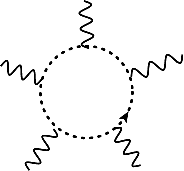
Refer to caption
Refer to caption
Figure 1: A 3-regular gluon cycle (left) and an oriented ghost cycle (right)

We have shown in [23] that we can impose the Slavnov–Taylor identities on the Hopf algebra HH, compatibly with the coproduct, equating all of the following formal elements:

Qk,k~:=(G/k,k~,/(G/2,0,/)k/2​(G/0,2~,/)k~/2)1/(k+k~−2),Q^{k,\widetilde{k}}:=\left(\frac{G^{k,\widetilde{k},/}_{/}}{(G^{2,0,/}_{/})^{k/2}(G^{0,\widetilde{2},/}_{/})^{\widetilde{k}/2}}\right)^{1/(k+\widetilde{k}-2)}, (17)

independent of the numbers kk and k~\widetilde{k} of external gluon and ghost edges, respectively. The thus-defined single formal series Q≡Qk,k~Q\equiv Q^{k,\widetilde{k}} will play the role of a ‘charge’ element in the Hopf algebra.

Proposition 5.1.

The coproduct on the Green’s functions read

Δ⁡(Gj3​j4;n~k,n)=∑jm=jm′+jm′′n=n′+n′′n~=n~′+n~′′(Gk,n′​Q2​n′′)j3′​j4′;n~′⊗Gj3′′​j4′′;n~′′k,n′′\Delta(G^{k,n}_{j_{3}j_{4};\widetilde{n}})=\sum_{\begin{smallmatrix}j_{m}=j^{\prime}_{m}+j^{\prime\prime}_{m}\\ n=n^{\prime}+n^{\prime\prime}\\ \widetilde{n}=\widetilde{n}^{\prime}+\widetilde{n}^{\prime\prime}\end{smallmatrix}}(G^{k,n^{\prime}}Q^{2n^{\prime\prime}})_{j_{3}^{\prime}j_{4}^{\prime};\widetilde{n}^{\prime}}\otimes G^{k,n^{\prime\prime}}_{j_{3}^{\prime\prime}j_{4}^{\prime\prime};\widetilde{n}^{\prime\prime}}

with Gj3​j4;n~k,nG^{k,n}_{j_{3}j_{4};\widetilde{n}} the above series of graphs of vertex multidegree (j3,j4)(j_{3},j_{4}), first Betti number nn and n~\widetilde{n} ghost cycles.

After taking the Slavnov–Taylor identities (17) into account, the coproduct reads on the above series of graphs

Δ⁡(Gk,n)=∑n=n′+n′′(Gk​Q2​n′′)n′⊗Gk,n′′.\Delta(G^{k,n})=\sum_{\begin{smallmatrix}n=n^{\prime}+n^{\prime\prime}\end{smallmatrix}}(G^{k}Q^{2n^{\prime\prime}})_{n^{\prime}}\otimes G^{k,n^{\prime\prime}}.
Remark 5.2.

Note that neither the lhs nor the rhs depend on k~\widetilde{k} in the above proposition, as Q≡Qk,k~Q\equiv Q^{k,\widetilde{k}}, ∀k,k~\forall k,\widetilde{k}.

Remark 5.3.

The inclusion of fermions is parallel to the study of ghost edges and loops, and a mere notational exercise.

Another way to describe the Green’s function GkG^{k} is in terms of so-called grafting operators, defined in terms of 1PI primitive graphs. We start by considering maps B+γ:H→AugB_{+}^{\gamma}:H\to\mathrm{Aug}, with Aug\mathrm{Aug} the augmentation ideal, which will soon lead us to non-trivial one co-cycles in the Hochschild cohomology of HH. They are defined as follows.

B+γ​(h)=∑Γ∈⟨Γ⟩bij​(γ,h,Γ)|h|∨​1maxf​(Γ)​1(γ|h)​Γ,B_{+}^{\gamma}(h)=\sum_{\Gamma\in\langle\Gamma\rangle}\frac{{\textbf{bij}(\gamma,h,\Gamma)}}{|h|_{\vee}}\frac{1}{\textrm{maxf}(\Gamma)}\frac{1}{(\gamma|h)}\Gamma,

where maxf(Γ)(\Gamma) is the number of maximal forests of Γ\Gamma, |h|∨|h|_{\vee} is the number of distinct graphs obtainable by permuting edges of hh, bij​(γ,h,Γ)\textbf{bij}(\gamma,h,\Gamma) is the number of bijections of external edges of hh with an insertion place in γ\gamma such that the result is Γ\Gamma, and finally (γ|h)(\gamma|h) is the number of insertion places for hh in γ\gamma [24]. ∑Γ∈<Γ>\sum_{\Gamma\in<\Gamma>} indicates a sum over the linear span ⟨Γ⟩\langle\Gamma\rangle of generators of HH.

The sum of the B+γB^{\gamma}_{+} over all primitive 1PI Feynman graphs at a given loop order and with given residue will be denoted by B+l;nB^{l;n}_{+}, as in [24]. More precisely,

B+k;n=∑γ​prim|γ|=nEE​(γ)=k1Sym⁡(γ)​B+γ.B^{k;n}_{+}=\sum_{\begin{smallmatrix}\gamma~\prim\\ |\gamma|=n\\ E_{E}(\gamma)=k\end{smallmatrix}}\frac{1}{\Sym(\gamma)}B^{\gamma}_{+}.

With this and the above Proposition, we can show [24, Theorem 5]:

Gk\displaystyle G^{k} =∑l=0∞B+k;n​(Gk​Q2​n);\displaystyle=\sum_{l=0}^{\infty}B_{+}^{k;n}(G^{k}Q^{2n}); (18)
Δ⁡(B+k;n​(Gk​Q2​n))\displaystyle\Delta(B_{+}^{k;n}(G^{k}Q^{2n})) =B+k;n​(Gk​Q2​n)⊗𝕀+(id⊗B+k;n)​Δ​(Gk​Q2​n).\displaystyle=B_{+}^{k;n}(G^{k}Q^{2n})\otimes\mathbb{I}+(\textup{id}\otimes B_{+}^{k;n})\Delta(G^{k}Q^{2n}). (19)

Equation (18) is known as the combinatorial Dyson–Schwinger equation, while (19) shows that B+k;nB_{+}^{k;n} is a Hochschild cocycle for the Hopf algebra HH.

5.3 The generator of ghost loops

We again consider the map δ+:H→H\delta_{+}:H\to H that replaces gluon loops in a Feynman graph by ghost loops.

Remark 5.4.

In accordance with our previous definition of δ+\delta_{+}, it becomes an algebra derivation δ+:H→H\delta_{+}:H\to H by the assignment

δ+​(Γ)=(l~+1)​∑g⊂ΓΓg↦g~.\delta_{+}(\Gamma)=(\widetilde{l}+1)\sum_{g\subset\Gamma}\Gamma_{g\mapsto\widetilde{g}}.

for a 1PI Feynman graph Γ\Gamma at ghost loop order l~\widetilde{l}. The sum is over all oriented 3-regular gluon cycles gg, and Γg↦g~\Gamma_{g\mapsto\widetilde{g}} denotes the graph Γ\Gamma with the 3-regular gluon cycle gg replaced by a ghost cycle g~\widetilde{g} (cf. Figure 1), of the same orientation.

The notation δ+\delta_{+} suggests that there is also a δ−\delta_{-}. In fact, such an operator can be defined and would replace a ghost loop by a gluon loop. We will not further study such an operator, since our interest lies in generating physical amplitudes from zero-ghost-loop amplitudes.

Example 5.5.

Consider the following one-loop gluon self-energy graph:

Γ=[Uncaptioned image].\Gamma=\parbox{28.45274pt}{\includegraphics[scale={.1}]{gluon1l2e.eps}}.

Its symmetry factor is Sym⁡(Γ)=2\Sym(\Gamma)=2 so that

δ+​([Uncaptioned image])=2​[Uncaptioned image].\delta_{+}\left(\parbox{28.45274pt}{\includegraphics[scale={.1}]{gluon1l2e.eps}}\right)=2\parbox{28.45274pt}{\includegraphics[scale={.1}]{ghost1l2e.eps}}.

A two loop example is given by the graph

Γ′=[Uncaptioned image]\Gamma^{\prime}=\parbox{42.67912pt}{\includegraphics[scale={.15}]{gluon2l2eA.eps}}

for which Sym⁡(Γ′)=2\Sym(\Gamma^{\prime})=2. Now,

δ+​([Uncaptioned image])=2​[Uncaptioned image]+2​[Uncaptioned image]+2​[Uncaptioned image].\delta_{+}\left(\parbox{42.67912pt}{\includegraphics[scale={.15}]{gluon2l2eA.eps}}\right)=2\parbox{56.9055pt}{\includegraphics[scale={.15}]{ghost2l2eA.eps}}+2\parbox{56.9055pt}{\includegraphics[scale={.15}]{ghost2l2eD.eps}}+2\parbox{56.9055pt}{\includegraphics[scale={.15}]{ghost2l2eDR.eps}}.

The first graph on the rhs obtains a factor of two because the two orientation of the ghost loop both reproduce this graph when the little gluon loop is replaced by a ghost loop.

The other two possible gluon cycles give the same graphs with again a coefficient of two for each of them, with the two orientations of the ghost cycle now resulting in those two remaining graphs on the rhs. In full accordance with Lemma 4.24, the ratio of the symmetry factor of a graph on the left by the symmetry factor of a graph on the right counts such multiplicities.

With that lemma we conclude:

Proposition 5.6.

When acting on series of graphs with no ghost cycles (n~=0\widetilde{n}=0):

eδ+∘B+k;n=∑γ​prim|γ|=n,n~​(γ)=0EE​(γ)=k1Sym⁡(γ)​B+eδ+​(γ)∘eδ+e^{\delta^{+}}\circ B_{+}^{k;n}=\sum_{\begin{smallmatrix}\gamma~\prim\\ |\gamma|=n,\widetilde{n}(\gamma)=0\\ E_{E}(\gamma)=k\end{smallmatrix}}\frac{1}{\Sym(\gamma)}B_{+}^{e^{\delta^{+}}(\gamma)}\circ e^{\delta_{+}}

where the sum is over graphs γ\gamma with no ghost cycles.

Remark 5.7.

There is a similar result for connected graphs on the exponentiation of χ+\chi_{+}. We give it here without proof. It follows directly though from extending the definition of graph Hopf algebras and their Hochschild cohomology from 1PI to connected graphs. When acting on series of graphs with no marked edges:

eχ+∘B+k;n=∑γ​prim|γ|=n,j⁡(γ)=0EE​(γ)=k1Sym⁡(γ)​B+eχ+​(γ)∘eχ+e^{\chi^{+}}\circ B_{+}^{k;n}=\sum_{\begin{smallmatrix}\gamma~\prim\\ |\gamma|=n,j(\gamma)=0\\ E_{E}(\gamma)=k\end{smallmatrix}}\frac{1}{\Sym(\gamma)}B_{+}^{e^{\chi^{+}}(\gamma)}\circ e^{\chi_{+}}

where the sum is over graphs γ\gamma with no marked edges and j⁡(γ)j(\gamma) is the number of 4-valent vertices.

Together, the two results on the interplay of Hochschild cohomology and exponentiation show that gauge invariant combinatorial Green functions are obtained from gauge invariant skeleton graphs into which gauge invariant subgraphs are inserted.

Example 5.8.

Let us consider the example of the gluon self-energy at two loops:

Gn=22\displaystyle G_{n=2}^{2} =+16​[Uncaptioned image]+12​[Uncaptioned image]+12​[Uncaptioned image]\displaystyle=+\frac{1}{6}\parbox{51.21495pt}{\includegraphics[scale={.15}]{tad2l2eB.eps}}+\frac{1}{2}\parbox{56.9055pt}{\includegraphics[scale={.15}]{gluon2l2eE.eps}}+\frac{1}{2}\parbox{56.9055pt}{\includegraphics[scale={.15}]{gluon2l2eF.eps}} (20)
+12​[Uncaptioned image]+[Uncaptioned image]+[Uncaptioned image]+[Uncaptioned image]\displaystyle\quad+\frac{1}{2}\parbox{56.9055pt}{\includegraphics[scale={.15}]{gluon2l2eA.eps}}+\parbox{56.9055pt}{\includegraphics[scale={.15}]{ghost2l2eA.eps}}+\parbox{56.9055pt}{\includegraphics[scale={.15}]{ghost2l2eD.eps}}+\parbox{56.9055pt}{\includegraphics[scale={.15}]{ghost2l2eDR.eps}}
+12​[Uncaptioned image]+[Uncaptioned image]+[Uncaptioned image]+[Uncaptioned image]\displaystyle\quad+\frac{1}{2}\parbox{56.9055pt}{\includegraphics[scale={.15}]{gluon2l2eB.eps}}+\parbox{56.9055pt}{\includegraphics[scale={.15}]{ghost2l2eB.eps}}+\parbox{56.9055pt}{\includegraphics[scale={.15}]{ghost2l2eC.eps}}+\parbox{56.9055pt}{\includegraphics[scale={.15}]{ghost2l2eE.eps}}

whose zero-ghost-loop part is

Gn=2,n~=02=16​[Uncaptioned image]+12​[Uncaptioned image]+12​[Uncaptioned image]\displaystyle G_{n=2,\widetilde{n}=0}^{2}=\frac{1}{6}\parbox{51.21495pt}{\includegraphics[scale={.15}]{tad2l2eB.eps}}+\frac{1}{2}\parbox{56.9055pt}{\includegraphics[scale={.15}]{gluon2l2eE.eps}}+\frac{1}{2}\parbox{56.9055pt}{\includegraphics[scale={.15}]{gluon2l2eF.eps}} (21)
+12​[Uncaptioned image]+12​[Uncaptioned image]\displaystyle\qquad+\frac{1}{2}\parbox{56.9055pt}{\includegraphics[scale={.15}]{gluon2l2eA.eps}}+\frac{1}{2}\parbox{56.9055pt}{\includegraphics[scale={.15}]{gluon2l2eB.eps}}

One readily checks that (1+δ+)​Gn=2,n~=02=Gn=22(1+\delta_{+})G_{n=2,\widetilde{n}=0}^{2}=G_{n=2}^{2}.

Theorem 5.9.

Let H~\widetilde{H} be the Hopf subalgebra of HH generated by Gk,nG^{k,n} for all n≥0n\geq 0 and k=2,3,4k=2,3,4. Then exp⁡δ+\exp{\delta_{+}} is an automorphisms of the graded Hopf algebra H~\widetilde{H}:

expδ+(x1x2)=expδ+(x1)expδ+(x2);Δ(expδ+(x))=(expδ+⊗expδ+)Δ(x).\exp{\delta_{+}}(x_{1}x_{2})=\exp{\delta_{+}}(x_{1})\exp{\delta_{+}}(x_{2});\qquad\Delta(\exp{\delta_{+}}(x))=(\exp{\delta_{+}}\otimes\exp{\delta_{+}})\Delta(x).

for x1,x2,x∈H~x_{1},x_{2},x\in\widetilde{H}.

Proof.

By definition, δ+\delta_{+} is an algebra derivation so that exp⁡δ+\exp\delta_{+} is an algebra automorphism. Note that at a given loop order ll, the exponential terminates at that power nn and is thus well-defined on the graded algebra underlying H~\widetilde{H}.

Let us then consider the compatibility of δ+\delta_{+} with the coproduct structure. Recall from [22] the formula

Δ⁡(Gk)=∑j3,j4,j~≥0Gk​(Q3)j3​(Q4)2​j4​(Q1,2~)n~⊗Gj3​j4​j~k.\Delta(G^{k})=\sum_{j_{3},j_{4},\widetilde{j}\geq 0}G^{k}(Q^{3})^{j_{3}}(Q^{4})^{2j_{4}}(Q^{1,\widetilde{2}})^{\widetilde{n}}\otimes G^{k}_{j_{3}j_{4}\widetilde{j}}.

which holds even without the Slavnov–Taylor identities. It continues to hold when restricting to graphs with zero ghost loops:

Δ⁡(Gn~=0k)=∑j3,j4Gn~=0k​(Qn~=03)j3​(Qn~=04)2​j4⊗Gj3,j4;n~=0r.\Delta(G^{k}_{\widetilde{n}=0})=\sum_{j_{3},j_{4}}G^{k}_{\widetilde{n}=0}(Q_{\widetilde{n}=0}^{3})^{j_{3}}(Q_{\widetilde{n}=0}^{4})^{2j_{4}}\otimes G^{r}_{j_{3},j_{4};\widetilde{n}=0}.

We now apply exp⁡δ+⊗exp⁡δ+\exp\delta_{+}\otimes\exp\delta_{+} to this equation to obtain after imposing the Slavnov–Taylor-identities Q3=Q4Q^{3}=Q^{4}:

(exp⁡δ+⊗exp⁡δ+)​Δ​(Gn~=0k)\displaystyle(\exp\delta_{+}\otimes\exp\delta_{+})\Delta(G^{k}_{\widetilde{n}=0}) =∑j3,j4Gk​(Q3)j3​(Q4)2​j4⊗exp⁡δ+​(Gj3​j4;n~=0k)\displaystyle=\sum_{j_{3},j_{4}}G^{k}(Q^{3})^{j_{3}}(Q^{4})^{2j_{4}}\otimes\exp\delta_{+}\left(G^{k}_{j_{3}j_{4};\widetilde{n}=0}\right)
=∑n≥0Gk​Q2​n⊗exp⁡δ+​(Gn,n~=0k)\displaystyle=\sum_{n\geq 0}G^{k}Q^{2n}\otimes\exp\delta_{+}\left(G^{k}_{n,\widetilde{n}=0}\right)

since in the absence of ghost vertices j3+2​j4=2​nj_{3}+2j_{4}=2n in terms of the first Betti number nn. Lemma(4.24) then yields exp⁡δ+​(Gn,n~=0k)=Gnk\exp\delta_{+}(G^{k}_{n,\widetilde{n}=0})=G^{k}_{n}, which completes the proof. ∎

This can be extended to the connected Green’s functions Xk,nX_{k,n}, where also a similar result can be shown for exp⁡χ+\exp\chi_{+}.

Example 5.10.

First, recall the Slavnov–Taylor identities G3​G2~=G1,2~​G2G^{3}G^{\widetilde{2}}=G^{1,\widetilde{2}}G^{2} which at one-loop order become:

[Uncaptioned image]+12​[Uncaptioned image]+[Uncaptioned image]+[Uncaptioned image]−[Uncaptioned image]−[Uncaptioned image]−[Uncaptioned image]+12​[Uncaptioned image]+[Uncaptioned image]=0.\parbox{56.9055pt}{\includegraphics[scale={.15}]{gluon1l3e.eps}}+\frac{1}{2}\parbox{56.9055pt}{\includegraphics[scale={.15}]{gluon1l3eA.eps}}+\parbox{42.67912pt}{\includegraphics[scale={.15}]{ghost1l3e.eps}}+\parbox{42.67912pt}{\includegraphics[scale={.15}]{ghost1l3eR.eps}}-\parbox{42.67912pt}{\includegraphics[scale={.15}]{gluon1l1e2ge.eps}}-\parbox{42.67912pt}{\includegraphics[scale={.15}]{ghost1l1e2ge.eps}}-\parbox{56.9055pt}{\includegraphics[scale={.15}]{gluon1l2ge.eps}}\\ +\frac{1}{2}\parbox{56.9055pt}{\includegraphics[scale={.15}]{gluon1l2e.eps}}+\parbox{56.9055pt}{\includegraphics[scale={.15}]{ghost1l2e.eps}}=0.

We compute Δ′​(Gn~=02,n=2)\Delta^{\prime}(G^{2,n=2}_{\widetilde{n}=0}) with Gn~=02,n=2G^{2,n=2}_{\widetilde{n}=0} given in Eq.(21). For the first graph on the last line, we have

Δ′​(12​[Uncaptioned image])=12​[Uncaptioned image]⊗[Uncaptioned image]\Delta^{\prime}\left(\frac{1}{2}\parbox{56.9055pt}{\includegraphics[scale={.15}]{gluon2l2eA.eps}}\right)=\frac{1}{2}\parbox{56.9055pt}{\includegraphics[scale={.15}]{gluon1l2e.eps}}\otimes\parbox{56.9055pt}{\includegraphics[scale={.15}]{gluon1l2e.eps}}

If we apply exp⁡δ+⊗exp⁡δ+\exp\delta_{+}\otimes\exp\delta_{+} to this expression, we obtain

12​([Uncaptioned image]+2​[Uncaptioned image])⊗([Uncaptioned image]+2​[Uncaptioned image])\frac{1}{2}\left(\parbox{56.9055pt}{\includegraphics[scale={.15}]{gluon1l2e.eps}}+2\parbox{56.9055pt}{\includegraphics[scale={.15}]{ghost1l2e.eps}}\right)\otimes\left(\parbox{56.9055pt}{\includegraphics[scale={.15}]{gluon1l2e.eps}}+2\parbox{56.9055pt}{\includegraphics[scale={.15}]{ghost1l2e.eps}}\right)

For the coproduct on the last graph in Eq.(21) we have

Δ′​(12​[Uncaptioned image])=[Uncaptioned image]⊗[Uncaptioned image]\Delta^{\prime}\left(\frac{1}{2}\parbox{56.9055pt}{\includegraphics[scale={.15}]{gluon2l2eB.eps}}\right)=\parbox{56.9055pt}{\includegraphics[scale={.15}]{gluon1l3e.eps}}\otimes\parbox{56.9055pt}{\includegraphics[scale={.15}]{gluon1l2e.eps}}

and applying exp⁡δ+⊗exp⁡δ+\exp\delta_{+}\otimes\exp\delta_{+} to this expression yields

([Uncaptioned image]+[Uncaptioned image]+[Uncaptioned image])⊗([Uncaptioned image]+2​[Uncaptioned image])\left(\parbox{56.9055pt}{\includegraphics[scale={.15}]{gluon1l3e.eps}}+\parbox{42.67912pt}{\includegraphics[scale={.15}]{ghost1l3e.eps}}+\parbox{42.67912pt}{\includegraphics[scale={.15}]{ghost1l3eR.eps}}\right)\otimes\left(\parbox{56.9055pt}{\includegraphics[scale={.15}]{gluon1l2e.eps}}+2\parbox{56.9055pt}{\includegraphics[scale={.15}]{ghost1l2e.eps}}\right)

On the other hand, Δ′​(exp⁡δ+​Gn~=02,n=2)=Δ′​(G2,n=2)\Delta^{\prime}(\exp\delta_{+}G^{2,n=2}_{\widetilde{n}=0})=\Delta^{\prime}(G^{2,n=2}) is computed from Eq.(20):

Δ′​(G2,n=2)=(12​[Uncaptioned image]+[Uncaptioned image])⊗[Uncaptioned image]+2[Uncaptioned image]⊗[Uncaptioned image]+([Uncaptioned image]+[Uncaptioned image]+[Uncaptioned image])⊗[Uncaptioned image]+(2[Uncaptioned image]+2[Uncaptioned image])⊗[Uncaptioned image]\Delta^{\prime}(G^{2,n=2})=\left(\frac{1}{2}\parbox{56.9055pt}{\includegraphics[scale={.15}]{gluon1l2e.eps}}+\parbox{56.9055pt}{\includegraphics[scale={.15}]{ghost1l2e.eps}}\right)\otimes\parbox{56.9055pt}{\includegraphics[scale={.15}]{gluon1l2e.eps}}\\ +2\parbox{42.67912pt}{\includegraphics[scale={.15}]{gluon1l2ge.eps}}\otimes\parbox{56.9055pt}{\includegraphics[scale={.15}]{ghost1l2e.eps}}\\ +\left(\parbox{56.9055pt}{\includegraphics[scale={.15}]{gluon1l3e.eps}}+\parbox{42.67912pt}{\includegraphics[scale={.15}]{ghost1l3e.eps}}+\parbox{42.67912pt}{\includegraphics[scale={.15}]{ghost1l3eR.eps}}\right)\otimes\parbox{56.9055pt}{\includegraphics[scale={.15}]{gluon1l2e.eps}}\\ +\left(2\parbox{34.1433pt}{\includegraphics[scale={.15}]{gluon1l1e2ge.eps}}+2\parbox{42.67912pt}{\includegraphics[scale={.15}]{ghost1l1e2ge.eps}}\right)\otimes\parbox{56.9055pt}{\includegraphics[scale={.15}]{ghost1l2e.eps}}

We conclude that

(exp⁡δ+⊗exp⁡δ+)​Δ′​(Gn~=02,n=2)−Δ′​(exp⁡δ+​(Gn~=02,n=2))=2​(12​[Uncaptioned image]+[Uncaptioned image]+[Uncaptioned image]+[Uncaptioned image]CLOSEOPEN−[Uncaptioned image]+[Uncaptioned image]−[Uncaptioned image]−[Uncaptioned image])⊗[Uncaptioned image](\exp\delta_{+}\otimes\exp\delta_{+})\Delta^{\prime}(G^{2,n=2}_{\widetilde{n}=0})-\Delta^{\prime}(\exp\delta_{+}(G^{2,n=2}_{\widetilde{n}=0}))=\\ 2\left(\frac{1}{2}\parbox{56.9055pt}{\includegraphics[scale={.15}]{gluon1l2e.eps}}+\parbox{56.9055pt}{\includegraphics[scale={.15}]{ghost1l2e.eps}}+\parbox{42.67912pt}{\includegraphics[scale={.15}]{ghost1l3e.eps}}+\parbox{42.67912pt}{\includegraphics[scale={.15}]{ghost1l3eR.eps}}\right.\\ \left.-\parbox{42.67912pt}{\includegraphics[scale={.15}]{gluon1l2ge.eps}}+\parbox{56.9055pt}{\includegraphics[scale={.15}]{gluon1l3e.eps}}-\parbox{42.67912pt}{\includegraphics[scale={.15}]{gluon1l1e2ge.eps}}-\parbox{42.67912pt}{\includegraphics[scale={.15}]{ghost1l1e2ge.eps}}\right)\otimes\parbox{56.9055pt}{\includegraphics[scale={.15}]{ghost1l2e.eps}}

which vanishes by the Slavnov–Taylor identities upon adding the contribution of 4-valent vertices.

6 The corolla polynomial and differentials

6.1 The Corolla Polynomial

Finally, we introduce the Corolla Polynomial ([10]). It is a polynomial based on half-edge variables av,ja_{v,j} assigned to any half-edge (v,j)(v,j) determined by a vertex vv and an edge jj. We need the following definitions:

  • •

    For a vertex v∈Vv\in V let n⁡(v)n(v) be the set of edges incident to vv (internal or external).

  • •

    For a vertex v∈Vv\in V let Dv=∑j∈n⁡(v)av,jD_{v}=\sum_{j\in n(v)}a_{v,j}.

  • •

    Let 𝒞\mathscr{C} be the set of all cycles of Γ\Gamma (cycles, not circuits). This is a finite set.

  • •

    For CC a cycle and vv a vertex in VV, since Γ\Gamma is 3-regular, there is a unique edge of Γ\Gamma incident to vv and not in CC, let vCv_{C} be this edge.

  • •

    For i≥0i\geq 0 let

    Ci=∑C1,C2,…​Ci∈𝒞Cj​pairwise disjoint((∏j=1i∏v∈Cjav,vC)​∏v∉C1∪C2∪⋯∪CiDv)C^{i}=\sum_{\begin{subarray}{c}C_{1},C_{2},\ldots C_{i}\in\mathscr{C}\\ C_{j}\text{pairwise disjoint}\end{subarray}}\left(\left(\prod_{j=1}^{i}\prod_{v\in C_{j}}a_{v,v_{C}}\right)\prod_{v\not\in C_{1}\cup C_{2}\cup\cdots\cup C_{i}}D_{v}\right)
  • •

    Let

    C=∑j≥0(−1)j​CjC=\sum_{j\geq 0}(-1)^{j}C^{j}

For any finite graph Γ\Gamma, this is a polynomial C=C⁡(Γ)C=C(\Gamma) —the corolla polynomial— because Ci=0C^{i}=0 for i>|𝒞|i>|\mathscr{C}|.

Theorem 6.1.

([10]) Let 𝒯Γ\mathscr{T}^{\Gamma} be the set of sets TT of half edges of Γ\Gamma with the property that

  • •

    every vertex of Γ\Gamma is incident to exactly one half edge of TT

  • •

    Γ∖T\Gamma\smallsetminus T has no cycles

Then

C⁡(Γ)=∑T∈𝒯Γ∏h∈TahC(\Gamma)=\sum_{T\in\mathscr{T}^{\Gamma}}\prod_{h\in T}a_{h}
Remark 6.2.

This shows that the corolla polynomial is strictly positive. As it applies in this form as a corolla differential to pure Yang–Mills theory, this results in a positivity statement on Yang–Mills theory which does not hold for gauge fields coupled to matter fields. Accordingly, the sign of the β\beta-function in gauge theory becomes dependent on the number of fermion families, and their representations.

Remark 6.3.

For a graph Γ\Gamma, let EE be a set of pairwise disjoint internal edges of Γ\Gamma. For i≥0i\geq 0 let

CEi​(Γ)=∑C1,C2,…​Ci∈𝒞Cj​ pairwise disjointCj∩E=∅((∏j=1i∏v∈Cjav,vC)​∏v∉C1∪C2∪⋯∪Ci∪EDv)C^{i}_{E}(\Gamma)=\sum_{\begin{subarray}{c}C_{1},C_{2},\ldots C_{i}\in\mathscr{C}\\ C_{j}\text{ pairwise disjoint}\\ C_{j}\cap E=\emptyset\end{subarray}}\left(\left(\prod_{j=1}^{i}\prod_{v\in C_{j}}a_{v,v_{C}}\right)\prod_{v\not\in C_{1}\cup C_{2}\cup\cdots\cup C_{i}\cup E}D_{v}\right)

where the sum forbids cycles from sharing either vertices or edges with EE.

Let

CE​(Γ)=∑j≥0(−1)j​CEj​(Γ).C_{E}(\Gamma)=\sum_{j\geq 0}(-1)^{j}C^{j}_{E}(\Gamma).

Then,

CE​(Γ)=C⁡(Γ−E)C_{E}(\Gamma)=C(\Gamma-E)

where Γ−E\Gamma-E is the graph with the edges and vertices involved in EE removed. Removing a vertex removes all its incident half-edges so that 2​|E|2|E| new external edges are generated. Note that C∅​(Γ)=C⁡(Γ)C_{\emptyset}(\Gamma)=C(\Gamma).

Define

Cfr​(Γ):=∑E(CE​(Γ)​∏e∈EWe),C^{\mathrm{fr}}(\Gamma):=\sum_{E}\left(C_{E}(\Gamma)\prod_{e\in E}W_{e}\right),

where WeW_{e} is defined in (7).

Corollary 6.4.
Cfr​(Γ)=∑E(∑T∈𝒯E(∏h∈Tah)​∏e∈EWe).C^{\mathrm{fr}}(\Gamma)=\sum_{E}\left(\sum_{T\in\mathscr{T}^{E}}(\prod_{h\in T}a_{h})\prod_{e\in E}W_{e}\right).
Proof.

Immediate. ∎

Remark 6.5.

Consider a 3-regular graph Γ\Gamma which has jj, j≥2j\geq 2, 3-valent vertices, and let 𝒫\mathscr{P} be a set of mm paths, 2​m≤j2m\leq j, on internal edges and 3-valent vertices in Γ\Gamma which each connect two external 3-valent vertices (a 3-valent vertex vv is external if n⁡(v)n(v) contains an external edge) with pi∩pj=∅p_{i}\cap p_{j}=\emptyset, ∀pi,pj∈𝒫\forall p_{i},p_{j}\in\mathscr{P}.

Consider for chosen set EE and 𝒫\mathscr{P} as above, with E∩𝒫=∅E\cap\mathscr{P}=\emptyset, for i≥0i\geq 0,

CE,𝒫i​(Γ)\displaystyle C^{i}_{E,\mathscr{P}}(\Gamma) =\displaystyle= ∑C1,C2,…​Ci∈𝒞Cj​ pairwise disjointCj∩E=∅Cj∩𝒫=∅((∏j=1i∏v∈Cjav,vC)∏v∉C1∪C2∪⋯∪Ci∪E∪𝒫Dv)×\displaystyle\sum_{\begin{subarray}{c}C_{1},C_{2},\ldots C_{i}\in\mathscr{C}\\ C_{j}\text{ pairwise disjoint}\\ C_{j}\cap E=\emptyset\\ C_{j}\cap\mathscr{P}=\emptyset\end{subarray}}\left(\left(\prod_{j=1}^{i}\prod_{v\in C_{j}}a_{v,v_{C}}\right)\prod_{v\not\in C_{1}\cup C_{2}\cup\cdots\cup C_{i}\cup E\cup\mathscr{P}}D_{v}\right)\times
×(∏p∈𝒫∏v∈pav,vp),\displaystyle\times\left(\prod_{p\in\mathscr{P}}\prod_{v\in p}a_{v,v_{p}}\right),

where the sum forbids cycles from sharing either vertices or edges with EE, and vpv_{p} is the unique half-edge at vv not in pp.

Let

CE,𝒫​(Γ)=∑j≥0(−1)j​CE,𝒫j​(Γ).C_{E,\mathscr{P}}(\Gamma)=\sum_{j\geq 0}(-1)^{j}C^{j}_{E,\mathscr{P}}(\Gamma).

Finally, we set

C𝒫fr​(Γ):=∑E(CE,𝒫​(Γ)​∏e∈EWe).C^{\mathrm{fr}}_{\mathscr{P}}(\Gamma):=\sum_{E}\left(C_{E,\mathscr{P}}(\Gamma)\prod_{e\in E}W_{e}\right). (22)

6.2 Corolla differentials

Our main use of the corolla polynomial is to construct differential operators with it. These operators differentiate with respect to momenta ξe\xi_{e} assigned to edges ee of a graph, and act on the second Kirchhoff polynomial written for generic edge momenta ξe\xi_{e}, that is on |N|Pf|N|_{\mathrm{Pf}}.

Only at the end of the computation will we employ the map

Q:ξe→ξe+q⁡(e).Q:\xi_{e}\to\xi_{e}+q(e).

We then set ξe=0\xi_{e}=0 after we have applied the corolla differentials so that we obtain the standard second Symanzik polynomial for specific external momenta as prescribed by gauge theory amplitudes.

For a half edge h≡(w,f)∈HΓh\equiv(w,f)\in H^{\Gamma}, we let e⁡(h)=fe(h)=f and v⁡(h)=wv(h)=w. We remind the reader that h+h_{+} and h−h_{-} are the successor and the precursor of hh in the oriented corolla at v⁡(h)v(h), and that we assign to a graph Γ\Gamma:

  1. i.

    to each (possibly external) edge ee, a variable AeA_{e} and a 4-vector ξe\xi_{e};

  2. ii.

    to each half edge hh, a Lorentz index μ⁡(h)\mu(h);

  3. iii.

    a factor colour⁡(Γ)\mathrm{colour}(\Gamma).

6.3 The differential D0D^{0}

The corolla polynomial is an alternating sum over terms CiC^{i}, where ii counts the number of loops. Similarly, the corolla differentials are a sum of terms DiD^{i}. We start with D0D^{0}.

Let Γ∈𝒢n,l\Gamma\in\mathscr{G}^{n,l}:

U0(Γ)=∫Ed​k¯L(2​π)d​lCΓ0(D¯)e−∑e∈Γ[1]Aeξe′2,U^{0}(\Gamma)=\int_{E}\frac{\mathrm{d}\underline{k}_{L}}{(2\pi)^{dl}}C_{\Gamma}^{0}(\underline{D})e^{-\sum_{e\in\Gamma^{[1]}}A_{e}\xi_{e}^{\prime 2}},

where

CΓ0​(D¯)=∏v∈Γ[0]Dv,Dv=Dv​1+Dv​2+Dv​3C_{\Gamma}^{0}(\underline{D})=\prod_{v\in\Gamma^{[0]}}D_{v},\qquad D_{v}=D_{v1}+D_{v2}+D_{v3}

(the edges incident on vv are labelled 1,2,31,2,3),

Dv​1=−12​gμ2​μ3​(εv​2​1A2​∂∂ξ2​μ1−εv​3​1A3​∂∂ξ3​μ1).D_{v1}=-\tfrac{1}{2}g^{\mu_{2}\mu_{3}}\Big(\varepsilon_{v2}\frac{1}{A_{2}}\frac{\partial}{\partial\xi_{2\mu_{1}}}-\varepsilon_{v3}\frac{1}{A_{3}}\frac{\partial}{\partial\xi_{3\mu_{1}}}\Big).

Using that all corollas are oriented, we can write this as

Dg​(h):=−12​gμh+​μh−​(εh+​1Ae⁡(h+)​∂∂ξ​(h+)μh−εh−​1Ae⁡(h−)​∂∂ξ​(h−)μh),D_{g}(h):=-\tfrac{1}{2}g^{\mu_{h_{+}}\mu_{h_{-}}}\Big(\varepsilon_{h_{+}}\frac{1}{A_{e(h_{+})}}\frac{\partial}{\partial\xi(h_{+})_{\mu_{h}}}-\varepsilon_{h_{-}}\frac{1}{A_{e(h_{-})}}\frac{\partial}{\partial\xi(h_{-})_{\mu_{h}}}\Big),

for any half-edge hh. The operator DvD_{v} is such that if it acts on e−∑e∈Γ[1]Aeξe′2e^{-\sum_{e\in\Gamma^{[1]}}A_{e}\xi_{e}^{\prime 2}}, it gives the 3-vertex Feynman rule of Eq.(10):

Dve−∑e∈Γ[1]Aeξe′2=V(3)ve−∑e∈Γ[1]Aeξe′2.D_{v}e^{-\sum_{e\in\Gamma^{[1]}}A_{e}\xi_{e}^{\prime 2}}=V^{(3)}_{v}e^{-\sum_{e\in\Gamma^{[1]}}A_{e}\xi_{e}^{\prime 2}}.

In order to calculate CΓ0​(D¯)≡CΓ0​(h→Dg​(h))C_{\Gamma}^{0}(\underline{D})\equiv C_{\Gamma}^{0}(h\to D_{g}(h)), we also need to know the Leibniz terms Dv​Vw(3)D_{v}V^{(3)}_{w}, where v,w∈Γ[0]v,w\in\Gamma^{[0]}.

  • •

    If vv and ww do not share an edge, Dv​Vw(3)=0D_{v}V^{(3)}_{w}=0.

  • •

    Suppose they share exactly one edge; we give it label 55. Let 11 and 22 be the other edges at vv and 33 and 44 the other ones at ww:

    ††feynman-diagram: (Feynman diagram, (x3).\parbox[c][35.0pt]{35.0pt}{\centering\begin{fmfgraph*}{3}0,30) \end{fmfgraph*}\@add@centering}.

    Then:

    Dv​Vw(3)=1A5​(gμ4​μ2​gμ3​μ1−gμ2​μ3​gμ4​μ1)≡WeAe,D_{v}V^{(3)}_{w}=\frac{1}{A_{5}}(g^{\mu_{4}\mu_{2}}g^{\mu_{3}\mu_{1}}-g^{\mu_{2}\mu_{3}}g^{\mu_{4}\mu_{1}})\equiv\frac{W_{e}}{A_{e}},

    where WeW_{e} is the Feynman rule for a marked edge (equation (7)). Note that thus

    Dv​Vw(3)=Dw​Vv(3).D_{v}V^{(3)}_{w}=D_{w}V^{(3)}_{v}.
  • •

    Suppose that vv and ww share two edges, 33 and 44. Let 11 be the other edge at vv and 22 the other one at ww:

    ††feynman-diagram: (Feynman diagram, (x3).\parbox[c][35.0pt]{35.0pt}{\centering\begin{fmfgraph*}{3}0,15) \end{fmfgraph*}\@add@centering}.

    Then:

    Dv​Vw(3)=(1A3​(gμ4​μ4​gμ2​μ1−gμ2​μ4​gμ4​μ1)+1A4​(gμ3​μ3​gμ2​μ1−gμ3​μ2​gμ3​μ1))=W3A3+W4A4.\begin{split}D_{v}V^{(3)}_{w}&=\Big(\frac{1}{A_{3}}(g^{\mu_{4}\mu_{4}}g^{\mu_{2}\mu_{1}}-g^{\mu_{2}\mu_{4}}g^{\mu_{4}\mu_{1}})+\frac{1}{A_{4}}(g^{\mu_{3}\mu_{3}}g^{\mu_{2}\mu_{1}}-g^{\mu_{3}\mu_{2}}g^{\mu_{3}\mu_{1}})\Big)\\ &=\frac{W_{3}}{A_{3}}+\frac{W_{4}}{A_{4}}.\end{split}

    where we have used equation (7). Note that also in this case

    Dv​Vw(3)=Dw​Vv(3).D_{v}V^{(3)}_{w}=D_{w}V^{(3)}_{v}.

    Contracting the indices further gives self-loops which can be omitted:

    Dv​Vw(3)=3​C2​δa1​a2​gμ1​μ2​(1A3+1A4).D_{v}V^{(3)}_{w}=3C_{2}\delta^{a_{1}a_{2}}g^{\mu_{1}\mu_{2}}\Big(\frac{1}{A_{3}}+\frac{1}{A_{4}}\Big).

6.4 Regular terms and residues

We can now compute immediately the application of D0D^{0} to the scalar integrand IΓI_{\Gamma}, that is, U0​(Γ):=D0​IΓU^{0}(\Gamma):=D^{0}I_{\Gamma}.

U0​(Γ)=∫d​k¯L(2​π)d​l(∏v∈Γ[0]Dv)e−∑e∈Γ[1]Aeξe′2=∫d​k¯L(2​π)d​l[(∏v∈Γ[0]V(3)v)+∑w,w′∈Γ[0]w and w′ share an edgew<w′(DwV(3)w′)(∏v∈Γ[0]v≠w,w′V(3)v)+∑w,w′,x,x′∈Γ[0]w and w′ and x and x′ share an edgew<w′<x<x′(DwV(3)w′)(DxV(3)x′)(∏v∈Γ[0]v≠w,w′,x,x′V(3)v)+⋯]e−∑e∈Γ[1]Aeξe′2.\begin{split}U^{0}(\Gamma)&=\int\frac{\mathrm{d}\underline{k}_{L}}{(2\pi)^{dl}}\bigg(\prod_{v\in\Gamma^{[0]}}D_{v}\bigg)e^{-\sum_{e\in\Gamma^{[1]}}A_{e}\xi_{e}^{\prime 2}}\\ &=\int\frac{\mathrm{d}\underline{k}_{L}}{(2\pi)^{dl}}\bigg[\bigg(\prod_{v\in\Gamma^{[0]}}V^{(3)}_{v}\bigg)\\ &\qquad+\sum_{\begin{subarray}{c}w,w^{\prime}\in\Gamma^{[0]}\\ \text{$w$ and $w^{\prime}$ share an edge}\\ w<w^{\prime}\end{subarray}}(D_{w}V^{(3)}_{w^{\prime}})\bigg(\prod_{\begin{subarray}{c}v\in\Gamma^{[0]}\\ v\neq w,w^{\prime}\end{subarray}}V^{(3)}_{v}\bigg)\\ &\qquad+\sum_{\begin{subarray}{c}w,w^{\prime},x,x^{\prime}\in\Gamma^{[0]}\\ \text{$w$ and $w^{\prime}$ and $x$ and $x^{\prime}$ share an edge}\\ w<w^{\prime}<x<x^{\prime}\end{subarray}}(D_{w}V^{(3)}_{w^{\prime}})(D_{x}V^{(3)}_{x^{\prime}})\bigg(\prod_{\begin{subarray}{c}v\in\Gamma^{[0]}\\ v\neq w,w^{\prime},x,x^{\prime}\end{subarray}}V^{(3)}_{v}\bigg)\\ &\qquad+\cdots\bigg]e^{-\sum_{e\in\Gamma^{[1]}}A_{e}\xi_{e}^{\prime 2}}.\end{split}

With the result of the previous subsection we get (recall that we exclude graphs with self-loops):

U0​(Γ)=∫d​k¯L(2​π)d​l[(∏v∈Γ[0]V(3)v)+∑e∈Γint[1]WeAe(∏v∈Γ[0]v​ not adj. to ​eV(3)v)+∑{e1,e2}⊂Γint[1]e1 and e2 do not share a vertexWe1​We2Ae1​Ae2(∏v∈Γ[0]v​ not adj. to ​e1,e2V(3)v)+⋯]e−∑e′∈Γ[1]Ae′ξe′′2.=∑k≥0∑{e1,…,ek}⊂Γint[1]e1,…,ek do not share a vertexWe1⋯WekAe1⋯Aek​∫d​k¯L(2​π)d​l×(∏v∈Γ[0]v​ not adj. to ​e1,…,ekV(3)v)e−∑e∈Γ[1]Aeξe′2.\begin{split}U^{0}(\Gamma)&=\int\frac{\mathrm{d}\underline{k}_{L}}{(2\pi)^{dl}}\bigg[\bigg(\prod_{v\in\Gamma^{[0]}}V^{(3)}_{v}\bigg)+\sum_{e\in\Gamma^{[1]}_{\rm int}}\frac{W_{e}}{A_{e}}\bigg(\prod_{\begin{subarray}{c}v\in\Gamma^{[0]}\\ v\text{ not adj.\ to }e\end{subarray}}V^{(3)}_{v}\bigg)\\ &\qquad+\sum_{\begin{subarray}{c}\{e_{1},e_{2}\}\subset\Gamma^{[1]}_{\rm int}\\ \text{$e_{1}$ and $e_{2}$ do not share a vertex}\end{subarray}}\frac{W_{e_{1}}W_{e_{2}}}{A_{e_{1}}A_{e_{2}}}\bigg(\prod_{\begin{subarray}{c}v\in\Gamma^{[0]}\\ v\text{ not adj.\ to }e_{1},e_{2}\end{subarray}}V^{(3)}_{v}\bigg)\\ &\qquad+\cdots\bigg]e^{-\sum_{e^{\prime}\in\Gamma^{[1]}}A_{e^{\prime}}\xi_{e^{\prime}}^{\prime 2}}.\\ &=\sum_{k\geq 0}\sum_{\begin{subarray}{c}\{e_{1},\ldots,e_{k}\}\subset\Gamma^{[1]}_{\rm int}\\ \text{$e_{1},\ldots,e_{k}$ do not share a vertex}\end{subarray}}\frac{W_{e_{1}}\cdots W_{e_{k}}}{A_{e_{1}}\cdots A_{e_{k}}}\int\frac{\mathrm{d}\underline{k}_{L}}{(2\pi)^{dl}}\\ &\qquad\times\bigg(\prod_{\begin{subarray}{c}v\in\Gamma^{[0]}\\ v\text{ not adj.\ to }e_{1},\ldots,e_{k}\end{subarray}}V^{(3)}_{v}\bigg)e^{-\sum_{e\in\Gamma^{[1]}}A_{e}\xi_{e}^{\prime 2}}.\\ \end{split}

The first term we recognise as the Feynman-Schwinger integrand of Γ\Gamma. The other terms we can write as the integrands of marked versions of Γ\Gamma (equation (9)). More precisely,

U0(Γ)=∑k≥0∑{e1,…,ek}⊂Γint[1]1Ae1⋯Aek∫d​k¯L(2​π)d​lℐ(χ+e1⋯χ+ekΓ)e−Ae1​ξe1′2−⋯−Aek​ξek′2,U^{0}(\Gamma)=\sum_{k\geq 0}\sum_{\{e_{1},\ldots,e_{k}\}\subset\Gamma^{[1]}_{\rm int}}\frac{1}{A_{e_{1}}\cdots A_{e_{k}}}\int\frac{\mathrm{d}\underline{k}_{L}}{(2\pi)^{dl}}\mathscr{I}(\chi_{+}^{e_{1}}\cdots\chi_{+}^{e_{k}}\Gamma)e^{-A_{e_{1}}\xi_{e_{1}}^{\prime 2}-\cdots-A_{e_{k}}\xi_{e_{k}}^{\prime 2}},

where ℐ⁡(Γ)\mathscr{I}(\Gamma) is given in equation (11). Recall that in the exponent in the integrand only the unmarked edges are included. That is why the factor e−Ae1​ξe1′2−⋯−Aek​ξek′2e^{-A_{e_{1}}\xi_{e_{1}}^{\prime 2}-\cdots-A_{e_{k}}\xi_{e_{k}}^{\prime 2}} appears. This factor does not change the residue along ∏e∈Γint[1]Ae=0\prod_{e\in\Gamma^{[1]}_{\rm int}}A_{e}=0.

Each subset of edges here is accompanied by a corresponding set of poles. By construction, the residues along these poles correspond to integrands where the edges shrink to form 4-valent vertices with the correct Feynman rules.

Using the χ+e\chi_{+}^{e}-operator, we can write the integral U~0​(Γ)\widetilde{U}^{0}(\Gamma) as:

U~0​(Γ)=∑k≥0∑{e1,…,ek}⊂Γint[1]∫dA¯Γ[1]∖{e1,…,ek}I(χ+e1⋯χ+ekΓ).\begin{split}\widetilde{U}^{0}(\Gamma)&=\sum_{k\geq 0}\sum_{\{e_{1},\ldots,e_{k}\}\subset\Gamma^{[1]}_{\rm int}}\int\mathrm{d}\underline{A}_{\Gamma^{[1]}\smallsetminus\{e_{1},\ldots,e_{k}\}}I(\chi_{+}^{e_{1}}\cdots\chi_{+}^{e_{k}}\Gamma).\end{split}

In terms of Feynman amplitudes, this is

U~0(Γ)=∑k≥0∑{e1,…,ek}⊂Γint[1]Φ(χ+e1⋯χ+ekΓ)=Φ(eχ+Γ).\widetilde{U}^{0}(\Gamma)=\sum_{k\geq 0}\sum_{\{e_{1},\ldots,e_{k}\}\subset\Gamma^{[1]}_{\rm int}}\Phi(\chi_{+}^{e_{1}}\cdots\chi_{+}^{e_{k}}\Gamma)=\Phi(e^{\chi_{+}}\Gamma). (23)

Instead of applying U~0\widetilde{U}^{0} to a single graph, we can do this to the combinatorial Green’s function Xn,lX^{n,l}. This gives us the Green’s function for all graphs in Yang–Mills theory without the ghosts, but including the 4-valent vertices:

Proposition 6.6.

Collecting residues as above produces the evaluation by the Feynman rules of all 3- and 4-valent graphs in gauge theory without internal ghost or fermion edges:

U~0​(Xn,l)=Φ⁡(eχ+​Xn,l)=Φ⁡(X/[Uncaptioned image]n,l).\widetilde{U}^{0}(X^{n,l})=\Phi(e^{\chi_{+}}X^{n,l})=\Phi(X^{n,l}_{/{\includegraphics[]{fourvertex-index.eps}}}).
Proof.

The above equation (23) is used, together with Lemma 4.10.iii. ∎

6.5 Exponentiating residues

Let us discuss the pairing between the integrand with poles along the boundaries of the simplex, with boundaries given by σΓ:∏i=1|ΓI[1]|Ai=0\sigma_{\Gamma}:\prod_{i=1}^{|\Gamma_{I}^{[1]}|}A_{i}=0, and the Feynman integrand U0​(Γ)U^{0}(\Gamma) in more detail.

The amplitude U~0​(Γ)\widetilde{U}^{0}(\Gamma) can be obtained from U0​(Γ)U^{0}(\Gamma) by taking residues along hypersurfaces ∏e∈EAe=0\prod_{e\in E}A_{e}=0 and regular parts and integrating:

U~0​(Γ)=∑k≥0∑{e1,…,ek}⊂Γint[1]∫d​A¯Γ[1]∖{e1,…,ek}​RegA1,…,Ae1^,…,Aek^,…=0​ResAe1,…,Aek=0U0​(Γ).\begin{split}\widetilde{U}^{0}(\Gamma)&=\sum_{k\geq 0}\sum_{\{e_{1},\ldots,e_{k}\}\subset\Gamma^{[1]}_{\rm int}}\int\mathrm{d}\underline{A}_{\Gamma^{[1]}\smallsetminus\{e_{1},\ldots,e_{k}\}}\Reg_{A_{1},\ldots,\widehat{A_{e_{1}}},\ldots,\widehat{A_{e_{k}}},\ldots=0}\Res_{A_{e_{1}},\ldots,A_{e_{k}}=0}U^{0}(\Gamma).\end{split}

For a function f=f⁡({Ae})f=f(\{A_{e}\}) of graph polynomial variables Ae,e∈γI[1]A_{e},e\in\gamma^{[1]}_{I} with at most simple poles at the origin localized in disjoint sets of edges EE, we can write

f=∑EfE,f=\sum_{E}f^{E},

where the sum is over all such sets and fEf_{E} is the part of ff which is regular upon setting variables Ae,e∈(ΓI[1]−E)A_{e},e\in(\Gamma^{[1]}_{I}-E) to zero.

For any set EE of mutually disjoint internal edges of Γ\Gamma, consider ∏e∈E∮γef,\prod_{e\in E}\oint_{\gamma_{e}}f, and let fEf^{E} be its regular part. For any finite graph Γ\Gamma, let ℰγ\mathscr{E}^{\gamma} be the set of all sets of mutually disjoint edges (∅\emptyset included).

Consider the differential form

JΓf:=(fE​⋀e∈(ΓI[1]−E)d​Ae)E∈ℰΓ.J_{\Gamma}^{f}:=\Big(f^{E}\bigwedge_{e\in(\Gamma^{[1]}_{I}-E)}dA_{e}\Big)_{E\in\mathscr{E}^{\Gamma}}.

Let MΓEM_{\Gamma}^{E} be the hypercube

MΓE:=ℝ+|ΓI[1]|−|E|,M_{\Gamma}^{E}:=\mathbb{R}_{+}^{|\Gamma^{[1]}_{I}|-|E|},

and the corresponding vector

HΓ​(MΓE)E∈ℰΓ.H_{\Gamma}(M_{\Gamma}^{E})_{E\in\mathscr{E}^{\Gamma}}.

Then, there is a natural pairing

∫HΓ⋅JΓf:=∑E∈ℰΓ∫MΓE(fE​⋀e∈(ΓI[1]−E)d​Ae).\int H_{\Gamma}\cdot J_{\Gamma}^{f}:=\sum_{E\in\mathscr{E}^{\Gamma}}\int_{M_{\Gamma}^{E}}\Big(f^{E}\bigwedge_{e\in(\Gamma^{[1]}_{I}-E)}dA_{e}\Big).

6.6 Graph homology and the residue map

Note that in parametric integration we integrate against the simplex σ≡σΓ\sigma\equiv\sigma_{\Gamma} with boundary ∏e∈Γ[1]Ae=0\prod_{e\in\Gamma^{[1]}}A_{e}=0. We have co-dimension kk-hypersurfaces given by

Ai1=⋯=Aik=0.A_{i_{1}}=\cdots=A_{i_{k}}=0.

The Feynman integrand we have constructed above comes from regular parts, and residues along these hypersurfaces. It can be described by the following commutative diagram.

𝒢j[Uncaptioned image],/[Uncaptioned image]∋Γ→χ+χ+(Γ)∈𝒢(j+1)[Uncaptioned image],/[Uncaptioned image]↓Φ↓ΦΦ⁡(Γ)→∑eReseΦ​(χ+​(Γ))\begin{CD}\mathscr{G}_{j{\includegraphics[]{fourvertex-index.eps}},/{\includegraphics[]{ghostloop-index.eps}}}\ni\Gamma @>{\chi_{+}}>{}>\chi_{+}(\Gamma)\in\mathscr{G}_{(j+1){\includegraphics[]{fourvertex-index.eps}},/{\includegraphics[]{ghostloop-index.eps}}}\\ @V{}V{\Phi}V@V{}V{\Phi}V\\ \Phi(\Gamma)@>{\sum_{e}\mathrm{Res}_{e}}>{}>\Phi(\chi_{+}(\Gamma))\end{CD}

The underlying geometry will be interpreted elsewhere.

6.7 Covariant gauges

For an edge ee, let

Gμ​νρ​(e):=gμ​νξe′2−2​ρ​ξe′μ​ξe′νξe′4G_{\mu\nu}^{\rho}(e):=\frac{g_{\mu\nu}}{{{\xi_{e}^{\prime}}}^{2}}-2\rho\frac{{\xi_{e}^{\prime}}_{\mu}{\xi_{e}^{\prime}}_{\nu}}{{{\xi_{e}^{\prime}}}^{4}}

the corresponding gluon propagator in a covariant gauge (ρ=1/2\rho=1/2 being the transversal Landau gauge, ρ=0\rho=0 the Feynman gauge). One computes

Gμ​νρ​(e)=∫0∞−12​A​ρ​∂∂ξe​μ′​∂∂ξe​ν′​e−ρ​A​ξe′2​𝑑A=:∫0∞gμ​νρ​(e)​𝑑A.G_{\mu\nu}^{\rho}(e)=\int_{0}^{\infty}\frac{-1}{2A\rho}\frac{\partial}{\partial\xi^{\prime}_{e\mu}}\frac{\partial}{\partial\xi^{\prime}_{e\nu}}e^{-\rho A{{\xi_{e}^{\prime}}^{2}}}d\!A=:\int_{0}^{\infty}g_{\mu\nu}^{\rho}(e)d\!A.

We set

GΓρ:=∏e∈ΓI[1]Gμ(s⁡(e),e)​μ(t⁡(e),e)ρ​(e),G^{\rho}_{\Gamma}:=\prod_{e\in\Gamma^{[1]}_{I}}G^{\rho}_{\mu_{(s(e),e)}\mu_{(t(e),e)}}(e),

for half-edges (s⁡(e),e)(s(e),e) and (t⁡(e),e)(t(e),e), and gΓρg^{\rho}_{\Gamma} accordingly.

We let IΓ​(ρ)I_{\Gamma}(\rho) be the corresponding scalar integrand obtained by substituting Ae→ρ​AeA_{e}\to\rho A_{e} for each internal edge ee.

GΓρG^{\rho}_{\Gamma} acts as a differential operator so that

GΓρ​IΓ​(ρ)=FG​(ρ)​IΓ​(ρ),G^{\rho}_{\Gamma}I_{\Gamma}(\rho)=F_{G}(\rho)I_{\Gamma}(\rho),

with FG​(ρ)F_{G}(\rho) a polynomial in ρ\rho, edge variables AeA_{e} and 4-momenta ξe\xi_{e}.

Similarly, the corolla differential DΓD_{\Gamma} acts as a differential operator so that

DΓ​IΓ​(1)=FD​IΓ​(1),D_{\Gamma}I_{\Gamma}(1)=F_{D}I_{\Gamma}(1),

with FDF_{D} a polynomial in the 4-momenta ξe\xi_{e} and a rational function in the edge variables AeA_{e}.

To compute in an arbitrary covariant gauge, we then work with

FG​(ρ)​FD​IΓ​(1).F_{G}(\rho)F_{D}I_{\Gamma}(1).

6.8 Yang–Mills theory

Consider a cycle CC through 3-valent vertices in a graph Γ\Gamma, and consider

∏v∈CDg​(vC).\prod_{v\in C}D_{g}(v_{C}).\

This is a differential operator with coefficients which are monomials in variables 1/Ae1/A_{e}, where e∈Ce\in C.

Let DCD_{C} be the part in this differential operator which is linear in all variables 1/Ae1/A_{e}, for e∈Ce\in C. Let ϕC\phi_{C} be the Feynman rule for a ghost loop on CC, summed over both orientations.

Lemma 6.7.
ϕC:=DCe−∑e∈CAeξe′2.\phi_{C}:=D_{C}e^{-\sum_{e\in C}A_{e}{\xi_{e}^{\prime}}^{2}}.
Proof.

This follows directly from the Feynman rules for ghost propagators and ghost-gluon vertices. Linearization eliminates all poles with residues corresponding to 4-valent 2-ghost-2-gluon vertices. ∎

Now consider the corolla polynomial C⁡(Γ)C(\Gamma) and replace each half-edge variable hh by the differential Dg​(h)D_{g}(h). This defines a differential operator

d​(Γ)YM:=C⁡(Γ)​(h→Dg​(h)),d(\Gamma)^{\mathrm{YM}}:=C(\Gamma)(h\to D_{g}(h)),

We consider d​(Γ)YM​(IΓ)d(\Gamma)^{\mathrm{YM}}(I_{\Gamma}) where

IΓ:=e−|NΓ|PfψΓψΓ2,I_{\Gamma}:=\frac{e^{-\frac{|N_{\Gamma}|_{\mathrm{Pf}}}{\psi_{\Gamma}}}}{\psi_{\Gamma}^{2}},

is the scalar integrand for a graph Γ\Gamma.

Proposition 6.8.

All poles in d​(Γ)YM​IΓd(\Gamma)^{\mathrm{YM}}I_{\Gamma} are located along co-dimension |E||E| hypersurfaces Ae=0,e∈EA_{e}=0,\;e\in E for subsets EE of mutually disjoint edges are simple poles.

Proof.

Corollary 3.6 ensures that poles are at most of first order and appear only when two derivatives act on the same edge. By the definition of the corolla polynomial this can only appear in mutually disjoint ordered pairs of corollas. All poles coming from divergent subgraphs are located along subsets of connected edges, as divergent subgraphs have more than a single edge. ∎

By our previous results on the Leibniz terms we can summarize now for the parametric integrand:

Corollary 6.9.

The residues of these poles correspond to graphs where each corresponding pair of corollas PeP_{e} is replaced by a 4-valent vertex.

Proof.

Setting an edge variable to zero shrinks that edge in the two Symanzik polynomials by the standard contraction-deletion identities [2, 3, 25]. ∎

The Leibniz terms serve the useful purpose to shrink an edge between two 3-gluon vertices. They provide a residue which corresponds to the integrand where the corresponding edge is a marked edge in our conventions. it is hence part of the integrand for a graph with a corresponding 4-valent vertex. As we have checked before, when summing over all connected 3-regular graphs, we correctly reproduce the Feynman integrand for all gluon self-interactions.

We stress that in doing so we want to shrink edges only between pairs of corollas which both are corollas for 3-gluon vertices, and will not mark edges between other type of vertices. This leads us to

Definition 6.10.

We let D​(Γ)YM​IΓD(\Gamma)^{\mathrm{YM}}I_{\Gamma} be the part d​(Γ)YM​IΓd(\Gamma)^{\mathrm{YM}}I_{\Gamma} which is linear in all variables 1/Ae1/A_{e}.

This eliminates all poles in D​(Γ)YM​IΓD(\Gamma)^{\mathrm{YM}}I_{\Gamma} of the form 1/Ae1/A_{e}. We can regain then the contribution of 4-valent 4-gluon vertices by using Theorem 6.1 together with Remark 6.3:

Lemma 6.11.

Let

UΓ=gΓρ​Cfr​(Γ)​(ah→Dg​(h))​IΓ.U_{\Gamma}=g^{\rho}_{\Gamma}C^{\mathrm{fr}}(\Gamma)(a_{h}\to D_{g}(h))I_{\Gamma}.

Then U¯Γ\overline{U}_{\Gamma} (cf. Eq.(5)) generates the integrand for the complete contribution of Γ\Gamma to the full Yang–Mills theory amplitude. U¯ΓR\overline{U}_{\Gamma}^{R} generates the corresponding integrand for the renormalized contribution.

Proof.

Immediate application of Lemma 6.7 and Theorem 1.3. ∎

This also proves Theorem 1.5 in the context of Yang–Mills theory.

Remark 6.12.

If we were to work with non-linear gauges, we could avoid this linearization and use the Leibniz terms for the graphs with 2-gluon 2-ghost and 4-ghost vertices. Also, note that U¯ΓR=U¯ΓR​(ρ)\overline{U}_{\Gamma}^{R}=\overline{U}_{\Gamma}^{R}(\rho) depends on the gauge parameter.

6.9 Amplitudes with open ghost or fermion lines

For kk open ghost lines we have a straightforward generalization of these differentials by using C𝒫fr​(G)C^{\mathrm{fr}}_{\mathscr{P}}(G), see Eq.(22), where each half edge hh is again replaced by Dg​(h)D_{g}(h) and linearization is understood as before. For fermion lines, see below.

6.10 Gauge Theory

If we include matter fields, we need to add a second differential in particular for fermion fields:

Df​(h)\displaystyle D_{f}(h) :⁣=\displaystyle:= (1A⁡(e⁡(h+))​∂∂ξ​(e⁡(h+))μ⁡(h+)​γμ⁡(h+)​γμ⁡(h)CLOSE\displaystyle\left(\frac{1}{A(e(h_{+}))}\frac{\partial}{\partial\xi(e(h_{+}))_{\mu(h_{+})}}\gamma_{\mu(h_{+})}\gamma_{\mu(h)}\right.
OPEN−1A⁡(e⁡(h−))​∂∂ξ​(e⁡(h−))μ⁡(h−)​γμ⁡(h)​γμ⁡(h−)).\displaystyle-\left.\frac{1}{A(e(h_{-}))}\frac{\partial}{\partial\xi(e(h_{-}))_{\mu(h_{-})}}\gamma_{\mu(h)}\gamma_{\mu(h_{-})}\right).

Now we must carefully distinguish between fermion and ghost cycles.

For a collection of cycles C1,⋯,CjC_{1},\cdots,C_{j} contributing to CjC^{j}, consider partitions of this set into two subsets If,IgI_{f},I_{g} containing |If|+|Ig|=j|I_{f}|+|I_{g}|=j cycles. Replace av,vC→bv,vCa_{v,v_{C}}\to b_{v,v_{C}} for each C∈IfC\in I_{f}. This defines CIg,If​(Γ)​(ah,bh)C^{I_{g},I_{f}}(\Gamma)(a_{h},b_{h}). Upon summing over all possible partitions Ig,IlI_{g},I_{l} of the cycles for each jj, this gives a further corolla polynomial for which we write in slight abuse of notation C⁡(Γ)​(ah,bh)C(\Gamma)(a_{h},b_{h}). Assign a differential operator as follows:

UΓ=gΓρ​∑j≥0∑|Ig|+|If|=jCIg,If​(Γ)​(Dg​(h),Df​(h))​colourIg,If​(Γ),U_{\Gamma}=g^{\rho}_{\Gamma}\sum_{j\geq 0}\sum_{|I_{g}|+|I_{f}|=j}C^{I_{g},I_{f}}(\Gamma)(D_{g}(h),D_{f}(h))\mathrm{colour}^{I_{g},I_{f}}(\Gamma),

where in CIg,IfC^{I_{g},I_{f}}, for Ig∪If≠∅I_{g}\cup I_{f}\not=\emptyset, we keep only terms which are linear in variables 1/Ae1/A_{e} for edges e∈C1∪⋯∪Cje\in C_{1}\cup\cdots\cup C_{j}. We can now proceed with U¯γ\overline{U}_{\gamma} as before.

Note that the restriction to Il=∅I_{l}=\emptyset gives back the corresponding operator for Yang–Mills theory. From here on, Theorem 1.5 follows for gauge theory as before for Yang–Mills theory.

Remark 6.13.

Note that all this can be turned into a projective integrand, illuminating the slots in the period matrix which are filled in a gauge theory as compared to a scalar field theory. In particular, one hopes that the geometry of Eq.(6.6) is helpful to explain appearances and disappearances of periods in gauge theory.

Remark 6.14.

Putting fermions into the same colour rep as gauge bosons allows for immediate cancellations between DgD_{g} and DfD_{f}. This can be illuminating in studying the simplifications for supersymmetric gauge theories.

6.11 Examples: QED and Yang–Mills theory

In the following two examples, we compute the one-loop vacuum polarization in quantum electrodynamics, and then the one-loop gluon vacuum polarization in Yang–Mills theory. Both examples can be obtained from corolla differentials acting on the simplest possible 3-regular graph:

Γ:=††feynman-diagram: (Feynman diagram, (x3).\Gamma:=\parbox{45.0pt}{\centering\scriptsize\begin{fmfgraph*}{3}5,17.5) \end{fmfgraph*}\@add@centering}.

We label its two internal edges 1,21,2, and the external edges 3,43,4. We also label the two vertices a,ba,b. Edge 3 is oriented from vertex aa to vertex bb, and edge 4 vice versa, say.

We have six half-edges: h1:=(a,3),h2:=(a,2),h3:=(a,1)h_{1}:=(a,3),h_{2}:=(a,2),h_{3}:=(a,1) and h4:=(b,1),h5:=(b,2),h6:=(b,4)h_{4}:=(b,1),h_{5}:=(b,2),h_{6}:=(b,4), with corresponding half-edge variables aa​3,aa​2a_{a3},a_{a2} etc.

We have four 4-vectors ξ1,ξ2,ξ3,ξ4\xi_{1},\xi_{2},\xi_{3},\xi_{4}, with ξe∈𝕄4\xi_{e}\in\mathbb{M}^{4}, Minkowski space, with scalar product ξe2≡ξe⋅ξe=ξe02−ξe12−ξe22−ξe32\xi_{e}^{2}\equiv\xi_{e}\cdot\xi_{e}={\xi_{e}}_{0}^{2}-{\xi_{e}}_{1}^{2}-{\xi_{e}}_{2}^{2}-{\xi_{e}}_{3}^{2}.

Example 6.15.

In order to compute the one-loop vacuum polarisation in massless QED,

Π1=††feynman-diagram: (Feynman diagram, (x2)\Pi_{1}=\parbox{25.0pt}{\begin{fmfgraph*}{2}5,12.5) \end{fmfgraph*}}

we proceed as follows. We have for the corolla polynomial

C1​(Γ)=aa​3​ab​4.C_{1}(\Gamma)=a_{a3}a_{b4}.

The scalar integrand is

I⁡(Γ)=12​ξ32​ξ42​e−(ξ1−ξ2)2​A1​A2+(A3​ξ32+A4​ξ42)​(A1+A2)A1+A2(A1+A2)2​d​A1​d​A2​d​A3​d​A4.I(\Gamma)=\frac{1}{2}{\xi_{3}}^{2}{\xi_{4}}^{2}\frac{e^{-\frac{({\xi_{1}}-{\xi_{2}})^{2}A_{1}A_{2}+(A_{3}{\xi_{3}}^{2}+A_{4}{\xi_{4}}^{2})(A_{1}+A_{2})}{A_{1}+A_{2}}}}{(A_{1}+A_{2})^{2}}dA_{1}dA_{2}dA_{3}dA_{4}.

We can directly integrate A3,A4A_{3},A_{4} eliminating any appearance of ξ32,ξ42{\xi_{3}}^{2},{\xi_{4}}^{2} as in this example no derivatives with respect to external edges appear in the corolla differential.

Indeed, replacing the two half-edge variables in C1​(Γ)C_{1}(\Gamma) by the fermion differential and using the linearized corolla differential (we symmetrize below in μ⁡(3),μ⁡(4)\mu(3),\mu(4) when allowed)

14​A1​A2​(∂∂ξ3μ⁡(3)​∂∂ξ4μ⁡(4)+∂∂ξ4μ⁡(4)​∂∂ξ3μ⁡(3))=12​A1​A2​∂∂ξ3μ⁡(3)​∂∂ξ4μ⁡(4)\frac{1}{4A_{1}A_{2}}\left(\frac{\partial}{\partial{\xi_{3}}_{\mu(3)}}\frac{\partial}{\partial{\xi_{4}}_{\mu(4)}}+\frac{\partial}{\partial{\xi_{4}}_{\mu(4)}}\frac{\partial}{\partial{\xi_{3}}_{\mu(3)}}\right)=\frac{1}{2A_{1}A_{2}}\frac{\partial}{\partial{\xi_{3}}_{\mu(3)}}\frac{\partial}{\partial{\xi_{4}}_{\mu(4)}}

delivers π1\pi_{1}, the integrand for Π1\Pi_{1}:

π1\displaystyle\pi_{1} :⁣=\displaystyle:= −14​Tr⁡(γμ⁡(3)​γμ⁡(2)​γμ⁡(4)​γμ⁡(1))​∂A1​∂ξ1μ⁡(1)​∂A2​∂ξ2μ⁡(2)​I​(Γ)\displaystyle-\frac{1}{4}\Tr(\gamma_{\mu(3)}\gamma_{\mu(2)}\gamma_{\mu(4)}\gamma_{\mu(1)})\frac{\partial}{A_{1}\partial{\xi_{1}}_{\mu(1)}}\frac{\partial}{A_{2}\partial{\xi_{2}}_{\mu(2)}}I(\Gamma)
=\displaystyle= −Tr(γμ⁡(3)γμ⁡(2)γμ⁡(4)γμ⁡(1))(ξ1−ξ2)μ⁡(1)(ξ2−ξ1)μ⁡(2)A1A2×\displaystyle-\Tr(\gamma_{\mu(3)}\gamma_{\mu(2)}\gamma_{\mu(4)}\gamma_{\mu(1)})({\xi_{1}}-{\xi_{2}})_{\mu(1)}({\xi_{2}}-{\xi_{1}})_{\mu(2)}A_{1}A_{2}\times
×e−(ξ1−ξ2)2​A1​A2A1+A2(A1+A2)4​d​A1​d​A2​(AγF1=A1​A2(A1+A2)4,|AγF1|γ=0)\displaystyle\times\frac{e^{-\frac{({\xi_{1}}-{\xi_{2}})^{2}A_{1}A_{2}}{A_{1}+A_{2}}}}{(A_{1}+A_{2})^{4}}dA_{1}dA_{2}\,\left(A_{\gamma}^{F_{1}}=\frac{A_{1}A_{2}}{(A_{1}+A_{2})^{4}},\,|A_{\gamma}^{F_{1}}|_{\gamma}=0\right)
+Tr(γμ⁡(3)γμ⁡(2)γμ⁡(4)γμ⁡(1))12gμ⁡(1)​μ​(2)×\displaystyle+\Tr(\gamma_{\mu(3)}\gamma_{\mu(2)}\gamma_{\mu(4)}\gamma_{\mu(1)})\frac{1}{2}g_{\mu(1)\mu(2)}\times
×e−(ξ1−ξ2)2​A1​A2A1+A2(A1+A2)3​d​A1​d​A2​(AγF2=1(A1+A2)3,|AγF2|γ=2).\displaystyle\times\frac{e^{-\frac{({\xi_{1}}-{\xi_{2}})^{2}A_{1}A_{2}}{A_{1}+A_{2}}}}{(A_{1}+A_{2})^{3}}dA_{1}dA_{2}\,\left(A_{\gamma}^{F_{2}}=\frac{1}{(A_{1}+A_{2})^{3}},\,|A_{\gamma}^{F_{2}}|_{\gamma}=2\right).

Partially integrating the metric tensor term (equivalently, multiplying AγF2A_{\gamma}^{F_{2}} by A1​A2(A1+A2)​A4\frac{A_{1}A_{2}}{(A_{1}+A_{2})A_{4}} before integrating A4A_{4}, see Eq.(5)) gives

π1\displaystyle\pi_{1} =\displaystyle= Tr(γμ⁡(3)γμ⁡(2)γμ⁡(4)γμ⁡(1))(ξ1−ξ2)μ⁡(1)(ξ2−ξ1)μ⁡(2)A1A2×\displaystyle\Tr(\gamma_{\mu(3)}\gamma_{\mu(2)}\gamma_{\mu(4)}\gamma_{\mu(1)})({\xi_{1}}-{\xi_{2}})_{\mu(1)}({\xi_{2}}-{\xi_{1}})_{\mu(2)}A_{1}A_{2}\times
×e−(ξ1−ξ2)2​A1​A2A1+A2(A1+A2)4​d​A1​d​A2\displaystyle\times\frac{e^{-\frac{({\xi_{1}}-{\xi_{2}})^{2}A_{1}A_{2}}{A_{1}+A_{2}}}}{(A_{1}+A_{2})^{4}}dA_{1}dA_{2}
+Tr(γμ⁡(3)γμ⁡(2)γμ⁡(4)γμ⁡(1))12gμ⁡(1)​μ​(2)(ξ1−ξ2)2A1A2×\displaystyle+\Tr(\gamma_{\mu(3)}\gamma_{\mu(2)}\gamma_{\mu(4)}\gamma_{\mu(1)})\frac{1}{2}g_{\mu(1)\mu(2)}({\xi_{1}}-{\xi_{2}})^{2}A_{1}A_{2}\times
×e−(ξ1−ξ2)2​A1​A2A1+A2(A1+A2)4​d​A1​d​A2.\displaystyle\times\frac{e^{-\frac{({\xi_{1}}-{\xi_{2}})^{2}A_{1}A_{2}}{A_{1}+A_{2}}}}{(A_{1}+A_{2})^{4}}dA_{1}dA_{2}.

Evaluating the trace, contracting indices and integrating delivers (QQ replaces ξ1−ξ2{\xi_{1}}-{\xi_{2}} by qq, subtraction at q2=μ2q^{2}=\mu^{2} understood, i.e. Q0Q_{0} replaces ξ1−ξ2{\xi_{1}}-{\xi_{2}} by μ\mu)

Π1=8(q2gμ⁡(3)​μ​(4)−qμ⁡(3)qμ⁡(4))∫A1​A2​e−q2​A1​A2A1+A2(A1+A2)4−⋯|q2=μ2dA1dA2\Pi_{1}=8(q^{2}g_{\mu(3)\mu(4)}-q_{\mu(3)}q_{\mu(4)})\int\frac{A_{1}A_{2}e^{-\frac{q^{2}A_{1}A_{2}}{A_{1}+A_{2}}}}{(A_{1}+A_{2})^{4}}-\cdots_{|q^{2}=\mu^{2}}dA_{1}dA_{2}

which can be written projectively

Π1=8​(q2​gμ⁡(3)​μ​(4)−qμ⁡(3)​qμ⁡(4))​ln⁡q2μ2​∫ℙ1​(ℝ+)A1​A2(A1+A2)4​(A1​d​A2−A2​d​A1)\Pi_{1}=8(q^{2}g_{\mu(3)\mu(4)}-q_{\mu(3)}q_{\mu(4)})\ln\frac{q^{2}}{\mu^{2}}\int_{\mathbb{P}^{1}(\mathbb{R}_{+})}\frac{A_{1}A_{2}}{(A_{1}+A_{2})^{4}}(A_{1}dA_{2}-A_{2}dA_{1})

and which correctly evaluates to the expected transversal result

Π1=43​(q2​gμ⁡(3)​μ​(4)−qμ⁡(3)​qμ⁡(4))​ln⁡q2μ2.\Pi_{1}=\frac{4}{3}(q^{2}g_{\mu(3)\mu(4)}-q_{\mu(3)}q_{\mu(4)})\ln\frac{q^{2}}{\mu^{2}}.

Next, we turn to Yang–Mills theory.

Example 6.16.

We have

|N††feynman-diagram: (Feynman diagram, (x1)|Pfψ††feynman-diagram: (Feynman diagram, (x1)\displaystyle\frac{|N_{{\parbox{10.0pt}{\begin{fmfgraph}{1}0,10/2) \end{fmfgraph}}}}|_{\mathrm{Pf}}}{\psi_{{\parbox{10.0pt}{\begin{fmfgraph}{1}0,10/2) \end{fmfgraph}}}}} =−ξ32​A3−ξ42​A4−(ξ1−ξ2)2​A1​A2A1+A2\displaystyle=-\xi_{3}^{2}A_{3}-\xi_{4}^{2}A_{4}-\frac{(\xi_{1}-\xi_{2})^{2}A_{1}A_{2}}{A_{1}+A_{2}}
while the corolla polynomials read
C††feynman-diagram: (Feynman diagram, (x1)0​(a¯)\displaystyle C_{{\parbox{10.0pt}{\begin{fmfgraph}{1}0,10/2) \end{fmfgraph}}}}^{0}(\underline{a}) =(aa3+aa1+aa2)​(ab4+ab1+ab2)\displaystyle=(a_{\rm a3}+a_{\rm a1}+a_{\rm a2})(a_{\rm b4}+a_{\rm b1}+a_{\rm b2})
C††feynman-diagram: (Feynman diagram, (x1)1​(a¯)\displaystyle C_{{\parbox{10.0pt}{\begin{fmfgraph}{1}0,10/2) \end{fmfgraph}}}}^{1}(\underline{a}) =aa3​ab4\displaystyle=a_{\rm a3}a_{\rm b4}

The corresponding differentials then become

C††feynman-diagram: (Feynman diagram, (x1)0​(D¯)=(Da3+Da1+Da2)​(Db4+Db2+Db1)=(−12)2​(gμ1​μ2​(−1A1​∂∂ξ1​μ3−1A2​∂∂ξ2​μ3)CLOSE+gμ2​μ3​(1A2​∂∂ξ2​μ1−1A3​∂∂ξ3​μ1)OPEN+gμ3​μ1​(1A3​∂∂ξ3​μ2+1A1​∂∂ξ1​μ2))×(gμ2​μ1​(−1A2​∂∂ξ2​μ4−1A1​∂∂ξ1​μ4)CLOSE+gμ1​μ4​(1A1​∂∂ξ1​μ2−1A4​∂∂ξ4​μ2)OPEN+gμ4​μ2​(1A4​∂∂ξ4​μ1+1A2​∂∂ξ2​μ1))C††feynman-diagram: (Feynman diagram, (x1)1​(D¯)=Da3​Db4=4​(−12)2​(−1A1​∂∂ξ1​μ3−1A2​∂∂ξ2​μ3)×(−1A2​∂∂ξ2​μ4−1A1​∂∂ξ1​μ4)\begin{split}C_{{\parbox{10.0pt}{\begin{fmfgraph}{1}0,10/2) \end{fmfgraph}}}}^{0}(\underline{D})&=(D_{\rm a3}+D_{\rm a1}+D_{\rm a2})(D_{\rm b4}+D_{\rm b2}+D_{\rm b1})\\ &=\big(-\tfrac{1}{2})^{2}\bigg(g^{\mu_{1}\mu_{2}}\Big(-\frac{1}{A_{1}}\frac{\partial}{\partial\xi_{1\mu_{3}}}-\frac{1}{A_{2}}\frac{\partial}{\partial\xi_{2\mu_{3}}}\Big)\\ &\qquad\quad+g^{\mu_{2}\mu_{3}}\Big(\frac{1}{A_{2}}\frac{\partial}{\partial\xi_{2\mu_{1}}}-\frac{1}{A_{3}}\frac{\partial}{\partial\xi_{3\mu_{1}}}\Big)\\ &\qquad\quad+g^{\mu_{3}\mu_{1}}\Big(\frac{1}{A_{3}}\frac{\partial}{\partial\xi_{3\mu_{2}}}+\frac{1}{A_{1}}\frac{\partial}{\partial\xi_{1\mu_{2}}}\Big)\bigg)\\ &\qquad\times\bigg(g^{\mu_{2}\mu_{1}}\Big(-\frac{1}{A_{2}}\frac{\partial}{\partial\xi_{2\mu_{4}}}-\frac{1}{A_{1}}\frac{\partial}{\partial\xi_{1\mu_{4}}}\Big)\\ &\qquad\quad+g^{\mu_{1}\mu_{4}}\Big(\frac{1}{A_{1}}\frac{\partial}{\partial\xi_{1\mu_{2}}}-\frac{1}{A_{4}}\frac{\partial}{\partial\xi_{4\mu_{2}}}\Big)\\ &\qquad\quad+g^{\mu_{4}\mu_{2}}\Big(\frac{1}{A_{4}}\frac{\partial}{\partial\xi_{4\mu_{1}}}+\frac{1}{A_{2}}\frac{\partial}{\partial\xi_{2\mu_{1}}}\Big)\bigg)\\ C_{{\parbox{10.0pt}{\begin{fmfgraph}{1}0,10/2) \end{fmfgraph}}}}^{1}(\underline{D})&=D_{\rm a3}D_{\rm b4}\\ &=4\big(-\tfrac{1}{2}\big)^{2}\Big(-\frac{1}{A_{1}}\frac{\partial}{\partial\xi_{1\mu_{3}}}-\frac{1}{A_{2}}\frac{\partial}{\partial\xi_{2\mu_{3}}}\Big)\\ &\qquad\times\Big(-\frac{1}{A_{2}}\frac{\partial}{\partial\xi_{2\mu_{4}}}-\frac{1}{A_{1}}\frac{\partial}{\partial\xi_{1\mu_{4}}}\Big)\end{split}

for which the linear part, without the factor 44 (the space-time dimension), is

C~††feynman-diagram: (Feynman diagram, (x1)1​(D¯)=(−12)2​1A1​A2​(∂2∂ξ1​μ3​∂ξ2​μ4+∂2∂ξ2​μ4​∂ξ1​μ3)\begin{split}\widetilde{C}_{{\parbox{10.0pt}{\begin{fmfgraph}{1}0,10/2) \end{fmfgraph}}}}^{1}(\underline{D})&=\big(-\tfrac{1}{2}\big)^{2}\frac{1}{A_{1}A_{2}}\Big(\frac{\partial^{2}}{\partial\xi_{1\mu_{3}}\partial\xi_{2\mu_{4}}}+\frac{\partial^{2}}{\partial\xi_{2\mu_{4}}\partial\xi_{1\mu_{3}}}\Big)\end{split}

We compute

U††feynman-diagram: (Feynman diagram, (x1)0\displaystyle U_{{\parbox{10.0pt}{\begin{fmfgraph}{1}0,10/2) \end{fmfgraph}}}}^{0} =C††feynman-diagram: (Feynman diagram, (x1)0​(D¯)​eϕ¯††feynman-diagram: (Feynman diagram, (x1)/ψ††feynman-diagram: (Feynman diagram, (x1)ψ††feynman-diagram: (Feynman diagram, (x1)2\displaystyle=C_{{\parbox{10.0pt}{\begin{fmfgraph}{1}0,10/2) \end{fmfgraph}}}}^{0}(\underline{D})\frac{e^{\overline{\phi}_{{\parbox{10.0pt}{\begin{fmfgraph}{1}0,10/2) \end{fmfgraph}}}}/\psi_{{\parbox{10.0pt}{\begin{fmfgraph}{1}0,10/2) \end{fmfgraph}}}}}}{\psi_{{\parbox{10.0pt}{\begin{fmfgraph}{1}0,10/2) \end{fmfgraph}}}}^{2}}
=1(A1+A2)4​((A1−A2)​gμ1​μ2​qμ3−(2​A1+A2)​gμ2​μ3​qμ1CLOSE\displaystyle=\frac{1}{(A_{1}+A_{2})^{4}}\Big((A_{1}-A_{2})g^{\mu_{1}\mu_{2}}q^{\mu_{3}}-(2A_{1}+A_{2})g^{\mu_{2}\mu_{3}}q^{\mu_{1}}
OPEN+(A1+2​A2)​gμ3​μ1​qμ2)​((A1−A2)​gμ2​μ1​qμ4CLOSE\displaystyle\qquad\qquad+(A_{1}+2A_{2})g^{\mu_{3}\mu_{1}}q^{\mu_{2}}\Big)\Big((A_{1}-A_{2})g^{\mu_{2}\mu_{1}}q^{\mu_{4}}
OPEN+(A1+2​A2)​gμ1​μ4​qμ2−(2​A1+A2)​gμ4​μ2​qμ1)\displaystyle\qquad\qquad+(A_{1}+2A_{2})g^{\mu_{1}\mu_{4}}q^{\mu_{2}}-(2A_{1}+A_{2})g^{\mu_{4}\mu_{2}}q^{\mu_{1}}\Big)
×e−q2​(A1​A2A1+A2+A3+A4)\displaystyle\qquad\quad\times e^{-q^{2}\big(\frac{A_{1}A_{2}}{A_{1}+A_{2}}+A_{3}+A_{4}\big)}
+3(A1+A2)3​(1−A1A2−A2A1⏞→0,as​residues​are​scale−independent​self−loops)​gμ1​μ2​e−q2​(A1​A2A1+A2+A3+A4)\displaystyle\qquad+\frac{3}{(A_{1}+A_{2})^{3}}\Big(1-\overbrace{\frac{A_{1}}{A_{2}}-\frac{A_{2}}{A_{1}}}^{\to 0,\,\mathrm{as\,residues\,are\,scale-independent\,self-loops}}\Big)g^{\mu_{1}\mu_{2}}e^{-q^{2}\big(\frac{A_{1}A_{2}}{A_{1}+A_{2}}+A_{3}+A_{4}\big)}
and so
U~††feynman-diagram: (Feynman diagram, (x1)0\displaystyle\widetilde{U}_{{\parbox{10.0pt}{\begin{fmfgraph}{1}0,10/2) \end{fmfgraph}}}}^{0} =(1(A1+A2)4​(−(2​A12+2​A22+14​A1​A2)​qμ3​qμ4CLOSECLOSE\displaystyle=\left(\frac{1}{(A_{1}+A_{2})^{4}}\big(-(2A_{1}^{2}+2A_{2}^{2}+14A_{1}A_{2})q^{\mu_{3}}q^{\mu_{4}}\right.
OPENOPEN+(5​A12+5​A22+8​A1​A2)​q2​gμ3​μ4))hence​|AγF1|γ=0​e−q2​A1​A2A1+A2​d​A1​d​A2\displaystyle\qquad\quad\left.+(5A_{1}^{2}+5A_{2}^{2}+8A_{1}A_{2})q^{2}g^{\mu_{3}\mu_{4}}\big)\right)_{\mathrm{hence}\,|A_{\gamma}^{F_{1}}|_{\gamma}=0}e^{-q^{2}\frac{A_{1}A_{2}}{A_{1}+A_{2}}}\mathrm{d}A_{1}\mathrm{d}A_{2}
+(3(A1+A2)3​gμ3​μ4)hence​|AγF2|γ=2​e−q2​A1​A2A1+A2​d​A1​d​A2\displaystyle\qquad+\left(\frac{3}{(A_{1}+A_{2})^{3}}g^{\mu_{3}\mu_{4}}\right)_{\mathrm{hence}\,|A_{\gamma}^{F_{2}}|_{\gamma}=2}e^{-q^{2}\frac{A_{1}A_{2}}{A_{1}+A_{2}}}\mathrm{d}A_{1}\mathrm{d}A_{2}

Similarly,

U~††feynman-diagram: (Feynman diagram, (x1)1=(2​A1​A2(A1+A2)4​qμ3​qμ4−1(A1+A2)3​gμ3​μ4)​e−q2​A1​A2A1+A2​d​A1​d​A2\begin{split}\widetilde{U}_{{\parbox{10.0pt}{\begin{fmfgraph}{1}0,10/2) \end{fmfgraph}}}}^{1}&=\Big(\frac{2A_{1}A_{2}}{(A_{1}+A_{2})^{4}}q^{\mu_{3}}q^{\mu_{4}}-\frac{1}{(A_{1}+A_{2})^{3}}g^{\mu_{3}\mu_{4}}\Big)e^{-q^{2}\frac{A_{1}A_{2}}{A_{1}+A_{2}}}\mathrm{d}A_{1}\mathrm{d}A_{2}\end{split}

We thus obtain for the corresponding integrals:

∫U~††feynman-diagram: (Feynman diagram, (x1)0​R=(113​qμ3​qμ4−256​q2​gμ3​μ4)​ln⁡(q2μ2),\begin{split}\int\widetilde{U}_{{\parbox{10.0pt}{\begin{fmfgraph}{1}0,10/2) \end{fmfgraph}}}}^{0\rm R}&=\big(\tfrac{11}{3}q^{\mu_{3}}q^{\mu_{4}}-\tfrac{25}{6}q^{2}g^{\mu_{3}\mu_{4}})\ln\Big(\frac{q^{2}}{\mu^{2}}\Big),\end{split}

which corresponds to the gauge boson loop:

††feynman-diagram: (Feynman diagram, (x2),\parbox{25.0pt}{\begin{fmfgraph*}{2}5,12.5) \end{fmfgraph*}},

and

∫U~††feynman-diagram: (Feynman diagram, (x1)1​R=−(13​qμ3​qμ4+16​q2​gμ3​μ4)​ln⁡(q2μ2),\int\widetilde{U}_{{\parbox{10.0pt}{\begin{fmfgraph}{1}0,10/2) \end{fmfgraph}}}}^{1\rm R}=-\big(\tfrac{1}{3}q^{\mu_{3}}q^{\mu_{4}}+\tfrac{1}{6}q^{2}g^{\mu_{3}\mu_{4}})\ln\Big(\frac{q^{2}}{\mu^{2}}\Big), (24)

which corresponds to the ghost loop:

††feynman-diagram: (Feynman diagram, (x2).\parbox{25.0pt}{\begin{fmfgraph*}{2}5,12.5) \end{fmfgraph*}}.

They combine to a transversal result:

∫U~††feynman-diagram: (Feynman diagram, (x1)R=∫U~††feynman-diagram: (Feynman diagram, (x1)0​R−∫U~††feynman-diagram: (Feynman diagram, (x1)1​R=4​(qμ3​qμ4−q2​gμ3​μ4)​ln⁡(q2μ2).\begin{split}\int\widetilde{U}_{{\parbox{10.0pt}{\begin{fmfgraph}{1}0,10/2) \end{fmfgraph}}}}^{\rm R}&=\int\widetilde{U}_{{\parbox{10.0pt}{\begin{fmfgraph}{1}0,10/2) \end{fmfgraph}}}}^{0\rm R}-\int\widetilde{U}_{{\parbox{10.0pt}{\begin{fmfgraph}{1}0,10/2) \end{fmfgraph}}}}^{1\rm R}\\ &=4(q^{\mu_{3}}q^{\mu_{4}}-q^{2}g^{\mu_{3}\mu_{4}})\ln\Big(\frac{q^{2}}{\mu^{2}}\Big).\end{split}

Multiplying with colour⁡(γ)sym⁡(γ)=12​fh1​h2​h3​fh2​h3​h6\frac{\mathrm{colour}(\gamma)}{\mathrm{sym}(\gamma)}=\frac{1}{2}f^{h_{1}h_{2}h_{3}}f^{h_{2}h_{3}h_{6}}, this is the result for the 1-loop gluon self-energy in Yang–Mills theory. The gauge theory result is immediate from including the previous example with a suitable colour factor for the fermion loop.

7 Conclusion

7.1 Covariant quantization without ghosts

Consider U¯ΓR=:∑i=0∞(−1)i​U¯Γi,R\overline{U}_{\Gamma}^{R}=:\sum_{i=0}^{\infty}(-1)^{i}\overline{U}_{\Gamma}^{i,R} in a notation which reflects the alternating structure of the corolla polynomial. Set Ugh¯ΓR:=∑i=1∞(−1)i​U¯Γi,R\overline{U^{\mathrm{gh}}}_{\Gamma}^{R}:=\sum_{i=1}^{\infty}(-1)^{i}\overline{U}_{\Gamma}^{i,R}.

Covariant quantization delivers naively the integrand U¯Γ0,R\overline{U}_{\Gamma}^{0,R}. Let PLP_{L} be a projector onto longitudinal degrees of freedom so that a physical amplitude is in the kernel of PLP_{L}, PTP_{T} the corresponding projector such that PL+PT=idP_{L}+P_{T}=\mathrm{id}.

Summing over connected graphs contributing to a physical amplitude Xr,nX^{r,n} at nn loops, we know that

PL​(U¯Xr,n0,R)=−PL​(Ugh¯Xr,nR).P_{L}\left(\overline{U}_{X^{r,n}}^{0,R}\right)=-P_{L}\left(\overline{U^{\mathrm{gh}}}_{X^{r,n}}^{R}\right).

The undesired longitudinal part of the ghost free sector determines the longitudinal part of the ghost contribution by definition.

But also, to compute the ratio

PL​(Ugh¯Xr,nR)PT​(Ugh¯Xr,nR)\frac{P_{L}\left(\overline{U^{\mathrm{gh}}}_{X^{r,n}}^{R}\right)}{P_{T}\left(\overline{U^{\mathrm{gh}}}_{X^{r,n}}^{R}\right)}

is a combinatorial exercise in determining the interplay of these projectors with the Leibniz terms originating from the corolla differentials in the various topologies. These longitudinal and transversal differentials are determined by the same scalar integrand, and hence are not independent. Eq.(24) with the ratio two between the q​qqq and gg form-factor is a typical example.

So the transversal part of the ghost sector is determined by the combinatorics of scalar graphs and the longitudinal part. It hence is implicitly determined by the ghost free sector.

7.2 Slavnov–Taylor Identities

Slavnov–Taylor identities are treated here as originating from co-ideals in the corresponding Hopf algebras. We reproduce the Feynman rules in four dimensions as renormalized integrands, and can similarly reproduce them in dimensional regularization, and checked that our renormalized Feynman integrand vanishes on the corresponding co-ideals, as required.

In future work, we will directly demonstrate the validity of Slavnov–Taylor identities from the structure of the corolla polynomial.

References

  • [1] S. Bloch, H. Esnault and D. Kreimer, On Motives associated to graph polynomials, Commun. Math. Phys. 267 (2006) 181 [math/0510011 [math-ag]].
  • [2] F. Brown, The Massless higher-loop two-point function, Commun. Math. Phys. 287 (2009) 925 [arXiv:0804.1660 [math.AG]].
  • [3] F. C. S. Brown, On the periods of some Feynman integrals, arXiv:0910.0114 [math.AG].
  • [4] F. Brown and O. Schnetz, A K3 in ϕ4\phi^{4}, Duke Math. J. Volume 161, Number 10 (2012), 1817-1862; arXiv:1006.4064 [math.AG].
  • [5] F. Brown and O. Schnetz, Proof of the zig-zag conjecture, arXiv:1208.1890 [math.NT].
  • [6] F. Brown, O. Schnetz and K. Yeats, Properties of c2c_{2} invariants of Feynman graphs, arXiv:1203.0188 [math.AG].
  • [7] D. Broadhurst, see http://www.mathematik.hu-berlin.de/˜maphy/QPPIIIBroadhurst.pdf and Feynman’s sunshine numbers, arXiv:1004.4238 [physics.pop-ph].
  • [8] Z. Bern, J. J. M. Carrasco, L. J. Dixon, H. Johansson and R. Roiban, Simplifying Multiloop Integrands and Ultraviolet Divergences of Gauge Theory and Gravity Amplitudes, Phys. Rev. D 85 (2012) 105014 [arXiv:1201.5366 [hep-th]].
  • [9] D. A. Kosower, R. Roiban and C. Vergu, The Six-Point NMHV amplitude in Maximally Supersymmetric Yang-Mills Theory, Phys. Rev. D 83 (2011) 065018 [arXiv:1009.1376 [hep-th]].
  • [10] D. Kreimer and K. Yeats, Properties of the corolla polynomial of a 3-regular graph, arXiv:1207.5460 [math.CO].
  • [11] S. Weinberg, Feynman Rules for Any Spin, Phys. Rev. 133 (1964) B1318.
  • [12] S. Weinberg, Feynman Rules for Any Spin. 2. Massless Particles, Phys. Rev. 134 (1964) B882.
  • [13] S. Weinberg, Feynman rules for any spin. iii, Phys. Rev. 181 (1969) 1893.
  • [14] P. Cvitanovic, Field Theory, ChaosBook.org/FieldTheory, Niels Bohr Institute (Copenhagen 2004), RX-1012 (NORDITA).
  • [15] J. Conant, K. Vogtmann, On a theorem of Kontsevich, Algebr. Geom. Topol.3 (2003) 1167-1224, arXiv:math/0208169v2.
  • [16] D. Kreimer, Algebraic Structures in local QFT, Nucl. Phys. Proc. Suppl. 205-206 (2010) 122 [arXiv:1007.0341 [hep-th]], and references here.
  • [17] F. Brown and D. Kreimer, Angles, Scales and Parametric Renormalization, arXiv:1112.1180 [hep-th].
  • [18] D. Kreimer and E. Panzer, Renormalization and Mellin transforms, arXiv:1207.6321 [hep-th].
  • [19] S. Bloch and D. Kreimer, Feynman amplitudes and Landau singularities for 1-loop graphs, Commun. Num. Theor. Phys. 4 (2010) 709 [arXiv:1007.0338 [hep-th]].
  • [20] R. Britto, F. Cachazo, B. Feng and E. Witten, Direct proof of tree-level recursion relation in Yang-Mills theory, Phys.Rev.Lett. 94:181602 (2005).
  • [21] D. Kreimer and W. D. van Suijlekom, Recursive relations in the core Hopf algebra, Nucl. Phys. B 820, 682 (2009) [arXiv:0903.2849 [hep-th]].
  • [22] W. D. van Suijlekom, The structure of renormalization Hopf algebras for gauge theories I: Representing Feynman graphs on BV-algebras, Commun. Math. Phys. 290 (2009) 291-319. arXiv:0807.0999 [math-ph]
  • [23] W. D. van Suijlekom, Renormalization of gauge fields: A Hopf algebra approach, Commun. Math. Phys. 276 (2007) 773 [hep-th/0610137].
  • [24] D. Kreimer, Anatomy of a gauge theory, Annals Phys. 321 (2006) 2757 [hep-th/0509135].
  • [25] P. Aluffi, M. Marcolli, Feynman motives and deletion-contraction relations, arXiv:0907.3225v1 [math-ph].