跳到论文正文
W Papers独立论文阅读器 arXiv:1208.6341 论文正文 计算阅读时间 · 0%
引用这篇论文根据当前论文元数据生成,正式投稿前建议核对。


License: arXiv.org perpetual non-exclusive license
arXiv:1208.6341v1 [hep-th] 31 Aug 2012

Non-axisymmetric baby-skyrmion branes

Térence Delsatea Email: terence.delsate(at)umons.ac.be Affiliation: aTheoretical and Mathematical Physics Dpt., Université de Mons -
UMons, 20, Place du Parc, 7000 Mons - Belgium
bDepartment of Physics, Faculty of Science and Technology, Tokyo University of Science, Noda, Chiba 278-8510, Japan
   Masahiro Hayasakab Email: dxdt2@i.gmobb.jp Affiliation: aTheoretical and Mathematical Physics Dpt., Université de Mons -
UMons, 20, Place du Parc, 7000 Mons - Belgium
bDepartment of Physics, Faculty of Science and Technology, Tokyo University of Science, Noda, Chiba 278-8510, Japan
   Nobuyuki Sawadob Email: sawado(at)ph.noda.tus.ac.jp Affiliation: aTheoretical and Mathematical Physics Dpt., Université de Mons -
UMons, 20, Place du Parc, 7000 Mons - Belgium
bDepartment of Physics, Faculty of Science and Technology, Tokyo University of Science, Noda, Chiba 278-8510, Japan
August 24, 2026
Abstract

We investigate the existence of non axisymmetric solutions in the 66-dimensional baby-Skyrme brane model. The brane is described by a localized solution to the baby-Skyrme model extending in the extra dimensions. Such non symmetric branes have already been constructed in the original 2+12+1-dimensional baby-Skyrme model in flat space. We generalize this result to the case of gravitating baby-Skyrme and in the context of extradimensions. These non-trivial deformation from the axisymmetric shape appear for higher values of the topological charge, so we consider the cases of B=3,4B=3,4, where BB is the topological charge. We solve the coupled system of the Einstein and baby-Skyrme equations by successive over relaxation method. We argue that the result may be a possible resolution for the fermion mass hierarchy puzzle.

Keywords: 
Field Theories in Higher Dimensions; Solitons Monopoles and Instantons
pacs
11.10.Kk, 11.27.+d, 11.25.Mj, 12.39.Dc

I Introduction

Theories with extradimensions are expected to solve the hierarchy problem and the cosmological constant problem [1]. The great challenge with extradimensions is to conciliate the extradimensions with the fact that we observe only four dimensions. The typical way is to assume that we live on branes [2]. The branes are 44-dimensional subspace of the entire extradimensional space-time where the matter fields are trapped. One possible extradimensional geometry was proposed by Randall-Sundram (RS), where the extradimensions is warped. The RS brane model is formulated in five space-time dimensions [3, 4] and shows that the exponential warp factor in the metric can generate a large hierarchy of scales. However, such models require a fine tuning between the parameters of the model. Note that in the RS model, the brane is infinitely thin. Such a fine tuning is usually not needed if thick branes are considered. For instance, the brane theories in six dimensions in the abelian strings show a very distinct feature towards the fine-tuning and negative tension brane problems  [5, 6, 7, 8, 9]. Similar compactification was achieved for magnetic monopoles, both for positive and negative cosmological constant [10].

The Skyrme model [11] is originally a model for the nucleons after a suitable quantization scheme [12]. There is a low-dimensional mimic of the model called baby-Skyrme model. The baby-Skyrme model possesses soliton solutions called the baby-skyrmions in two dimensional space [13, 14, 15, 16]. The warped compactification of the two dimensional extra space by such baby-skyrmions was already studied [17] for negative bulk cosmological constant, based on the assumption that the cosmological constant inside the three branes is tentatively set to be zero. Addressing the non-zero cosmological constant inside the branes has been considered for case of the strings [18] and the monopoles [19]. Along these directions, we also have studied the baby-skyrmion brane with both positive brane cosmological constant and a bulk cosmological constant [20].

The localization of particles such as fermions [17, 20, 21] and a gauge field [21] on these branes have also been studied. According to the Index theorem a nonzero topological charge implies a zero modes of the Dirac operator [22]. The zero crossing modes are found to be the localized fermions on the brane. It follows that the generation of the fermions emerges as an effect of the topological charge of the skyrmions with a special quantum number assigned by K3K_{3}. There are different profiles of the zero crossing behavior for different K3K_{3}, and in our opinion, this might give an origin of the finite mass generation fermions. In this paper we begin our analysis for the topological charge B=3B=3 because it is the number of particle generations in the fermions. As the straightforward extension, the case of B=4B=4 is also examined.

In our previous studies, we have found an essential requirement for the geometry of the brane solutions: the brane should slightly deform from the axisymmetric shape in order to explain the small mass difference between the first two generations of quarks (such as Ms−Mu∼102M_{s}-M_{u}\sim 10^{2} MeV, which is much smaller than the difference of the first and third: Mt−Mu∼106M_{t}-M_{u}\sim 10^{6} MeV). In [17], we introduced an effect of the deformation for the matter fields by hand and found that about for a slight deformation of the skyrmion the result is in good agreement with the experiment. The drawbacks of the analysis are: (i) we need to introduce an arbitrary deformation parameter, (ii) we ignore effect of the deformation for the gravity side. Our main concern of this paper is thus to find brane solutions with spontaneously broken axisymmetry. The solutions with lower symmetry, such as ℤ2\mathbb{Z}_{2}-symmetry without gravity were already found using numerical simulation [23] where an energy minimization scheme called the simulated annealing method (SA) [24] was used. For the analysis of the brane solutions, the coupled system of matter field equations and Einstein equations has to be treated and the SA scheme is not suitable for the purpose. Therefore, as a first step, we solve baby-Skyrme field equations without gravity by employing the standard successive over-relaxation method  (SOR) and compare the obtained results by the SA as a validation of our code.

For the brane solutions, we use an ansatz for the line element which is a function of both the two extra coordinates (r,θ)(r,\theta), inspired by the Lewis-Papapetrou ansatz. The resulting coupled partial differential equations are numerically solved in terms of the SOR [25].

This paper is organized as follows. In Sec.II, we start with a brief introduction to the baby-Skyrme model and show the results using SA. We also present the Euler-Lagrange equations of the non symmetric solutions. The corresponding brane model is extensively discussed in Sec.III. In Sec.IV we present the numerical solutions and give a brief summary of our results in Sec.V.

II The Baby-Skyrme model and the deformed solutions

The lagrangian density of the baby-Skyrme model is given by

ℒbaby=κ22​(∂M𝒏)⋅(∂M𝒏)−κ44​(∂M𝒏×∂N𝒏)2−κ0​V​(𝒏),\displaystyle{\cal L}_{\text{baby}}=\frac{\kappa_{2}}{2}(\partial_{M}\bm{n})\cdot(\partial^{M}\bm{n})-\frac{\kappa_{4}}{4}(\partial_{M}\bm{n}\times\partial_{N}\bm{n})^{2}-\kappa_{0}V(\bm{n}), (1)

where 𝒏=(n1,n2,n3)\bm{n}=(n_{1},n_{2},n_{3}) denotes a triplet of real scalar fields with the constraint 𝒏⋅𝒏=1\bm{n}\cdot\bm{n}=1. The constants κ2,4,0\kappa_{2,4,0} are parameter with dimension [MM], [M−1M^{-1}], [M3M^{3}] respectively, where MM is the dimension of mass. The first term in (1) is nothing but the non-linear σ\sigma model while the second term is inspired by the quartic term of the 3+13+1 Skyrme model. The potential VV is necessary for the stability of the solutions in the sense of Derrick’s argument. While the first two terms are invariant under a global O⁡(3)O(3) symmetry, 𝒏→Q​𝒏,Q∈O⁡(3)\bm{n}\to Q\bm{n},Q\in O(3), the potential breaks it. Several choices of potentials have been investigated. Two O⁡(2)O(2)-symmetric potentials have been intensively studied, namely the old-type V⁡(n3)=(1+n3)V(n_{3})=(1+n_{3}) [13] and the new-type potential V⁡(n3)=(1−n32)V(n_{3})=(1-n_{3}^{2}) [16]. Potentials with no O⁡(2)O(2) symmetry have been studied in [26, 27]. In [23], the authors generalized the old-type potential to V⁡(n3)=(1+n3)sV(n_{3})=(1+n_{3})^{s} and were able to build solutions that deviate from the axial symmetry. The model admits an analytical solution (holomorphic solution) for a single soliton for s=4s=4. The force between two holomorphic solutions is always repulsive so that multi-soliton solutions tend to deviate from axial symmetry [13].

The topological charge of the baby-skyrmion is defined as

B=14​π​∫d2​x​𝒏⋅(∂1𝒏×∂2𝒏)\displaystyle B=\frac{1}{4\pi}\int d^{2}x~\bm{n}\cdot(\partial_{1}\bm{n}\times\partial_{2}\bm{n}) (2)

in 2+12+1 flat spacetime. The numerical analysis in [23] has been done by minimizing the following energy functional

E=∫−ππd​θ​∫0∞ρ​𝑑ρ​{κ22​((∂ρ𝒏)2+1ρ2​(∂θ𝒏)2)+κ42​1ρ2​(∂ρ𝒏×∂θ𝒏)2+κ0​V​(𝒏)}\displaystyle E=\int^{\pi}_{-\pi}d\theta\int^{\infty}_{0}\rho d\rho\Bigl\{\frac{\kappa_{2}}{2}\Bigl((\partial_{\rho}\bm{n})^{2}+\frac{1}{\rho^{2}}(\partial_{\theta}\bm{n})^{2}\Bigr)+\frac{\kappa_{4}}{2}\frac{1}{\rho^{2}}(\partial_{\rho}\bm{n}\times\partial_{\theta}\bm{n})^{2}+\kappa_{0}V(\bm{n})\Bigr\} (3)

in the polar coordinate (ρ,θ)(\rho,\theta). The method is a kind of the Monte Carlo method in which one generates random numbers and properly change the value of the fields 𝒏\bm{n} by the numbers so as to fall down the energy. The more sophisticated method may be applied to the problem. The simulated annealing method (SA) [24] is the application of the Metropolis algorithm which can successfully avoids the unwelcome saddle points.

The solutions for B≧2B\geqq 2 exhibit a non-axisymmetric shape for certain parameter ranges of the coupling constant κ0\kappa_{0} or of the value of ss. We confirm the results of [23] by minimizing the energy per topological charge in terms of the SA. In Fig.1, we plot the typical results of the energy densities of the skyrmion with varying κ0\kappa_{0}. As was found in [23], at a critical value of κ0\kappa_{0}, breaking of the rotational symmetry occurs and only the ℤ2\mathbb{Z}_{2}-symmetry survives for B=3B=3. More interestingly, the case of B=4B=4, the ℤ2\mathbb{Z}_{2} remains for s=1s=1, whereas the s=2s=2 the solution exhibits a ℤ3\mathbb{Z}_{3}-symmetry (see Fig.2). We restrict our numerical analysis for the case of s=1s=1 except for some results of B=4B=4.

In this section, we solve the Euler-Lagrange equations derived from the action (1) and try to reproduce the results of the SA. Generally speaking, both results should coincide. However, we need to introduce additional boundary conditions in order to solve the equations using a SOR algorithm which possibly strongly affect the properties of the solutions.

We use the following ansatz for the scalar triplet 𝒏\bm{n}:

𝒏=(sin⁡F⁡(ρ,θ)​cos⁡Θ⁡(ρ,θ),sin⁡F⁡(ρ,θ)​sin⁡Θ⁡(ρ,θ),cos⁡F⁡(ρ,θ)),\bm{n}=(\sin F(\rho,\theta)\cos\Theta(\rho,\theta),\sin F(\rho,\theta)\sin\Theta(\rho,\theta),\cos F(\rho,\theta)), (4)

where Θ⁡(ρ,θ):=Θ0​(ρ,θ)+n​θ\Theta(\rho,\theta):=\Theta_{0}(\rho,\theta)+n\theta where Θ0​(ρ,θ)\Theta_{0}(\rho,\theta): S1↦S1S^{1}\mapsto S^{1} is homotopic to the constant map.

Refer to caption
Refer to caption
Refer to caption
Refer to caption
Figure 1: Contour plot of the energy densities of the B=3B=3 baby-skyrmion for several strength of the parameters μ:=κ0​κ2/κ42\mu:=\kappa_{0}\kappa_{2}/\kappa_{4}^{2}. From the left μ=0.04,0.06,0.12,0.64\mu=0.04,0.06,0.12,0.64 with s=1s=1.
Refer to caption
Refer to caption
Figure 2: Contour plot of the energy densities of the B=4B=4 baby-skyrmion for the parameter μ=0.64,s=1\mu=0.64,s=1 (left) and μ=0.32,s=2\mu=0.32,s=2.

The resulting Euler-Lagrange equations are of the form

r2​∂r2F+∂θ2F+r​∂rF−12​sin⁡2​F​(r2​(∂rΘ)2+(∂θΘ)2)\displaystyle r^{2}\partial^{2}_{r}F+\partial^{2}_{\theta}F+r\partial_{r}F-\frac{1}{2}\sin 2F\bigl(r^{2}\left(\partial_{r}\Theta\right)^{2}+\left(\partial_{\theta}\Theta\right)^{2}\bigr)
+1r2sin2F{−1r(∂rF∂θΘ−∂θF∂rΘ)∂θΘ+∂r2F(∂θΘ)2+∂θ2F(∂rΘ)2+(∂rF∂θΘ+∂θF∂rΘ)∂r∂θΘ\displaystyle+\frac{1}{r^{2}}\sin^{2}F\biggl\{-\frac{1}{r}\biggl(\partial_{r}F\partial_{\theta}\Theta-\partial_{\theta}F\partial_{r}\Theta\biggr)\partial_{\theta}\Theta\biggr.+\partial^{2}_{r}F\left(\partial_{\theta}\Theta\right)^{2}+\partial^{2}_{\theta}F\left(\partial_{r}\Theta\right)^{2}+\biggl(\partial_{r}F\partial_{\theta}\Theta+\partial_{\theta}F\partial_{r}\Theta\biggr)\partial_{r}\partial_{\theta}\Theta
−(∂r2Θ∂θΘ∂θF+∂θ2Θ∂rΘ∂rF+2∂r∂θF∂θΘ∂rΘ)}+12​r2sin2F(∂rF∂θΘ−∂θF∂rΘ)2−μ∂V∂F=0,\displaystyle-\biggl(\partial^{2}_{r}\Theta\partial_{\theta}\Theta\partial_{\theta}F+\partial^{2}_{\theta}\Theta\partial_{r}\Theta\partial_{r}F+2\partial_{r}\partial_{\theta}F\partial_{\theta}\Theta\partial_{r}\Theta\biggr)\biggr\}+\frac{1}{2r^{2}}\sin 2F\biggl(\partial_{r}F\partial_{\theta}\Theta-\partial_{\theta}F\partial_{r}\Theta\biggr)^{2}-\mu\frac{\partial V}{\partial F}=0\,, (5)
r2​∂r2Θ+∂θ2Θ+r​∂rΘ+cot⁡F⁡(r2​∂rF​∂rΘ+∂θF​∂θΘ)\displaystyle r^{2}\partial^{2}_{r}\Theta+\partial^{2}_{\theta}\Theta+r\partial_{r}\Theta+\cot F\bigl(r^{2}\partial_{r}F\partial_{r}\Theta+\partial_{\theta}F\partial_{\theta}\Theta\bigr)
−1r2{−1r(∂rF∂θΘ−∂θF∂rΘ)∂θF−∂r2Θ(∂θF)2−∂θ2Θ(∂rF)2−(∂rF∂θΘ+∂θF∂rΘ)∂r∂θF\displaystyle-\frac{1}{r^{2}}\biggl\{-\frac{1}{r}\biggl(\partial_{r}F\partial_{\theta}\Theta-\partial_{\theta}F\partial_{r}\Theta\biggr)\partial_{\theta}F\biggr.-\partial^{2}_{r}\Theta\left(\partial_{\theta}F\right)^{2}-\partial^{2}_{\theta}\Theta\left(\partial_{r}F\right)^{2}-\biggl(\partial_{r}F\partial_{\theta}\Theta+\partial_{\theta}F\partial_{r}\Theta\biggr)\partial_{r}\partial_{\theta}F
+(∂r2F∂θF∂θΘ+∂θ2F∂rF∂rΘ+2∂r∂θΘ∂θF∂rF)}=0\displaystyle\biggl.+\biggl(\partial^{2}_{r}F\partial_{\theta}F\partial_{\theta}\Theta+\partial^{2}_{\theta}F\partial_{r}F\partial_{r}\Theta+2\partial_{r}\partial_{\theta}\Theta\partial_{\theta}F\partial_{r}F\biggr)\biggr\}=0 (6)

where we defined dimensionless quantities according to r:=κ2/κ4​ρ,μ:=κ0​κ4/κ22r:=\sqrt{\kappa_{2}/\kappa_{4}}\rho,\mu:=\kappa_{0}\kappa_{4}/\kappa_{2}^{2}.

Refer to caption
Figure 3: Cartoon figure of the arrow plot of (n1,n2)(n_{1},n_{2}) in the case of three centered solution of the B=3B=3.
Refer to caption
Figure 4: The energy per topological charge of the B=3B=3 as a function of the “delocalization ” r0r_{0}, in the case of μ=0.08\mu=0.08. From the result, we extract r0=2.6r_{0}=2.6 as the true distance of the centers.

The static energy (3) reduces to

Estatic=E2+E4+E0,\displaystyle E_{{\rm static}}=E_{2}+E_{4}+E_{0},
E2:=∫−ππd​θ​∫0∞r​𝑑r​{12​((∂rF)2+sin2⁡F​(∂rΘ)2)+12​r2​((∂θF)2+sin2⁡F​(∂θΘ)2)}\displaystyle E_{2}:=\int_{-\pi}^{\pi}d\theta\int_{0}^{\infty}rdr\biggl\{\frac{1}{2}\biggl((\partial_{r}F)^{2}+\sin^{2}F(\partial_{r}\Theta)^{2}\biggr)+\frac{1}{2r^{2}}\biggl((\partial_{\theta}F)^{2}+\sin^{2}F(\partial_{\theta}\Theta)^{2}\biggr)\biggr\}
E4:=∫−ππd​θ​∫0∞r​𝑑r​12​r2​sin2⁡F​(∂rF​∂θΘ−∂θF​∂rΘ)2\displaystyle E_{4}:=\int_{-\pi}^{\pi}d\theta\int_{0}^{\infty}rdr\frac{1}{2r^{2}}\sin^{2}F\biggl(\partial_{r}F\partial_{\theta}\Theta-\partial_{\theta}F\partial_{r}\Theta\biggr)^{2}
E0:=∫−ππd​θ​∫0∞r​𝑑r​μ​V​(𝒏)\displaystyle E_{0}:=\int_{-\pi}^{\pi}d\theta\int_{0}^{\infty}rdr\mu V(\bm{n}) (7)

and the topological charge (2) reduces to

B=∫−ππd​θ​∫0∞r​𝑑r​b​(r,θ);b⁡(r,θ):=−14​π​r​[∂r(cos⁡F​∂θΘ)−∂θ(cos⁡F​∂rΘ)].\displaystyle B=\int_{-\pi}^{\pi}d\theta\int_{0}^{\infty}rdr~b(r,\theta);~~~~b(r,\theta):=-\frac{1}{4\pi r}\bigl[\partial_{r}(\cos F\partial_{\theta}\Theta)-\partial_{\theta}(\cos F\partial_{r}\Theta)\bigr]. (8)

We introduce a deformation factor Δ\Delta in order to quantify the deformation of the solutions, defined as

Δ2≡2​πB2​∫−ππd​θ​([∫0∞r​𝑑r​b​(r,θ)]2)−1.\displaystyle\Delta^{2}\equiv\frac{2\pi}{B^{2}}\int_{-\pi}^{\pi}d\theta\left(\left[\int_{0}^{\infty}rdr~b(r,\theta)\right]^{2}\right)-1. (9)

II.1 The B=3B=3 solution

The ℤ2\mathbb{Z}_{2}-symmetry imposes that the equations are invariant under the transformations

θ→θ+π:F⁡(r,θ)→F⁡(r,θ+π),Θ0​(r,θ)→Θ0​(r,θ+π)\displaystyle\theta\rightarrow\theta+\pi:~~F(r,\theta)\rightarrow F(r,\theta+\pi),~~\Theta_{0}(r,\theta)\rightarrow\Theta_{0}(r,\theta+\pi) (10)

and at the axis of symmetry θ=0\theta=0,

θ→−θ:F⁡(r,θ)→F⁡(r,−θ),Θ0​(r,θ)→−Θ0​(r,−θ).\displaystyle\theta\rightarrow-\theta:~~F(r,\theta)\rightarrow F(r,-\theta),~~\Theta_{0}(r,\theta)\rightarrow-\Theta_{0}(r,-\theta). (11)

Therefore we restrict our numerical calculations to the half-plane defined by 0≦r≦∞0\leqq r\leqq\infty and −π2≦θ≦π2-\frac{\pi}{2}\leqq\theta\leqq\frac{\pi}{2}.

Refer to caption
Refer to caption
Figure 5: The profiles F⁡(r,θ)F(r,\theta), Θ⁡(r,θ)\Theta(r,\theta) of the B=3B=3 as solutions of the Euler-Lagrange equations with μ=0.08\mu=0.08.
Refer to caption
Refer to caption
Refer to caption
Refer to caption

μ=0.04\mu=0.04            μ=0.06\mu=0.06            μ=0.12\mu=0.12            μ=0.64\mu=0.64

Figure 6: The energy density of the B=3B=3 solution.
Refer to caption
Refer to caption
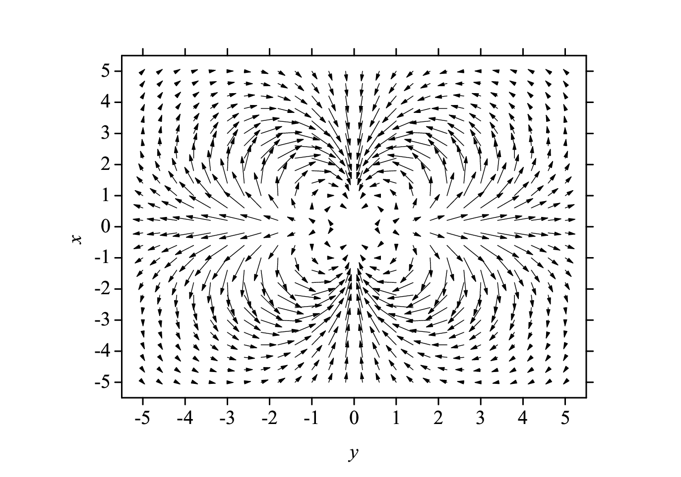
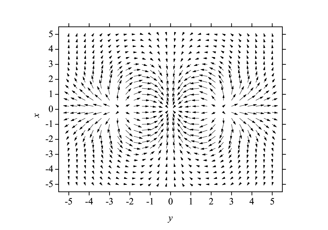
Figure 7: The figures of the arrow plot of 𝒏\bm{n} of the B=3B=3 solutions in the case of the one centered, r0=0r_{0}=0 solution (left) and the three centered, r0∼3.0r_{0}\sim 3.0 solution (right) for μ=0.08\mu=0.08. The length of the arrow is relative to the norm of the vector, i.e. n12+n22\sqrt{n_{1}^{2}+n_{2}^{2}}.

We tried using the following boundary conditions,

F⁡(0,θ)=0,∂rΘ⁡(r,θ)|r=0=0,F⁡(∞,θ)=π,∂rΘ⁡(r,θ)|r=∞=0,for−π2≦θ≦π2\displaystyle F(0,\theta)=0,~~\partial_{r}\Theta(r,\theta)|_{r=0}=0,~~F(\infty,\theta)=\pi,~~\partial_{r}\Theta(r,\theta)|_{r=\infty}=0,~~{\rm for}~~-\frac{\pi}{2}\leqq\theta\leqq\frac{\pi}{2} (12)

and

∂θF⁡(r,θ)|θ=±π2=0,Θ⁡(r,±π2)=±32​π,for​0≦r≦∞.\displaystyle\partial_{\theta}F(r,\theta)|_{\theta=\pm\frac{\pi}{2}}=0,~~\Theta(r,\pm\frac{\pi}{2})=\pm\frac{3}{2}\pi,~~{\rm for}~~0\leqq r\leqq\infty. (13)

Although they are sufficient to get the solutions with axisymmetry (i.e.,the left panel of Fig.1), they are not suited for the symmetry breaking solutions and additional conditions seem to be required to reproduce the results. The reason is that for a critical value of μ\mu, peaks appear and grow at a finite distance from the origin (see Fig.1). These points are singular points where the direction of the component arrow of 𝒏\bm{n} is frustrated. The geometric structure is schematically drawn in Fig.3; one easily see that for r<r0r<r_{0} (here rr is the distance from the origin), the geometry looks like the one center hedgehog, while for r>r0r>r_{0} the arrow winds three times around the origin. We take this property of the solution geometry into account by using the following boundary conditions (12),

∂θF⁡(r,θ)|θ=±π2=0,for​0≦r<r0,r0<r≦∞,\displaystyle\partial_{\theta}F(r,\theta)|_{\theta=\pm\frac{\pi}{2}}=0,~~{\rm for}~~0\leqq r<r_{0},\ r_{0}<r\leqq\infty, (14)
F⁡(r0,±π2)=0\displaystyle F(r_{0},\pm\frac{\pi}{2})=0 (15)

and

Θ⁡(r,±π2)={±π20≦r<r0±32​πr0≦r≦∞\displaystyle\Theta(r,\pm\frac{\pi}{2})=\left\{\begin{array}[]{lrr}\displaystyle\pm\frac{\pi}{2}&0\leqq r<&r_{0}\\ \\ \displaystyle\pm\frac{3}{2}\pi&r_{0}\leqq r\leqq&\infty\end{array}\right.

where r0r_{0} is a constant describing the center distance of the solution constituent solitons. Note that when r0→0r_{0}\to 0 the boundary conditions (14)-(II.1) coincide with the case of the axisymmetry (13). One can easily check that these modified boundary conditions correctly reproduce B=3B=3 (see appendix).

The equations with the appropriate boundary conditions can be solved numerically by the SOR method. In order to get the non-axisymmetric solution, we employ the following procedures. We begin the SOR for a fixed r0r_{0} with following initial conditions which satisfies the boundary behavior of the axisymmetric solutions

F⁡(r,θ)|initial=π⁡(1−e−A​r3),Θ⁡(r,θ)|initial=3​θ.\displaystyle F(r,\theta)|_{\rm initial}=\pi(1-e^{-Ar^{3}}),~~~~\Theta(r,\theta)|_{\rm initial}=3\theta. (20)

For changing r0r_{0}, we repeat the computation and finally reach the true value of r0r_{0} by minimizing the energy par topological charge E/BE/B, which realizes the true boundary condition for the system. In terms of the procedure, we successfully find the non-axisymmetric shape of the solutions.

In Fig.4 we plot a typical E/BE/B as a function of r0r_{0}. In this case, we could choose r0=2.6r_{0}=2.6 as a minimized energy per unit charge. Fig.5 shows a numerical result of the profile functions F⁡(ρ,θ),Θ⁡(ρ,θ)F(\rho,\theta),\Theta(\rho,\theta). In Fig.6, we present the corresponding topological charge density for several potential parameter μ\mu. One easily sees that for increasing values of μ\mu, the peaks grow and a new peak appears at the origin. Note that the F,ΘF,\Theta profiles contain singularities/discontinuities corresponding to the centers of the constituents. In Fig.7 we plot the configurations of 𝒏\bm{n}, i.e., the vectors (n1,n2)(n_{1},n_{2}) on the plane for the case of r0=0.0r_{0}=0.0 and r0∼3.0r_{0}\sim 3.0 which corresponds to minima of the case of μ=0.08\mu=0.08. One easily see that these are perfectly regular.

In Fig.8 we plot the behavior of the deformation parameter Δ\Delta for changing the strength of the potential. For larger μ\mu, the deformation monotonically grows. Note that there is a critical point of the deformation of the solution: for μ∼0.04\mu\sim 0.04, deformed solutions suddenly appear. The error-bar is due to the fact that the results involve a systematic uncertainly for the determination of r0r_{0}.

The solution of the Euler-Lagrange equation should coincide with result of the energy-minimization scheme. In Fig.9, we compare the energy EE and also the energy per topological charge E/BE/B in terms of the SOR and of the SA for the potential parameters μ\mu. Both methods contain uncertainties in several reasons, in particular the SA always tends to underestimate the topological charge as well as the energy. As a result, the energy of the SA is lower value than that of the SOR while the energy per topological charge is slightly higher, but the results are in good agreement within ∼5%\sim 5\%.

For higher charge, solutions breaking the axisymmetry appear even for very small μ\mu.

Refer to caption
Figure 8: The deformation parameter Δ\Delta of the B=3B=3 solution as a function of μ\mu.
Refer to caption
Refer to caption
Figure 9: The comparison of the static energies (left) and the energies per the topological charge (right) of the B=3B=3 solutions for the successive over-relaxation (straight line) and the simulated annealing (dotted line).

II.2 The B=4B=4 solution

The cases with a ℤ2\mathbb{Z}_{2}-symmetry are treated essentially in the same way as in the B=3B=3 case. Therefore, here we concentrate on the case of ℤ3\mathbb{Z}_{3}-symmetry. A typical result of the energy density is shown in Fig. 2.

For the ℤ3\mathbb{Z}_{3}-symmetric case, the equations must be invariant under the transformations

θ→θ+2​π3:F⁡(r,θ)→F⁡(r,θ+2​π3),Θ0​(r,θ)→Θ0​(r,θ+2​π3)\displaystyle\theta\rightarrow\theta+\frac{2\pi}{3}:~~F(r,\theta)\rightarrow F(r,\theta+\frac{2\pi}{3}),~~\Theta_{0}(r,\theta)\rightarrow\Theta_{0}(r,\theta+\frac{2\pi}{3}) (21)

and if we assume that one of the peak is located on the xx-axis (θ=π\theta=\pi), the equations are invariant under the transformations

θ→−θ:F⁡(r,θ)→F⁡(r,−θ),Θ0​(r,θ)→−Θ0​(r,−θ).\displaystyle\theta\rightarrow-\theta:~~F(r,\theta)\rightarrow F(r,-\theta),~~\Theta_{0}(r,\theta)\rightarrow-\Theta_{0}(r,-\theta). (22)

Therefore we perform our numerical calculations on the one third-plane defined as 0≦r≦∞0\leqq r\leqq\infty and −π3≦θ≦π3-\frac{\pi}{3}\leqq\theta\leqq\frac{\pi}{3}. The functions on the whole plane can be estimated in terms of the above symmetry.

We use the following boundary conditions:

F⁡(0,θ)=0,∂rΘ⁡(r,θ)|r=0=0,F⁡(∞,θ)=π,∂rΘ⁡(r,θ)|r=∞=0,for−π3≦θ≦π3\displaystyle F(0,\theta)=0,~~\partial_{r}\Theta(r,\theta)|_{r=0}=0,~~F(\infty,\theta)=\pi,~~\partial_{r}\Theta(r,\theta)|_{r=\infty}=0,~~{\rm for}~~-\frac{\pi}{3}\leqq\theta\leqq\frac{\pi}{3} (23)

and

∂θF⁡(r,θ)|θ=±2​π3=0,Θ⁡(r,±π3)=±4​π3,for​0≦r≦∞\displaystyle\partial_{\theta}F(r,\theta)|_{\theta=\pm\frac{2\pi}{3}}=0,~~\Theta(r,\pm\frac{\pi}{3})=\pm\frac{4\pi}{3},~~{\rm for}~~0\leqq r\leqq\infty (24)

for the axial symmetric solutions and when the constituent soliton centers are located on the line of θ=±π3,π\theta=\pm\frac{\pi}{3},\pi , we take the singularities of the centers into account by imposing

F⁡(0,θ)=0,∂rΘ⁡(r,θ)|r=0=0,F⁡(∞,θ)=π,∂rΘ⁡(r,θ)|r=∞=0,for−π3≦θ≦π3\displaystyle F(0,\theta)=0,~~\partial_{r}\Theta(r,\theta)|_{r=0}=0,~~F(\infty,\theta)=\pi,~~\partial_{r}\Theta(r,\theta)|_{r=\infty}=0,~~{\rm for}~~-\frac{\pi}{3}\leqq\theta\leqq\frac{\pi}{3} (25)
∂θF⁡(r,θ)|θ=±π3=0,for​0≦r<r0,r0<r≦∞,\displaystyle\partial_{\theta}F(r,\theta)|_{\theta=\pm\frac{\pi}{3}}=0,~~{\rm for}~~0\leqq r<r_{0},\ r_{0}<r\leqq\infty, (26)
F⁡(r0,±π3)=0\displaystyle F(r_{0},\pm\frac{\pi}{3})=0 (27)

and

Θ⁡(r,±π3)={±π30≦r<r0±4​π3r0≦r≦∞.\displaystyle\Theta(r,\pm\frac{\pi}{3})=\left\{\begin{array}[]{lrr}\displaystyle\pm\frac{\pi}{3}&0\leqq r<&r_{0}\\ \\ \displaystyle\pm\frac{4\pi}{3}&r_{0}\leqq r\leqq&\infty.\end{array}\right.

Again for r0→0r_{0}\to 0 the boundary conditions reduces to the axisymmetric case.

Refer to caption
Refer to caption
Figure 10: The profiles F⁡(r,θ)F(r,\theta), Θ⁡(r,θ)\Theta(r,\theta) of the B=4B=4 as solutions of the Euler-Lagrange equations with s=2,μ=0.01s=2,\mu=0.01.

Fig.10 shows a numerical result of the profile functions F⁡(ρ,θ),Θ⁡(ρ,θ)F(\rho,\theta),\Theta(\rho,\theta).

III The gravitating baby-Skyrme model in six dimensions

We are now are ready to include gravity to the baby-Skyrme brane model. In this paper, we will focus on the B=3B=3 but the method is straightforwardly extendable to the cases of different BB. We also show the result for B=4B=4 as an example.

The total action for the gravitating baby-Skyrme model in six dimensions is of the form S=Sgrav+SbabyS=S_{\text{grav}}+S_{\text{baby}} with

Sgrav=∫d6​x​−g​(12​χ(6)​R−Λ(6)),S_{\text{grav}}=\int d^{6}x\sqrt{-g}\left(\frac{1}{2\chi_{(6)}}R-\Lambda_{(6)}\right), (32)
Sbaby=∫d6​x​−g​ℒbaby,\displaystyle S_{\text{baby}}=\int d^{6}x\sqrt{-g}{\cal L}_{\text{baby}}, (33)

where Λ(6)\Lambda_{(6)} is the bulk cosmological constant, and χ(6)=8​π​G(6)=8​π/M(6)4\chi_{(6)}=8\pi G_{(6)}=8\pi/M_{(6)}^{4}.

The coefficients κ2,4,0\kappa_{2,4,0} in Eq.(33) are the dimensionful coupling constants in the gravitating baby-Skyrme model with dimensions [Λ(6)]=M6[\Lambda_{(6)}]=M^{6}, [χ(6)]=M−4[\chi_{(6)}]=M^{-4}, [κ2]=M4[\kappa_{2}]=M^{4}, [κ4]=M2[\kappa_{4}]=M^{2} [κ0]=M6[\kappa_{0}]=M^{6}.

III.1 The Ansatz

We consider the case of axial symmetry breaking in the extra dimensions, and we use the following metric ansatz inspired by the Lewis-Papapetrou ansatz in 44-dimensions

d​s2=M2​(ρ,θ)​gμ​ν(4)​d​xμ​d​xν−L2​(ρ,θ)M2​(ρ,θ)​(d​ρ2+ρ2​d​θ2)ds^{2}=M^{2}(\rho,\theta)g_{\mu\nu}^{(4)}dx^{\mu}dx^{\nu}-\frac{L^{2}(\rho,\theta)}{M^{2}(\rho,\theta)}(d\rho^{2}+\rho^{2}d\theta^{2}) (34)

where ρ∈[0,∞)\rho\in[0,\infty) and θ∈[−π,π]\theta\in[-\pi,\pi] are the coordinates associated with the extra dimensions. We further model a cosmological constant on the brane by considering the following form of the four dimensional subspace (described by gμ​ν(4)g_{\mu\nu}^{(4)} in Eq.(34))

d​s(4)2=gμ​ν(4)​d​xμ​d​xν=d​t2−δi​j​e2​H​(t)​d​xi​d​xj.ds_{(4)}^{2}=g_{\mu\nu}^{(4)}dx^{\mu}dx^{\nu}=dt^{2}-\delta_{ij}e^{2H(t)}dx^{i}dx^{j}. (35)

H⁡(t)H(t) is a function of the time coordinate tt which describes the inflation in the four dimensions.

III.2 Field equations of the model

In order to rewrite the system in terms of dimensionless quantities, we define the dimensionless variable

r:=κ2κ4​ρ,ℋ⁡(t):=κ4κ2​H​(t).r:=\sqrt{\frac{\kappa_{2}}{\kappa_{4}}}\,\rho,\;\;\;\mathcal{H}(t):=\sqrt{\frac{\kappa_{4}}{\kappa_{2}}}H(t). (36)

and dimensionless parameters

α:=χ(6)​κ2,β:=Λ(6)​κ4κ22,μ:=κ0​κ4κ22.\displaystyle\alpha:=\chi_{(6)}\kappa_{2},\ \beta:=\Lambda_{(6)}\frac{\kappa_{4}}{\kappa_{2}^{2}},\ \mu:=\kappa_{0}\frac{\kappa_{4}}{\kappa_{2}^{2}}. (37)

After straightforward computations, the Einstein equations reduce to

M2L2​[2​∂r2MM+4​(∂rMM)2+2r​∂rMM+∂r2LL−(∂rLL)2+1r​∂rLL]\displaystyle\frac{M^{2}}{L^{2}}\Bigl[2\frac{\partial_{r}^{2}M}{M}+4\Bigl(\frac{\partial_{r}M}{M}\Bigr)^{2}+\frac{2}{r}\frac{\partial_{r}M}{M}+\frac{\partial_{r}^{2}L}{L}-\Bigl(\frac{\partial_{r}L}{L}\Bigr)^{2}+\frac{1}{r}\frac{\partial_{r}L}{L}\Bigr]
+M2r2​L2​[2​∂θ2MM+4​(∂θMM)2+∂θ2LL−(∂θLL)2]−3ℋ,t2M2=α⁡(τ0−β),\displaystyle\hskip 28.45274pt+\frac{M^{2}}{r^{2}L^{2}}\Bigl[2\frac{\partial_{\theta}^{2}M}{M}+4\Bigl(\frac{\partial_{\theta}M}{M}\Bigr)^{2}+\frac{\partial_{\theta}^{2}L}{L}-\Bigl(\frac{\partial_{\theta}L}{L}\Bigr)^{2}\Bigr]-\frac{3\mathcal{H}_{,t}^{2}}{M^{2}}=\alpha(\tau_{0}-\beta), (38)
M2L2​[2​∂r2MM+4​(∂rMM)2+2r​∂rMM+∂r2LL−(∂rLL)2+1r​∂rLL]\displaystyle\frac{M^{2}}{L^{2}}\Bigl[2\frac{\partial_{r}^{2}M}{M}+4\Bigl(\frac{\partial_{r}M}{M}\Bigr)^{2}+\frac{2}{r}\frac{\partial_{r}M}{M}+\frac{\partial_{r}^{2}L}{L}-\Bigl(\frac{\partial_{r}L}{L}\Bigr)^{2}+\frac{1}{r}\frac{\partial_{r}L}{L}\Bigr]
+M2r2​L2​[2​∂θ2MM+4​(∂θMM)2+∂θ2LL−(∂θLL)2]−2ℋ,t,t+3ℋ,t2M2=α⁡(τ0−β),\displaystyle\hskip 28.45274pt+\frac{M^{2}}{r^{2}L^{2}}\Bigl[2\frac{\partial_{\theta}^{2}M}{M}+4\Bigl(\frac{\partial_{\theta}M}{M}\Bigr)^{2}+\frac{\partial_{\theta}^{2}L}{L}-\Bigl(\frac{\partial_{\theta}L}{L}\Bigr)^{2}\Bigr]-\frac{2\mathcal{H}_{,t,t}+3\mathcal{H}_{,t}^{2}}{M^{2}}=\alpha(\tau_{0}-\beta), (39)
M2L2​[2​(∂rMM)2+4r​∂rMM+4​∂rM​∂rLM​L]\displaystyle\frac{M^{2}}{L^{2}}\Bigl[2\Bigl(\frac{\partial_{r}M}{M}\Bigr)^{2}+\frac{4}{r}\frac{\partial_{r}M}{M}+4\frac{\partial_{r}M\partial_{r}L}{ML}\Bigr]
+M2r2​L2​[4​∂θ2MM+10​(∂θMM)2−4​∂θM​∂θLM​L]−3ℋ,t,t+6ℋ,t2M2=α⁡(τr−β),\displaystyle\hskip 28.45274pt+\frac{M^{2}}{r^{2}L^{2}}\Bigl[4\frac{\partial_{\theta}^{2}M}{M}+10\Bigl(\frac{\partial_{\theta}M}{M}\Bigr)^{2}-4\frac{\partial_{\theta}M\partial_{\theta}L}{ML}\Bigr]-\frac{3\mathcal{H}_{,t,t}+6\mathcal{H}_{,t}^{2}}{M^{2}}=\alpha(\tau_{r}-\beta), (40)
M2L2​[4​∂r2MM+10​(∂rMM)2−4​∂rM​∂rLM​L]\displaystyle\frac{M^{2}}{L^{2}}\Bigl[4\frac{\partial_{r}^{2}M}{M}+10\Bigl(\frac{\partial_{r}M}{M}\Bigr)^{2}-4\frac{\partial_{r}M\partial_{r}L}{ML}\Bigr]
+M2r2​L2​[2​(∂θMM)2+4​∂θM​∂θLM​L]−3ℋ,t,t+6ℋ,t2M2=α⁡(τθ−β),\displaystyle\hskip 28.45274pt+\frac{M^{2}}{r^{2}L^{2}}\Bigl[2\Bigl(\frac{\partial_{\theta}M}{M}\Bigr)^{2}+4\frac{\partial_{\theta}M\partial_{\theta}L}{ML}\Bigr]-\frac{3\mathcal{H}_{,t,t}+6\mathcal{H}_{,t}^{2}}{M^{2}}=\alpha(\tau_{\theta}-\beta), (41)

where we used the notation ℋ,t:=∂tℋ(t)\mathcal{H}_{,t}:=\partial_{t}\mathcal{H}(t) and ℋ,t,t:=∂t2ℋ(t)\mathcal{H}_{,t,t}:=\partial_{t}^{2}\mathcal{H}(t). Let us note that (38) and (39) are the four-dimensional components of the Einstein equation, while (40) and (41) are the extra-dimensional components. The components of the dimensionless energy-momentum (EM) tensor in Eqs.(38)-(41) are given by

τ0=−M22​L2((∂rF)2+sin2F(∂rΘ)2)−M22​r2​L2((∂θF)2+sin2F(∂θΘ)2)−M42​r2​L4sin2F(∂[rF∂θ]Θ)2−μV(𝒏),\displaystyle\tau_{0}=-\frac{M^{2}}{2L^{2}}\bigl((\partial_{r}F)^{2}+\sin^{2}F(\partial_{r}\Theta)^{2}\bigr)-\frac{M^{2}}{2r^{2}L^{2}}\bigl((\partial_{\theta}F)^{2}+\sin^{2}F(\partial_{\theta}\Theta)^{2}\bigr)-\frac{M^{4}}{2r^{2}L^{4}}\sin^{2}F(\partial_{[r}F\partial_{\theta]}\Theta)^{2}-\mu V(\bm{n}), (42)
τr=M22​L2((∂rF)2+sin2F(∂rΘ)2)−M22​r2​L2((∂θF)2+sin2F(∂θΘ)2)+M42​r2​L4sin2F(∂[rF∂θ]Θ)2−μV(𝒏),\displaystyle\tau_{r}=~~~\frac{M^{2}}{2L^{2}}\bigl((\partial_{r}F)^{2}+\sin^{2}F(\partial_{r}\Theta)^{2}\bigr)-\frac{M^{2}}{2r^{2}L^{2}}\bigl((\partial_{\theta}F)^{2}+\sin^{2}F(\partial_{\theta}\Theta)^{2}\bigr)+\frac{M^{4}}{2r^{2}L^{4}}\sin^{2}F(\partial_{[r}F\partial_{\theta]}\Theta)^{2}-\mu V(\bm{n}),
τθ=−M22​L2((∂rF)2+sin2F(∂rΘ)2)+M22​r2​L2((∂θF)2+sin2F(∂θΘ)2)+M42​r2​L4sin2F(∂[rF∂θ]Θ)2−μV(𝒏),\displaystyle\tau_{\theta}=-\frac{M^{2}}{2L^{2}}\bigl((\partial_{r}F)^{2}+\sin^{2}F(\partial_{r}\Theta)^{2}\bigr)+\frac{M^{2}}{2r^{2}L^{2}}\bigl((\partial_{\theta}F)^{2}+\sin^{2}F(\partial_{\theta}\Theta)^{2}\bigr)+\frac{M^{4}}{2r^{2}L^{4}}\sin^{2}F(\partial_{[r}F\partial_{\theta]}\Theta)^{2}-\mu V(\bm{n}),

where ∂[rF∂θ]Θ:=∂rF∂θΘ−∂θF∂rΘ\partial_{[r}F\partial_{\theta]}\Theta:=\partial_{r}F\partial_{\theta}\Theta-\partial_{\theta}F\partial_{r}\Theta.

From (38),(39) one directly sees that the function ℋ⁡(t)\mathcal{H}(t) must be linear in time:

ℋ⁡(t)=ℋ0​t\displaystyle\mathcal{H}(t)=\mathcal{H}_{0}t (43)

where ℋ0\mathcal{H}_{0} is a constant called Hubble parameter. For later convenience, we introduce a dimensionless parameter

γ:=ℋ02=κ4κ2​H02.\displaystyle\gamma:=\mathcal{H}_{0}^{2}=\frac{\kappa_{4}}{\kappa_{2}}H_{0}^{2}. (44)

We finally get the following equations by using a suitable linear combination of (38)-(41)

M2L2​[2​∂r2MM+6​(∂rMM)2+2r​∂rMM]+M2r2​L2​[2​∂θ2MM+6​(∂θMM)2]−6​γM2=α⁡(12​τr+12​τθ−β)\displaystyle\frac{M^{2}}{L^{2}}\Bigl[2\frac{\partial_{r}^{2}M}{M}+6\Bigl(\frac{\partial_{r}M}{M}\Bigr)^{2}+\frac{2}{r}\frac{\partial_{r}M}{M}\Bigr]+\frac{M^{2}}{r^{2}L^{2}}\Bigl[2\frac{\partial_{\theta}^{2}M}{M}+6\Bigl(\frac{\partial_{\theta}M}{M}\Bigr)^{2}\Bigr]-\frac{6\gamma}{M^{2}}=\alpha(\frac{1}{2}\tau_{r}+\frac{1}{2}\tau_{\theta}-\beta) (45)
M2L2​[∂r2LL−(∂rLL)2+1r​∂rLL−2​(∂rMM)2]\displaystyle\frac{M^{2}}{L^{2}}\Bigl[\frac{\partial_{r}^{2}L}{L}-\Bigl(\frac{\partial_{r}L}{L}\Bigr)^{2}+\frac{1}{r}\frac{\partial_{r}L}{L}-2\Bigl(\frac{\partial_{r}M}{M}\Bigr)^{2}\Bigr]
+M2r2​L2​[∂θ2LL−(∂θLL)2−2​(∂θMM)2]+3​γM2=α⁡(τ0−12​τr−12​τθ).\displaystyle\hskip 113.81102pt+\frac{M^{2}}{r^{2}L^{2}}\Bigl[\frac{\partial_{\theta}^{2}L}{L}-\Bigl(\frac{\partial_{\theta}L}{L}\Bigr)^{2}-2\Bigl(\frac{\partial_{\theta}M}{M}\Bigr)^{2}\Bigr]+\frac{3\gamma}{M^{2}}=\alpha(\tau_{0}-\frac{1}{2}\tau_{r}-\frac{1}{2}\tau_{\theta}). (46)

For the matter fields, the equations are given by

M2L2​{∂r2F+(4​∂rMM+1r)​∂rF−12​sin⁡2​F​(∂rΘ)2}+M2r2​L2​(∂θ2F+4​∂θMM​∂θF−12​sin⁡2​F​(∂θΘ)2)\displaystyle\frac{M^{2}}{L^{2}}\Bigl\{\partial_{r}^{2}F+\Bigl(4\frac{\partial_{r}M}{M}+\frac{1}{r}\Bigr)\partial_{r}F-\frac{1}{2}\sin 2F(\partial_{r}\Theta)^{2}\Bigr\}+\frac{M^{2}}{r^{2}L^{2}}\Bigl(\partial_{\theta}^{2}F+4\frac{\partial_{\theta}M}{M}\partial_{\theta}F-\frac{1}{2}\sin 2F(\partial_{\theta}\Theta)^{2}\Bigr)
+M4r2​L4sin2F[{(6∂rMM−2∂rLL−1r)∂θΘ−(6∂θMM−2∂θLL)∂rΘ}(∂[rF∂θ]Θ)\displaystyle+\frac{M^{4}}{r^{2}L^{4}}\sin^{2}F\Bigl[\Bigl\{\Bigl(6\frac{\partial_{r}M}{M}-2\frac{\partial_{r}L}{L}-\frac{1}{r}\Bigr)\partial_{\theta}\Theta-\Bigl(6\frac{\partial_{\theta}M}{M}-2\frac{\partial_{\theta}L}{L}\Bigr)\partial_{r}\Theta\Bigr\}(\partial_{[r}F\partial_{\theta]}\Theta)
+∂r2F(∂θΘ)2+∂θ2F(∂rΘ)2+(∂{rF∂θ}Θ)∂r​θΘ\displaystyle\hskip 28.45274pt+\partial_{r}^{2}F(\partial_{\theta}\Theta)^{2}+\partial_{\theta}^{2}F(\partial_{r}\Theta)^{2}+(\partial_{\{r}F\partial_{\theta\}}\Theta)\partial_{r\theta}\Theta
−(∂r2Θ∂θΘ∂θF+∂θ2Θ∂rΘ∂rF+2∂r​θF∂θΘ∂rΘ)+cotF(∂{rF∂θ}Θ)2]−μ∂V∂F=0\displaystyle\hskip 28.45274pt-(\partial_{r}^{2}\Theta\partial_{\theta}\Theta\partial_{\theta}F+\partial_{\theta}^{2}\Theta\partial_{r}\Theta\partial_{r}F+2\partial_{r\theta}F\partial_{\theta}\Theta\partial_{r}\Theta)+\cot F(\partial_{\{r}F\partial_{\theta\}}\Theta)^{2}\Bigr]-\mu\frac{\partial V}{\partial F}=0 (47)
M2L2{∂r2Θ+(4∂rMM+1r)∂rΘ+2cotF∂rF∂rΘ}+M2r2​L2(∂θ2Θ+4∂θMM∂θΘ+2cotF∂θF∂θΘ)\displaystyle\frac{M^{2}}{L^{2}}\Bigl\{\partial_{r}^{2}\Theta+\Bigl(4\frac{\partial_{r}M}{M}+\frac{1}{r}\Bigr)\partial_{r}\Theta+2\cot F\partial_{r}F\partial_{r}\Theta\Bigl\}+\frac{M^{2}}{r^{2}L^{2}}\Bigl(\partial_{\theta}^{2}\Theta+4\frac{\partial_{\theta}M}{M}\partial_{\theta}\Theta+2\cot F\partial_{\theta}F\partial_{\theta}\Theta\Bigr)
−M4r2​L4[{(6∂rMM−2∂rLL−1r)∂θF−(6∂θMM−2∂θLL)∂rF}(∂[rF∂θ]Θ)\displaystyle-\frac{M^{4}}{r^{2}L^{4}}\Bigl[\Bigl\{\Bigl(6\frac{\partial_{r}M}{M}-2\frac{\partial_{r}L}{L}-\frac{1}{r}\Bigr)\partial_{\theta}F-\Bigl(6\frac{\partial_{\theta}M}{M}-2\frac{\partial_{\theta}L}{L}\Bigr)\partial_{r}F\Bigr\}(\partial_{[r}F\partial_{\theta]}\Theta)
+∂r2Θ(∂θF)2+∂θ2Θ(∂rF)2+(∂{rF∂θ}Θ)∂r​θF\displaystyle\hskip 28.45274pt+\partial_{r}^{2}\Theta(\partial_{\theta}F)^{2}+\partial_{\theta}^{2}\Theta(\partial_{r}F)^{2}+(\partial_{\{r}F\partial_{\theta\}}\Theta)\partial_{r\theta}F
−(∂r2F∂θF∂θΘ+∂θ2F∂rF∂rΘ+2∂r​θΘ∂θF∂rF)]=0\displaystyle\hskip 42.67912pt-(\partial_{r}^{2}F\partial_{\theta}F\partial_{\theta}\Theta+\partial_{\theta}^{2}F\partial_{r}F\partial_{r}\Theta+2\partial_{r\theta}\Theta\partial_{\theta}F\partial_{r}F)\Bigr]=0 (48)

where ∂{rF∂θ}Θ:=∂rF∂θΘ+∂θF∂rΘ\partial_{\{r}F\partial_{\theta\}}\Theta:=\partial_{r}F\partial_{\theta}\Theta+\partial_{\theta}F\partial_{r}\Theta and ∂r​θ:=∂r∂θ\partial_{r\theta}:=\partial_{r}\partial_{\theta}.

Refer to caption
Refer to caption
Figure 11: The profiles of the functions F⁡(r,θ)F(r,\theta) (left), Θ⁡(r,θ)\Theta(r,\theta) (right) with μ=0.08,α=0.005,β=0.00,γ=0.00\mu=0.08,\alpha=0.005,\beta=0.00,\gamma=0.00.
Refer to caption
Refer to caption
Refer to caption
Refer to caption
Figure 12: The metrics L⁡(r,θ),M⁡(r,θ)L(r,\theta),M(r,\theta) for β=0.05\beta=0.05 (left) and β=−0.05\beta=-0.05 (right). The remaining parameters are set to μ=0.08,α=0.005,γ=0.00\mu=0.08,\alpha=0.005,\gamma=0.00.

A useful quantity for the gravity-side is the rescaled Ricci scalar which is given by

R⁡(r,θ)\displaystyle R(r,\theta) =\displaystyle= M2L2​[6​∂r2MM+14​(∂rMM)2+6r​∂rMM+2​∂r2LL−2​(∂rLL)2+2r​∂rLL]\displaystyle\frac{M^{2}}{L^{2}}\Bigl[6\frac{\partial_{r}^{2}M}{M}+14\Bigl(\frac{\partial_{r}M}{M}\Bigr)^{2}+\frac{6}{r}\frac{\partial_{r}M}{M}+2\frac{\partial_{r}^{2}L}{L}-2\Bigl(\frac{\partial_{r}L}{L}\Bigr)^{2}+\frac{2}{r}\frac{\partial_{r}L}{L}\Bigr] (49)
+\displaystyle+ M2r2​L2​[6​∂θ2MM+14​(∂θMM)2+2​∂θ2LL−2​(∂θLL)2]−12​γM2.\displaystyle\frac{M^{2}}{r^{2}L^{2}}\Bigl[6\frac{\partial_{\theta}^{2}M}{M}+14\Bigl(\frac{\partial_{\theta}M}{M}\Bigr)^{2}+2\frac{\partial_{\theta}^{2}L}{L}-2\Bigl(\frac{\partial_{\theta}L}{L}\Bigr)^{2}\Bigr]-\frac{12\gamma}{M^{2}}\,.

III.3 Boundary conditions

For the ℤ2\mathbb{Z}_{2}-symmetry, the Einstein equations (38)-(42), and the matter field equations (47),(48) must be invariant under the transformations

θ↔θ+π:F⁡(r,θ)→F⁡(r,θ+π),Θ0​(r,θ)→Θ0​(r,θ+π),M⁡(r,θ)↔M⁡(r,θ+π),L⁡(r,θ)↔L⁡(r,θ+π)\displaystyle\theta\leftrightarrow\theta+\pi:~~F(r,\theta)\rightarrow F(r,\theta+\pi),~~\Theta_{0}(r,\theta)\rightarrow\Theta_{0}(r,\theta+\pi),~~M(r,\theta)\leftrightarrow M(r,\theta+\pi),~~L(r,\theta)\leftrightarrow L(r,\theta+\pi)~~ (50)

and when we set θ=0\theta=0 as the axis of symmetry, the equations mast be invariant under the transformations

θ↔−θ:F⁡(r,θ)→F⁡(r,−θ),Θ0​(r,θ)→−Θ0​(r,−θ),M⁡(r,θ)↔M⁡(r,−θ),L⁡(r,θ)↔L⁡(r,−θ).\displaystyle\theta\leftrightarrow-\theta:~~F(r,\theta)\rightarrow F(r,-\theta),~~\Theta_{0}(r,\theta)\rightarrow-\Theta_{0}(r,-\theta),~~M(r,\theta)\leftrightarrow M(r,-\theta),~~L(r,\theta)\leftrightarrow L(r,-\theta). (51)

Thus as in the case of non gravitation, it is sufficient to restrict the integration domain to the half-plane defined by 0≦r≦∞0\leqq r\leqq\infty and −π2≦θ≦π2-\frac{\pi}{2}\leqq\theta\leqq\frac{\pi}{2}. For the matter fields, we employ the boundary conditions (12) and (14)-(II.1).

For the metric fields, regularity at the core of the brane leads to the following conditions

M⁡(0,θ)=1​∂rM⁡(r,θ)|r=0=0;L⁡(0,θ)=1,∂rL⁡(r,θ)|r=0=0,for−π2≦θ≦π2.\displaystyle\hskip 0.0ptM(0,\theta)=1~~\partial_{r}M(r,\theta)|_{r=0}=0;~~L(0,\theta)=1,~~\partial_{r}L(r,\theta)|_{r=0}=0,~~{\rm for}~~-\frac{\pi}{2}\leqq\theta\leqq\frac{\pi}{2}. (52)

Thus it is likely that the solutions satisfy the following additional boundary conditions

∂θM⁡(r,θ)|θ=±π2=0,∂θL⁡(r,θ)|θ=±π2=0,for​0≦r≦∞.\displaystyle\partial_{\theta}M(r,\theta)|_{\theta=\pm\frac{\pi}{2}}=0,~~\partial_{\theta}L(r,\theta)|_{\theta=\pm\frac{\pi}{2}}=0,~~{\rm for}~~0\leqq r\leqq\infty. (53)

Note that we do not need to impose any conditions for the metrics about r0r_{0} because the local spatial structure of the brane is described by only the matter fields.

III.4 The potential

As we already mentioned, in [23] the authors have introduced a two parameters class of potential

V=μ​(1+n3)s0≤s≤4.\displaystyle V=\mu(1+n_{3})^{s}~~~~0\leq s\leq 4. (54)

In the original approach, the authors used dimensionful parameters (which is essentially our κ4/κ2\kappa_{4}/\kappa_{2}) denoted by κ2\kappa^{2} and minimized the energy for changing values of s,κ2s,\kappa^{2} with fixed μ\mu. The main difference in our analysis is that we vary the parameters of the potential, i.e. μ\mu and successively solve the equations instead of minimizing the energy.

IV Numerical results

In [20], we have done the analysis for the same model but have assumed axisymmetry from the start. In this case the problem reduces to a system of coupled ordinary differential equations. In the present case we have to treat the four coupled partial differential equations (38)-(48) with the boundary conditions (12),(14)-(15) by using the SOR method.

We use the following form

F⁡(r,θ)|initial:=π⁡(1−e−A​r3),Θ⁡(r,θ)|initial:=3​θ\displaystyle F(r,\theta)|_{\rm initial}:=\pi(1-e^{-Ar^{3}}),~~~~\Theta(r,\theta)|_{\rm initial}:=3\theta
M⁡(r,θ)|initial=L⁡(r,θ)|initial=1\displaystyle\hskip 28.45274ptM(r,\theta)|_{\rm initial}=L(r,\theta)|_{\rm initial}=1 (55)

as the initial profile of the relaxation scheme.

Note that the conditions we use, together with the initial profile (55) leads to axisymmetric solution. However, when the deformation is relatively small, they are approximatively consistent with the boundary conditions of the non-axisymmetric case. Thus, we begin with r0=0r_{0}=0 and find the solution. By using this result as a initial profile, the computation for the small finite r0r_{0} is performed. We repeat the procedure until we get the solutions for sufficient large value of r0r_{0}. For the continuous change of r0r_{0}, we can find minimum of the energy per topological charge. Since the true solution should exhibits the minimum energy per charge, we employ the r0r_{0} corresponding to the minimum energy per charge for the boundary conditions.

Since the boundary conditions for the metrics are imposed only at the origin, the Einstein equations essentially are the initial value problem. Usually it is not straightforward to adapt the SOR to the problem. Thus we employ the following procedure. We put an initial guess of the form of L,ML,M at the infinity and solve the equations for that condition. If the condition is inappropriate, the solution surely exhibits the non-trivial singularity at some location, then we explore the proper boundary condition until such singular behavior disappears.

In Fig.11 we show a solution for F,ΘF,\Theta. The metric functions L,ML,M are shown in Fig.12 for both sign of the cosmological constant β\beta. We plot the scalar curvature corresponding to the solutions in Fig.13. In both cases, there are two distinct peaks together with the remaining slight ridge. The result for the μ=0.08\mu=0.08; if we choose larger value of μ\mu, the peaks grow and finally end up in three independent peaks corresponding to the energy density of the baby-skyrmion.

The Ricci scalar for a typical solution with the ℤ3\mathbb{Z}_{3} symmetry is presented in Fig.14. We clearly see three distinct peaks and for larger value of μ\mu, the fourth peak grows at the origin until we finally get a four-centered solution.

Refer to caption
Refer to caption

β=0.05\beta=0.05                   β=−0.05\beta=-0.05

Figure 13: The Ricci scalar curvature of the B=3B=3 solutions for α=0.005,γ=0.0\alpha=0.005,\gamma=0.0 .

V Summary

In this paper, we have obtained the non-axisymmetric brane solutions in the B=3,4B=3,4 baby-Skyrme model with the old-baby potential. We treated the problem in two steps: we first computed the solution using the SA in order to gain intuition on the boundary conditions. Then we solved the four coupled partial differential equations by using the standard SOR by using suitable boundary conditions. The axial symmetry breaks to ℤ2\mathbb{Z}_{2} symmetry and the deformation is a one-parameter family of the strength of the potential μ\mu.

Recently the authors have found at a related model with the present study that there are holomorphic solutions for special choice of the potentials [28, 29]. The potentials are a class of old-baby potential for B=1B=1 while for all other BB they become a class of new-baby. Furthermore, the axisymmetry is a good symmetry for the new-baby potentials while for the old-baby the symmetry is inevitably broken. The most crucial thing for the deformation is thus whether the value of the potential at the origin is finite or not.

Study of the linear stability of the present model has been done in [20] within the assumption of the axial symmetry. Apart from the axial symmetry, we also need to take into account the fluctuation of Θ\Theta. It seems straightforward but surely cumbersome. For the level of the classical solution, our solution is stable for the variation of the size moduli (see Fig.4), so we expect that our solution will be stable against any general perturbation as well.

Of course there are several possibilities of the potential for obtaining the anisotropic solutions. For example, in [27] the authors introduced a more sophisticated potential V=|1−(n1+i​n2)N|2​(1−n3)V=|1-(n_{1}+in_{2})^{N}|^{2}(1-n_{3}) (with the integer N≧2N\geqq 2). However the potential is essentially of old-type and the solution tends to split the number of BB constituents. An interesting feature of such models is the fine structure: the zero of the potential are at the infinity (F=0)(F=0) as well as the points F=π2F=\frac{\pi}{2} and Θ=n​πN\Theta=\frac{n\pi}{N} (nn:integer). As a result, the solution split BB component where each has N​BNB peaks.

An intersting question raised by this work is to see the effects of the the spatial structure of the branes on the mass of the brane localized fermions (quarks, leptons). The fermions coupled with the baby-skyrmions with Yukawa-coupling exhibit non-trivial doubly degenerated plus isolated states which could be identified as three generations of the quarks/leptons. The model has weak isospin symmetry and the isodoublet of the quarks are degenerate. We expect that the brane slightly deforms from the axisymmetry and reproduce the slight splitting the mass of the first and second levels [17]. Now we got the intuition that the level splitting of the generations is owed by the coupling constant of the old-baby potential μ\mu. More thorough analysis of the property of the localized fermions in these funny structures of the brane will be certainly very interesting.

Refer to caption
Figure 14: The Ricci scalar curvature of the B=4B=4 for α=0.005,β=0.0,μ=0.01,s=2\alpha=0.005,\beta=0.0,\mu=0.01,s=2.

Appendix A Topological charge

The topological charge defined by (2) is easily computed for the boundary conditions (12), (14)-(II.1). From (8)

B\displaystyle B =\displaystyle= −12​π∫−π2π2dθ∫0∞dr[∂r(cosF∂θΘ)−∂θ(cosF∂rΘ)]\displaystyle-\frac{1}{2\pi}\int_{-\frac{\pi}{2}}^{\frac{\pi}{2}}d\theta\int_{0}^{\infty}dr~\bigl[\partial_{r}(\cos F\partial_{\theta}\Theta)-\partial_{\theta}(\cos F\partial_{r}\Theta)\bigr] (56)
=\displaystyle= −12​π∫−π2π2dθ[cosF∂θΘ]0∞+12​π∫0∞dr[cosF∂rΘ]−π2π2\displaystyle-\frac{1}{2\pi}\int_{-\frac{\pi}{2}}^{\frac{\pi}{2}}d\theta~\bigl[\cos F\partial_{\theta}\Theta\bigr]_{0}^{\infty}+\frac{1}{2\pi}\int_{0}^{\infty}dr~\bigl[\cos F\partial_{r}\Theta\bigr]_{-\frac{\pi}{2}}^{\frac{\pi}{2}}
=\displaystyle= −12​π∫−π2π2dθ(cosF|r=∞∂θΘ|r=∞−cosF|r=0∂θΘ|r=0)\displaystyle-\frac{1}{2\pi}\int_{-\frac{\pi}{2}}^{\frac{\pi}{2}}d\theta~\bigl(\cos F|_{r=\infty}\partial_{\theta}\Theta|_{r=\infty}-\cos F|_{r=0}\partial_{\theta}\Theta|_{r=0}\bigr)
+12​π∫0∞dr(cosF|θ=π2∂rΘ|θ=π2−cosF|θ=−π2∂rΘ|θ=−π2)\displaystyle+\frac{1}{2\pi}\int_{0}^{\infty}dr~\bigl(\cos F|_{\theta=\frac{\pi}{2}}\partial_{r}\Theta|_{\theta=\frac{\pi}{2}}-\cos F|_{\theta=-\frac{\pi}{2}}\partial_{r}\Theta|_{\theta=-\frac{\pi}{2}}\bigr)
=\displaystyle= −12​π​((−1)⋅3​π−1⋅π)+12​π​(1⋅π−1⋅(−π))\displaystyle-\frac{1}{2\pi}\bigl((-1)\cdot 3\pi-1\cdot\pi\bigr)+\frac{1}{2\pi}\bigl(1\cdot\pi-1\cdot(-\pi)\bigr)
=\displaystyle= 3\displaystyle 3

where we used the relation ±1π∂rΘ|θ=±π2=δ(r−r0)\pm\frac{1}{\pi}\partial_{r}\Theta|_{\theta=\pm\frac{\pi}{2}}=\delta(r-r_{0}).

References

  • [1] S. Weinberg, Rev. Mod. Phys, 61 (1989) 1.
  • [2] G. Dvali, G. Gabadadze and M. Shifman, Phys. Rev. D 67 (2003) 044020.
  • [3] L. Randall and R. Sundrum, Phys. Rev. Lett. 83, 3370 (1999) [arXiv:hep-ph/9905221].
  • [4] L. Randall and R. Sundrum, Phys. Rev. Lett. 83, 4690 (1999) [arXiv:hep-th/9906064].
  • [5] A. G. Cohen and D. B. Kaplan, Phys. Lett. B 470, 52 (1999) [arXiv:hep-th/9910132].
  • [6] R. Gregory, Phys. Rev. Lett. 84, 2564 (2000) [arXiv:hep-th/9911015].
  • [7] T. Gherghetta and M. E. Shaposhnikov, Phys. Rev. Lett. 85, 240 (2000) [arXiv:hep-th/0004014].
  • [8] M. Giovannini, H. Meyer and M. E. Shaposhnikov, Nucl. Phys. B 619, 615 (2001) [arXiv:hep-th/0104118].
  • [9] C. Ringeval, P. Peter and J. P. Uzan, Phys. Rev. D 71, 104018 (2005) [arXiv:hep-th/0301172].
  • [10] E. Roessl and M. Shaposhnikov, Phys. Rev. D 66, 084008 (2002) [arXiv:hep-th/0205320].
  • [11] T. H. R. Skyrme, Proc. Roy. Soc. Lond. A 260 (1961) 127.
  • [12] G. S. Adkins, C. R. Nappi and E. Witten, Nucl. Phys. B 228, 552 (1983).
  • [13] R. A. Leese, M. Peyrard and W. J. Zakrzewski, Nonlinearity 3, 773 (1990).
  • [14] B. M. A. Piette, B. J. Schroers and W. J. Zakrzewski, Z. Phys. C 65, 165 (1995) [arXiv:hep-th/9406160].
  • [15] A. E. Kudryavtsev, B. Piette and W. J. Zakrzewski, Eur. Phys. J. C 1, 333 (1998) [arXiv:hep-th/9611217].
  • [16] A. E. Kudryavtsev, B. M. A. Piette and W. J. Zakrzewski, Nonlinearity 11, 783 (1998) [arXiv:hep-th/9709187].
  • [17] Y. Kodama, K. Kokubu and N. Sawado, Phys. Rev. D 79, 065024 (2009) [arXiv:0812.2638 [hep-th]].
  • [18] Y. Brihaye, T. Delsate and B. Hartmann, Phys. Rev. D 74, 044015 (2006) [arXiv:hep-th/0602172].
  • [19] Y. Brihaye and T. Delsate, Class. Quant. Grav. 24, 1279-1292 (2007) [arXiv:gr-qc/0605039]
  • [20] Y. Brihaye, T. Delsate, Y. Kodama, N. Sawado, Phys. Rev. D82, 106002 (2010). [arXiv:1007.0736 [hep-th]].
  • [21] T. Delsate and N. Sawado, Phys. Rev. D 85, 065025 (2012) [arXiv:1112.2714 [gr-qc]].
  • [22] M. F. Atiyah, V. K. Patodi and I. M. Singer, Math. Proc. Cambridge Phil. Soc. 79, 71 (1976).
  • [23] I. Hen and M. Karliner, Nonlinearity 21, 399 (2008) [arXiv:0710.3939 [hep-th]].
  • [24] M. Hale, O. Schwindt and T. Weidig, Phys. Rev. E 62, 4333 (2000) [arXiv:hep-th/0002058].
  • [25] “Numerical Recipes in C: The Art of Scientific Computing”, Saul A.Teukolsky,William H.Press,William T,Vetterling (Cambridge University Press, UK, 1988). http://www.nr.com/oldverswitcher.html
  • [26] R. S. Ward, hep-th/0307036.
  • [27] J. Jaykka, M. Speight and P. Sutcliffe, Proc. Roy. Soc. Lond. A 468, 1085 (2012) [arXiv:1106.1125 [hep-th]].
  • [28] L. A. Ferreira, J. Jaykka, N. Sawado and K. Toda, Phys. Rev. D 85, 105006 (2012) [arXiv:1112.1085 [hep-th]].
  • [29] L. A. Ferreira, M. Hayasaka, J. Jaykka, N. Sawado and K. Toda, J.Phys.A, in preparation.