Spin evolution of supermassive black holes and galactic nuclei
Abstract
The spin angular momentum of a supermassive black hole (SBH) precesses due to torques from orbiting stars, and the stellar orbits precess due to dragging of inertial frames by the spinning hole. We solve the coupled post-Newtonian equations describing the joint evolution of and the stellar angular momenta in spherical, rotating nuclear star clusters. In the absence of gravitational interactions between the stars, two evolutionary modes are found: (1) nearly uniform precession of about the total angular momentum vector of the system; (2) damped precession, leading, in less than one precessional period, to alignment of with the angular momentum of the rotating cluster. Beyond a certain distance from the SBH, the time scale for angular momentum changes due to gravitational encounters between the stars is shorter than spin-orbit precession times. We present a model, based on the Ornstein-Uhlenbeck equation, for the stochastic evolution of star clusters due to gravitational encounters and use it to evaluate the evolution of in nuclei where changes in the are due to frame dragging close to the SBH and to encounters farther out. Long-term evolution in this case is well described as uniform precession of the SBH about the cluster’s rotational axis, with an increasingly important stochastic contribution when SBH masses are small. Spin precessional periods are predicted to be strongly dependent on nuclear properties, but typical values are yr for low-mass SBHs in dense nuclei, yr for SBH masses , and yr for the most massive SBHs. We compare the evolution of SBH spins in stellar nuclei to the case of torquing by an inclined, gaseous accretion disk.
pacs
Valid PACS appear hereI Introduction
An accretion disk fed by gas whose angular momentum is misaligned with that of the central supermassive black hole (SBH) will experience Lense-Thirring [1] precession. Viscous torques near the SBH align the gas with the SBH equatorial plane [2]; farther out, the gas remains inclined, producing a constant torque that causes the SBH spin axis to precess. Such precession has been invoked as an explanation for changes in the direction of radio jets in active galaxies [3, 4]. Continued accretion of gas from a misaligned plane will eventually reorient the SBH, although the time required for realignment is uncertain [5].
Accretion disks are believed to be associated with only a small fraction of SBHs. Here we consider the more generic, and perhaps simpler, case of a rotating SBH embedded in a nuclear cluster of stars or stellar remnants. If the cluster has a net angular momentum that is misaligned with the SBH spin, a mutual torque will be exerted between stars and SBH, even if the spatial distribution of the stars is precisely spherical.
In the simplest such model, the stars move independently of each other. Differential precession (“phase mixing”) will nevertheless cause stellar orbits near the SBH to distribute their angular momentum vectors uniformly about the spin , decreasing the torque that they exert on the hole. The angular momentum associated with stars farther out can remain misaligned, leading to a forced precession of the SBH, similar to what occurs in the case of misaligned accretion disks.
By solving the coupled post-Newtonian equations describing a spinning SBH and a rotating cluster, we verify that such an outcome is possible, at least starting from certain initial conditions. However we find a second evolutionary mode as well, in which differential precession causes the inner system to reach alignment with the total (spin plus orbital) angular momentum, resulting in a steady state with no subsequent precession of the hole.
Stars also interact with each other gravitationally; these encounters lead to changes in stellar angular momenta, on time scales that can be short compared with Lense-Thirring times. Unlike changes due to frame-dragging, evolution of the due to encounters is essentially random. There is a region near the SBH, the “sphere of rotational influence,” in which encounter times are long compared with frame-dragging times. Within this region, stellar orbits precess uniformly, while outside of it, changes in the are due primarly to encounters and are random. The size of this sphere varies from pc in the nuclei of galaxies like the Milky Way, to pc in nuclei containing the most massive SBHs. We develop a stochastic model for the evolution of that includes the effects of encounters on the . In this model, net alignment of the stellar angular momena with the SBH spin is less efficient, and the SBH typically continues to precess about the mean of the stellar cluster, although its instantaneous precession rate can vary stochastically due to the stochastically changing .
Evolution of SBH spins to due torquing from stars has many parallels with evolution due to torquing from an accretion disk, surprisingly so given that one process is energy-conserving and the other is dissipative. We compare and contrast the two sorts of evolution in the “Discussion” section, where we also summarize observational and theoretical evidence for nuclear rotation, and discuss the implications of our results for the experimental determination of black hole spins.
Throughout this paper we ignore the contribution of stellar captures to the evolution of .
II Spin-orbit equations
A Kerr black hole of mass has gravitational radius given by
| (1) |
and spin angular momentum , which we write in terms of the dimensionless spin parameter as
| (2) |
To lowest post-Newtonian (PN) order, the spin evolves (precesses) in response to torques from orbiting stars according to [6]
| (3) |
where is the mass of the ’th star, whose instantaneous position and velocity relative to the SBH (assumed fixed at the origin) are , and . Eq. (3) is invariant to the choice of spin supplementarity condition [6]. It can be written in the equivalent form
| (4) |
where
| (5) |
is the Newtonian angular momentum of the ’th star.
We are mainly interested in changes that take place on time scales long compared with stellar orbital periods, , where
| (6) |
Here is the orbital semimajor axis and mpc pc. Accordingly, each of the terms on the right hand side of Eq. (4) can be averaged over the unperturbed (Keplerian) orbit, whose semimajor axis and eccentricity are and . Using
| (7) |
and fixing during the averaging, the spin evolution equation becomes
| (8a) | |||||
| (8b) | |||||
Henceforth averaging over the Keplerian motion will be understood unless otherwise indicated.
Stellar orbits also precess in response to frame-dragging torques from the spinning SBH. Working again to lowest PN order and averaging over the unperturbed motion yields the standard expression for the Lense-Thirring [1] precession:
| (9a) | |||||
| (9b) | |||||
For fixed , precession described by Eq. (9) has the form of uniform advance of the line of nodes, the latter defined as the intersection of the orbital plane with the equatorial plane of the SBH. We denote the nodal angle by ; thus in the orbit-averaged approximation, . Orbits also experience precession of the argument of periastron due to both the Schwarzschild and Kerr components of the SBH metric, but such precession leaves the unchanged.
In the absence of interactions between stars, the coupled equations (8), (9) determine the joint evolution of the SBH spin and the stellar angular momenta. Conserved quantities include the total angular momentum of the system:
| (10) |
as well as
| (11a) | |||||
| (11b) | |||||
Neither , nor is conserved. However conservation of and implies
| (12) |
Consider the case in which all stars have the same and ; for instance, the orbits could lie in a circular ring. There is no differential precession, and Eqs. (8), (9) can be written
| (13) |
where
| (14a) | |||||
| (14b) | |||||
In this special case, is conserved, and both and precess with frequency about the fixed vector . The controlling parameter is . If , and precesses about the fixed SBH spin vector at the Lense-Thirring rate; while if , and precesses about the fixed angular momentum vector of the stars with frequency .
This simple model might apply to the “clockwise stellar disk” at the center of the Milky Way, which has a mass , radius pc, and mean orbital eccentricity [7, 8, 9]. Setting [10], the implied is
| (15) |
consistent within the uncertainties with unity even if is as large as . Evidently, the stars in this disk torque the SBH about as much as they are torqued by it. The mutual precession time is
| (16) |
much longer than the yr age of the disk inferred from the properties of its stars, and also long compared with other physical processes that are likely to alter the stellar orbits (as discussed in more detail below). Nevertheless, this example demonstrates that identified structures near the Galactic center SBH can easily contain a net orbital angular momentum that exceeds .
The distribution of stars at distances pc from Sgr A⋆ is poorly constrained [11, 12, 13], but the total stellar mass in this region is almost certainly large compared with the associated with the clockwise disk. Given the strong () radial dependence of the frame-dragging torques, even a modest degree of net circulation of the stars in this region could therefore induce a precession of the SBH on time scales very short compared with the time of Eq. (16).
We emphasize that there is no need for the torquing stars to lie in a geometrically flattened structure: according to Eqs. (8), all that is needed is a non-random orientation of the orbital angular momentum vectors, which occurs even in a precisely spherical nucleus if there is a preferred sense of orbital circulation.
In general, different stars will have different and , implying different rates of nodal precession. Close enough to the SBH, orbital precession times will be short compared with the precessional period of the SBH, and the orbits will tend to distribute their angular momentum vectors uniformly about the instantaneous . The net torque from these stars will then fall essentially to zero, and continued precession of the SBH will be driven by stars farther out. We expect the radius separating stars in these two regions to be roughly the radius containing a total stellar angular momentum equal to . We estimate that radius in the following section, after first presenting observationally motivated models for stellar nuclei.
III Spherical nuclei
Most of the distributed mass at distances pc from the Milky Way SBH is believed to be in the form of stars much older than the stars in the clockwise disk. The spatial distribution of these stars is believed to be approximately spherical [14], with at least a modest degree of circulation [15, 12].
A simple model for the distribution of mass near the center of a spherical galaxy is
| (17) |
Near the SBH (but not so near that relativistic corrections are required), the gravitational potential is
| (18) |
and orbits can be characterized by their semimajor axes and eccentricities, as in the previous section. If the stellar velocity distribution is assumed to be isotropic and stationary, and if stars are distributed along orbits uniformly with respect to mean anomaly, the joint distribution of and that generates the density (17) is
| (19) |
The relation between , and is easily shown to be
| (20) |
where is the stellar mass, assumed the same for all stars. Values of less than are not achievable if the velocity distribution is isotropic [16]; we do not consider that possibility here, and in the modelling that follows, will be restricted to the range .
The relations (18) - (20) are valid at radii smaller than the SBH influence radius , customarily defined as the radius enclosing a stellar mass equal to :
| (21) |
A spherical cluster will exhibit net rotation if unequal numbers of stars (at each and , say) circulate in a clockwise vs. counter-clockwise sense about some axis. For instance, if one-half of the orbits in a spherical cluster with initially isotropically-distributed velocities have their velocity vectors reversed such that all angular momentum vectors point toward the same half-sphere, the total angular momentum of the ensemble will be . Henceforth we characterize the net rotation of a spherical cluster by the factor , defined as the fraction of orbits that have been “flipped” in this way; and is assumed to be independent of and .
Characterizing the rotation in this way is “conservative,” in the sense that a geometrically flattened nuclear cluster (e.g. a disk), or a spherical cluster consisting of only circular orbits (an “Einstein cluster” [17]), can have a larger net angular momentum for the same radial distribution of mass.

Observed galaxies appear to fall into one of two classes in terms of the parameters that define their stellar distribution at [18]. Massive spheroids – elliptical galaxies, or the bulges of spiral galaxies – with total luminosities greater than have “cores,” regions of size where the stellar density rises slowly toward the SBH. In these galaxies, the observed, mean relation between and is approximately [19]
| (22) |
and the index that defines the central density increase varies from at the highest luminosities to or at the low-luminosity end of the range, albeit with substantial scatter [20, 21]. The SBHs in these galaxies have masses .
Less luminous spheroids often exhibit dense central mass concentrations, called “nuclear star clusters” (NSCs). The sizes of NSCs are also comparable with (assuming that the host galaxies contain SBHs), although these structures are too compact to be well resolved in galaxies beyond the Local Group. The best-studied case is the Milky Way, in which the stellar density appears to follow inside pc, compared with a SBH influence radius of pc [22, 14]. The high densities of NSCs imply short time scales for equipartition of orbital energies [23], and one expects the densest NSCs to exhibit mass segregation, i.e. the heavier bodies should be more strongly concentrated toward the center than the lighter bodies. The heaviest bodies are expected to be stellar-mass black holes (BHs), the end products of stars with initial masses whose main sequence evolution requires only a few million years; BH masses are believed to be in the range [24], compared with a main-sequence turnoff mass of . When energy equipartition is satisfied, the lighter population is predicted to follow at while the BHs obey the steeper relation [25, 26]. Detailed dynamical models of the Galactic center [27, 28] suggest that if the nucleus is older than an energy equipartition time, about one-half of the distributed mass inside pc would be in the form of main-sequence stars and one-half in BHs, with a smaller mass fraction in neutron stars and white dwarves. However it is currently unclear whether the Milky Way NSC has a relaxation time short enough for gravitational encounters to have produced such a distribution in 10 Gyr [13] and the distribution of observed giant stars (with masses ) is much flatter than predicted in the relaxed models inside pc [29, 30, 9].
In what follows, the central regions of bright and faint galaxies will be parametrized in different ways. Nuclei of bright galaxies, with , are assumed to follow Eq. (17) at , with determined by via Eq. (22). The distributed mass interior to in these galaxies can be written
| (23) | |||||
Mass segregation is expected to be unimportant in the nuclei of giant galaxies so we set , a typical value for an old stellar population.
In the case of galaxies with , the distribution of mass at is less certain. We parametrize these nuclei in terms of both and , the latter defined as the mass in stars or stellar remnants inside pc. If the power-law dependence of density on radius in these galaxies were to extend outward as far as , and if varied with as in bright galaxies, then
| (24a) | |||||
| (24b) | |||||
Eq. (24b) could be taken as a rough guide to the expected value of , but both and will be considered free parameters. We expect for these nuclei; the stellar mass will be set either to (stars) or (stellar BHs).
In both kinds of nuclei, rotation will be parametrized in terms of the fraction of flipped orbits, , defined above.

The total angular momentum associated with stars whose semimajor axes are less than is
| (25a) | |||||
| (25b) | |||||
with a unit vector in the direction of . We define such that
| (26) |
For low-luminosity galaxies, we find
| (27) |
while for bright galaxies,
| (28) |
Figure 2 plots as a function of nuclear parameters. In massive galaxies, and for ,
The approximate radius of tidal disruption of a Solar-type star is [16]
| (29) |
that is
This radius is small compared with all radii relevant to the spin evolution of SBHs. Compact remnants would not be affected by tides from the SBH at any radius greater than .
Based on the arguments in the preceding section, we expect stars at to precess about the SBH in a time short compared with the precession time of the SBH.
IV Spin-orbit evolution
The focus in this section is on the large-, or “collisionless,” limit, appropriate for giant galaxies in which the central density is low and time scales for gravitational interactions between stars are long. (A more precise criterion is given in §V.) Accordingly, the number of stars in the numerical integrations was chosen to be large enough, typically , that discreteness effects were small; otherwise the value of is unimportant.
Assuming a density law (17), the coupled evolution equations (8) and (9) admit of straightforward scaling relations. If the distributions of orbital eccentricities and inclinations are invariant under the rescaling, we can write
| (30a) | |||||
| (30b) | |||||
Consider first the case , that was adopted for luminous galaxies. Setting in Eq. (17) gives . Then
| (31a) | |||||
| (31b) | |||||
Scaling and independently as
| (32) |
then yields
| (33a) | |||||
| (33b) | |||||
Evidently we require
| (34) |
if the unit of time, , is to scale the same way in both evolution equations. With this choice,
| (35) |
since .
In the case of low-luminosity galaxies, the nuclear density was specified by the independent parameter , the stellar mass inside pc. Defining a third scale factor as
| (36) |
it is clear that
| (37a) | |||||
| (37b) | |||||
and a common unit of time requires
| (38) |
For both sorts of rescaling, the condition implies limits on the values of and .
Integrations of the coupled equations (8), (9) were carried out using a 4(5) order Runge-Kunge routine with adaptive time steps [31]. Monte-Carlo initial conditions for stars were first generated from Eq. (19) assuming a random distribution of orbital planes, i.e. an isotropic velocity distribution. An upper limit, , was imposed on , and a lower limit, , on the radius of orbital periapsis . A fraction of the orbits at each () were then “flipped” (the sign of was changed) in order to give the cluster a net rotation about the -axis.
For these initial models, the spin precession vector , Eq. (8b), is given by
| (39a) | |||||
where is the mass of one star and is a unit vector in the direction of . The integral (39a) diverges as the integration limit in tends to zero for , or as the limit in tends to one. A lower limit could be placed on by the requirement that stars come only so close to the SBH before being captured or tidally disrupted. But as noted above, one expects the net angular momentum of stars at small radii to align quickly (on a time scale much shorter than the time for changes in ) with , reducing their contribution to .
That this does indeed occur is illustrated in Figure 3, which shows integrations of a set of models that differ only in the choice of . The models have , , mpc, , , and . The SBH spin axis was oriented initially at an angle of with respect to . For these parameters, mpc and yr-1. The initial conditions with smaller have larger initial . However the torque from the inner stars decays on a time scale of order the Lense-Thirring time for the innermost orbits as their angular momentum vectors distribute themselves uniformly about , and hardly changes in this time.


The long-term evolution of the models in Figure 3 consists of precession of the SBH about . It turns out that a second evolutionary mode is possible in spherical models like these. This is illustrated in Figures 4 and 5, based on a cluster with parameters , , , , mpc, mpc, and a total stellar mass of . For this model, and mpc. The integrations shown in Figures 4 and 5 are from a sequence in which the initial angle, , between and was varied in steps of , from to . For , evolution at late times consists of nearly uniform precession of the SBH spin axis about , as in the integrations of Figure 3. However if , precession continues only for a single cycle or less, after which the vectors and are nearly aligned and precession essentially stops.

Evolution of the second sort, or “damped precession,” which leads to almost complete alignment of SBH spin with , is not excluded by the conservation laws (10), (11), and in principle could occur for any initial conditions. In practice, we found that it occurs only when is sufficiently small. The critical angle, , separating the two evolutionary modes was found to depend on the other model parameters. Figure 6 shows the dependence of on the mass of the stellar cluster, when the other initial parameters are the same as in Figures 4 and 5.
A large number of such integrations revealed that the two modes of evolution illustrated in Figures 4 and 5 are generic. Roughly speaking, the system may end up in one of two distinct states:
- •
Aligned and ;
- •
Uniform precession of both and about a fixed axis, essentially the axis of total angular momentum .
In the latter case, typically the angle between and decreases from its initial value , but settles at some non-zero average value after a couple of precessional periods. As noted above, the overall precession frequency may be estimated as the Lense-Thirring time for stars at the radius such that the total angular momentum of stars within this radius is equal to . This frequency depends only weakly on the angle provided that .
If the total angular momentum of the stars is less than , essentially all the orbital end up aligned or counter-aligned with the SBH spin, depending on whether is greater or less than . This situation is unlikely to be relevant for galactic nuclei, since there will always be enough stars sufficiently far from SBH that their total angular momentum exceeds , although the precessional times associated with distant stars may be long. In addition, if the stellar orbits are initially concentrated in a small interval of radii on nearly-circular orbits, that is, have very little scatter in their individual precession frequencies , steady precession without alignment may persist even for .
V Influence of gravitational encounters on SBH spin
Times associated with Lense-Thirring precession about a SBH are long, and over such long time scales, stellar orbits can evolve in response to other influences. Here we consider how (Newtonian) gravitational interactions between stars would alter the evolution of SBH spins. These interactions are expected to be most important in the dense nuclei of low-luminosity spheroids; we derive more exact criteria below. We continue to assume that evolves according to Eqs. (8), but we now allow for the possibility of other terms in the the evolution equations for the .
V.1 Encounter time scales
To a first approximation, the force from the stars can be modelled by approximating their distribution as spherically symmetric and stationary. The addition of a spherical component to the otherwise Keplerian potential of the SBH results in an advance of orbital periapsis of each star (“apsidal precession”) at an orbit-averaged rate given by [16]
| (40) |
with associated time scale
| (41) |
Here, is the Keplerian (radial) frequency, is the mass in stars within radius , and is a weak function of and [16]. Adopting our parametrization for low-mass galaxies, this becomes
| (42) |
while for high-mass galaxies,
| (43) |
This “mass precession” leaves the orbital plane, and hence , unchanged and so does not directly affect the evolution of as given by Eq. (8). The same is true for the in-plane precession due to the Schwarzschild and Kerr parts of the SBH metric; in the orbit-averaged, post-Newtonian approximation, the time scale asociated with the former precession, which always dominates the the Kerr contribution, is
This “Schwarzschild precession” is more rapid than mass precession when
| (45) |
where
| (46) |
For low-mass galaxies this is
| (47) |
and for high-mass galaxies,
| (48) |
For example, setting in the first relation gives
| (49) |
While not directly affecting the , these two sources of precession are important in setting the time scale for random fluctuations in the orbital eccentricities, as discussed in more detail below.
Newtonian perturbations can also mimic frame-dragging by changing the orientation of orbital planes. If such changes occur on a time scale that is short compared with the Lense-Thirring precessional time, the evolution of orbital orientations will be determined essentially by the Newtonian perturbations [32]. We expect this to be the case for stars that are sufficiently far from the SBH, since frame-dragging time scales increase rapidly with distance (Eq. 14b).
Here we focus on a generic source of non-spherically-symmetric perturbations: resonant relaxation (RR), the changes in that result from the finite- asymmetries in an otherwise spherical cluster around a SBH [33]. (Other possible sources of non-sphericity, ignored here, include a large-scale distortion of the nuclear potential or “bar” [34], or a distant massive perturber [35].) In what follows, we call the evolution of orbital planes due to these mutual torques ‘‘2d resonant relaxation,’’ or 2dRR 11 1 Another common name is “vector resonant relaxation.” We are following the nomenclature of reference [16]..
Under 2dRR, orbital orientations change in a characteristic time [16]
| (50) | |||||
where is the radial (Kepler) period and is the number of stars at . In a time , orbital planes will have essentially randomized due to the mutual torques 22 2 This is also the time scale associated with changes in eccentricity in the “coherent resonant relaxation” regime (Appendix)..
The condition that frame dragging causes orbital planes to precess more rapidly than they are changed by the mutual torques is
| (51) |
or equivalently 33 3 This is essentially Eq. (16) of Ref. [32], and is essentially from that paper.
| (52) |
Orbits satisfying this condition will be said to be in the “collisionless” regime: to a first approximation, their angular momenta evolve in accordance with Eq. (9), unaffected by perturbations from other stars.
The condition (52) can be expressed in terms of a characteristic semimajor axis, , as
| (53) |
We call the “rotational influence radius” of the SBH. To solve for , we write for each of the two types of nuclear model defined in §III as
These approximate expressions are adequate given the approximate nature of Eq. (52). In the case of low-mass galaxies, Eqs. (52) - (54) yield
| (55) | |||||
while for high-mass galaxies, Eqs. (22), (52) - (53) and (54) give
| (56) | |||||
with . Figure 2 plots as a function of nuclear parameters. In low-mass galaxies, ; as increases, can approach . In the latter case, we expect the net angular momentum associated with stars inside the rotational influence sphere to be comparable with .

Define
| (57) |
where is the angular momentum associated with stars that satisfy (53). We compute from Eq. (25b) after modifying the integration limits to respect the condition (53). The result is
| (58) |
for bright galaxies, and
| (59) |
for faint galaxies, where
| (60) | |||
for , and
(An upper cutoff to is only required when due to a weak divergence of the integral; a natural choice is since the expressions for , etc. are only valid at .)
Figure 7 plots as a function of nuclear parameters. As expected, for high-mass galaxies, and for , is of order unity, scaling as for fixed . As is decreased, falls as well, although it can still be appreciable, , in low-mass galaxies with dense nuclei, .
Figure 7 suggests that in galaxies with large , the joint evolution of and will be similar to the evolution described in the previous section, in the sense that mutual stellar interactions can be neglected. As is decreased, the angular momentum associated with stars in the collisionless regime drops compared with . In nuclei with sufficiently small , most of the torque acting on the SBH is likely to originate in stars whose orbits respond to each other on a shorter time scale than the local Lense-Thirring time. As a result, the angular momentum vectors of these stars will be unable to align around as in the collisionless case. We argue in the next section that the result can be substantially higher rates of sustained SBH precession.
V.2 Stochastic model for the evolution of
In principle, the combined effects of gravitational self-interactions and spin-orbit torques could be directly simulated using an -body algorithm [32]. However the ratio between Kerr precessional times and orbital periods is so great that such direct simulation would be expensive for any reasonable .
An alternative approach would be to incorporate the effects of star-star interactions by modeling the evolution of each of the as a random walk [36, 37, 38]. However, interactions between stars must conserve , as well as being constrained in less obvious ways by the fact that the torques are mutual. Approximating the evolution of each star’s angular momentum as an independent stochastic process, independent of the changes in the other , would fail to capture these essential constraints.
Since the effects of the on appear only through , and since the time scales for changes in the due to self-interactions are typically short compared with spin-orbit time scales, it is reasonable to separate the problem into two parts: asking first how varies as the stars interact with one another, ignoring the effects of spin-orbit torques; then using this knowledge to predict how would evolve in response to the fluctuating . We first explore this model, then present a more careful justification below.

Figure 8, based on a direct integration of the -body equations of motion for point masses (stars) orbiting about a massive particle (SBH), illustrates how evolves due to star-star interactions. The integrator [39, 40] included 1PN terms in SBH-star interactions; spin-orbit terms were omitted. Initial conditions were generated according to Eq. (19), with , , mpc, mpc, and . Rotation of the cluster was initially about the -axis.

Total angular momentum, (or rather, its 1PN analog [41]) is conserved in these -body integrations. The spin precessional vector is not conserved; but since is a weighted sum of the , and since is conserved, exchange of angular momentum between stars tends on average to leave unchanged. However, Figure 8 shows that each component of fluctuates about its mean value in an apparently random fashion. The amplitude of these fluctuations is approximately constant over time, giving each time series the appearance of a stationary stochastic process [42].
Assuming stationarity, it is reasonable to calculate the distribution function of the fluctuations at any given time by binning together the events from all times. The results are shown in Figure 9 where the distributions have been fit to Gaussian functions.

The time scale associated with stochastic fluctuations in in the -body integrations can be found by computing the autocorrelation functions (ACF), defined as
| (61) |
Here, is the th component of , is its time-averaged value, and is the elapsed time in the -body integration. Figure 10 shows that the measured ACF’s are reasonably well fit by exponential functions:
| (62) |
with yr.
One expects the autocorrelation time for to be similar to the characteristic time associated with changes in the . One such time is the 2d resonant relaxation time defined in Eq. (50). There will also be variations in due to changes in orbital eccentricities. In the so-called “coherent RR” regime, defined as , changes in occur in a characteristic time ; while in the “incoherent RR” regime, i.e. , the associated time is longer than (Appendix). Hence is the shortest of the variability time scales and we can safely associate with it. For the -body models, Eq. (50) states
| (63) |
quite consistent with the autocorrelation times measured in the -body simulation given that . The longer time scale associated with randomization of orbital eccentricities is given by Eq. (112):
| (64) |
for mpc.
The variance in the components of ,
| (65) |
can also be estimated given the known properties of the initial model. Begin by rewriting , Eq. (8b), as
| (66a) | |||||
| (66b) | |||||
| (66c) | |||||
with a unit vector in the direction of and a unit vector in the direction of the th coordinate axis. In general, each of the variables will change stochastically due to star-star interactions, and all of these changes will contribute to the variance of . A lower limit on that variance follows from assuming that resonant relaxation causes changes only in the orbital planes and that the are approximately constant. Then
| (67a) | |||||
| (67b) | |||||
| (67c) | |||||
assuming . For a cluster containing orbits with a single , the right hand side is , where is the magnitude of in a maximally-rotating cluster with . Then .
According to Eq. (64), orbital eccentricities should also change substantially over the integration period, particularly for orbits of small . The variance in should therefore contain a substantial contribution from changes in the , and in fact the formula just derived underpredicts the variances observed in the -body simulations (Figure 9) by a factor of a few. We estimate allowing for changes in the as follows. Rewrite Eq. (8b) yet again as
| (68a) | |||||
| (68b) | |||||
| (68c) | |||||
where both and are allowed to be functions of time. Assuming uncorrelated changes, the variance in is
| (69a) | |||||
| (69b) | |||||
We estimate the quantities on the right hand side of Eq. (69b) by assuming that resonant relaxation maintains a “thermal” distribution of eccentricities at every [37], i.e. that
| (70) |
for , . Then
| (71) | |||||
| (72) | |||||
We identify with . We likewise assume that orbital planes are randomized, so that , and in the case that and zero otherwise. Finally, since , it is reasonable to ignore the logarithmic terms, yielding
| (73) |
for .
Applied to the -body models in Figure 9, Eq. (73) yields yr-1, in good agreement with the values obtained via the Gaussian fits to the -body data.
As long as the characteristic time for changes in eccentricity is shorter than the other times of interest, Eq. (73) is the appropriate expression to use for . This will turn out always to be the case in the examples presented below.
A theorem [42] states that a stationary random process with a Gaussian probability function and an exponentially decaying autocorrelation function is necessarily an Ornstein-Uhlenbeck [43] process. The latter is defined as having a transition probability between two states, and (given here by two values of ), at times and that obeys
| (74) |
where and is defined as in Eq. (62). An OU process with mean value can also be defined as the solution of the Langevin equation,
| (75) |
if and if is a Gaussian random variable having the properties
| (76a) | |||||
| (76b) | |||||
with [42]. This comparison suggests that experiences a “frictional force,” of amplitude , that tends to bring that vector back to its original value in spite of the fluctuations. This “force” is presumably related to the physical constraint , although we do not explore the nature of that connection here.

A stochastic realization of an OU process can be generated via [44]
| (77) | |||||
where is a sample value of the unit normal random variable, and, in our case, is one of the components of . Figure 11 shows an example generated from Eq. (77) using the values of extracted from the -body simulation data of Figure 8. For this example, and were zero (rotation of the cluster about the -axis) and was set to its initial value.
We can use these results to rewrite Eqs. (8) and (9) in an approximate way that incorporates the effects of star-star interactions. Orbits that satisfy the condition (52) at are assumed to evolve, collisionlessly, in response to spin-orbit torques, according to Eq. (9), and the contribution of these stars to , which we call , is computed as in Eq. (8b). In the case of orbits that do not satisfy (52), no attempt is made to follow their detailed evolution. Instead, these orbits are assumed to make a collective, stochastic contribution to which is modeled as an Ornstein-Uhlenbeck time series, , evaluated numerically via Eq. (77). The parameters () that appear in that equation are estimated as described above. These two contributions to are then added, and the evolution equation for is written as
| (78a) | |||||
| (78b) | |||||
Eq. (78) ignores the effects of frame-dragging on stars in the “collisional” region. It therefore rules out the possibility that differential precession of stars in this region could distribute their vectors uniformly about , causing their net torque on the SBH to drop, as occurs in the collisionless regime (Figure 3). While we can not rigorously defend this approximation, we can state a more basic set of physical assumptions from which it follows. Consider a star whose orbit evolves in response both to frame-dragging from the SBH and gravitational encounters from other stars. Idealize the encounters as occurring at discrete times separated by . Between encounters, the line of nodes precesses uniformly at the Lense-Thirring rate, by an amount
| (79) |
If the effect of an encounter is to randomly select a new – that is, if memory of the previous is completely erased after one relaxation time – then the mean change in after many encounters will be just . Finally, if , then , implying a negligible amount of differential precession about even after arbitrarily long times.
A similar argument [45] can be used to derive the drift velocity of an electron that is subject to a fixed electric field (the SBH torque) and to random collisions (gravitational encounters); the finiteness of the drift velocity (nodal angle ) follows from the assumption that collisions restore to a thermal distribution, i.e. that knowledge of the velocity accumulated prior to the collision is lost. As is well known, under some circumstances the charged particle retains memory of the velocity it had before its collision leading to “persistence-of-velocity” corrections. We expect our model for spin evolution to be similarly limited in its applicability, although we postpone a more thorough understanding of such issues to a later paper.
Some support for this physical picture is provided by Figure 2 of Merritt et al. [32], which shows a set of short, numerical integrations of -body systems subject to frame-dragging torques. The lower left panel in that figure corresponds to the case , and the lower right panel to the case . In the first case, stars exhibit a finite amount of nodal precession in spite of the encounters, as implied by Eq. (79), while in the latter case, encounters appear to remove all traces of a net advance of .
Stars near the inner edge of the “collisional” region, , have , and for these stars, is not necessarily small, as in the lower-left panel of the figure just cited. Given that the vaue of is itself uncertain, the additional uncertainty due to the evolution of orbits in this “transition zone,” , seems acceptable. We note that these uncertainties mimic uncertainties in twisted accretion disk models about the location and radial extent of the “warp” that determines the torque on the SBH, as discussed in more detail in §VI.3.

In nuclei with (Figure 7), differential precession of the stars that contribute to will cause their torque to die away before the direction of has changed appreciably (Figure 3). Subsequent evolution of will be determined by all the other stars. In a nucleus described by the of Eq. (19), the contribution to from those stars (ignoring stochastic fluctuations) is given by the integral (39), after restricting the region of integration to the complement of (53). The result is
| (80a) | |||||
| (80b) | |||||
where in low-mass galaxies and in high-mass galaxies.
Figure 12 plots this contibution to the SBH precessional period (that is, to the mean value of ) as a function of nuclear parameters. The results turn out to be strongly dependent on , the slope of the nuclear density profile, so we consider that parameter in more detail. Observationally, exhibits a substantial scatter, but there is a well-defined mean trend with galaxy luminosity, at least among the bright galaxies for which is well-determined [20, 21]: is smaller in the nuclei of brighter galaxies. Using standard expressions for the mass-to-light ratio of old stellar systems [46] and for the mean ratio of SBH mass to galaxy mass [47], we can write this mean relation as
| (81) |
The right panel of Figure 12 shows a Monte-Carlo distribution of points generated from this relation, assuming a dispersion of in at each . (Values of were excluded for the reasons given above.) While the scatter is large, there is also a steep trend in the sense of smaller precessional periods at lower .
V.3 Examples of stochastic evolution
We first consider a dense nucleus in a low-mass galaxy, : we set , and . The characteristic radii relating to orbital coherence times are given for this nuclear model by Eqs. (47) and (55):
| (82a) | |||||
| (82b) | |||||
The total angular momentum associated with stars orbiting close enough to the SBH that frame dragging dominates self-interactions, , is given by Eq. (59):
| (83) |
Evidently, an insignificant number stars are in the collisionless regime. Almost all stars in the collisional regime will also have ; for these stars, the coherence time related to changes in eccentricity (Appendix) is given by Eq. (42):
| (84) |
The incoherent, resonant relaxation time corresponding to this , Eq. (112), is then
| (85) |
which is the time associated with random changes in orbital eccentricities. The 2d resonant relaxation time, in either the coherent or incoherent regimes, is given by Eq. (50):
| (86) |
which is the time scale associated with changes in orbital inclinations. As expected, .
The average, spin precessional period of the SBH due to torquing by stars in the collisional regime is given by Eq. (80):
| (87) |
Even assuming a low degree of net rotation of the cluster (), spin precessional periods are predicted to be shorter than yr.

Since , we expect that the time evolution of will depend only weakly on the value chosen for in Eq. (77), as long as the inequality is maintained. This expectation is confirmed in Figure 13, which shows the evolution of the -component of in a set of integrations with different and with , . Only when is unphysically large, yr, and comparable with the spin precessional period does show an appreciable dependence on it.
| (mpc) | ||||
|---|---|---|---|---|
| 0.1 | ||||
| 1. | ||||
| 10. |

Figure 14 shows the evolution of the SBH spin vector in a set of integrations with and with different ; the number of stars was varied in order to keep fixed at . The correlation time was fixed at yr. The number, , and total mass, , of stars in the collisionless regime are listed in Table 1. As is increased (i.e. is decreased), the spin precessional period drops, and the dependence of on time exhibits more stochasticity. Both effects are consequences of the increasing number of stars in the collisional regime.
Next we consider the nucleus of an intermediate-mass galaxy, . We set and . The SBH influence radius is pc (Eq. 22). A typical value for would be (Eq. 81), but given the large scatter in this parameter, we consider a range of values. Proceeding as before, we find from Eqs. (48) and (56):
| (88) | |||||
and from Eq. (56)
| (89) | |||||
The angular momentum of stars in the collisionless regime is given by Eq. (58) as
approaches unity for sufficiently large values of and . As in the previous example, almost all stars in the collisional regime have , and for these stars Eq. (43) gives
| (91) | |||||
Similarly
| (92) |
and
The spin precessional period due to torquing by stars in the collisional regime is
Note the strong dependence of this time on (Figure 12).


Figures 15 and 16 show the evolution of , and of the angle between and , where is the angular momentum of stars in the collisionless regime, for models with , , , and various values of . In both sets of model, the long-term precession rate of the SBH depends modestly on , and strongly on , as expected from the relations (V.3). There is an initial phase in which the stars in the collisionless regime near the SBH differentially precess about the nearly-fixed ; the length of this phase is Gyr for and Gyr for . During this time, reacts somewhat to the changing , before settling in to a more regular precession (driven by ) at later times.
Particularly in the case , it is clear that the angle between and never reaches zero. In this model, the time for stars within the rotational influence sphere to differentially precess about is yr, only a few times smaller than the SBH precessional period; thus the differential precession can never quite “catch up” with the changing spin direction. In the case , the ratio between these times is more than a factor 10 and the two vectors can nearly align.

Figure 17 plots the evolution of , and for two models with , and two values of ; other parameters are as in Figure 15, and and refer to stars in the collisionless regime only. In these models, is strongly misaligned with initially, and its direction evolves in a very complicated way at early times before nearly aligning with .
VI Discussion
VI.1 Observations of nuclear rotation
Evolution of SBH spins via the mechanism discussed here is a strong function of the degree of rotation of the nucleus, at distances from the SBH, where is the gravitational radius (Eq. 1) and the radius of influence (Eq. 21). Observational constraints on the degree of rotation at such small radii tend to be weak. The nucleus of the Milky Way is the closest. Figure 18 plots line-of-sight, rotational velocity data for binned samples of stars at projected distances pc from Sgr A⋆ [48, 15]. Also shown for comparison are rotational velocity curves predicted by the spherical models used here (§III); recall that the degree of net rotation in those models is set by the parameter , with corresponding to maximal rotation. The Milky Way data are consistent with all values of but the available data extend inward only to , well outside the region that would contribute most of the torque to a spinning SBH.
The complexity of the velocity data has led to suggestions [12] that the Milky Way nucleus consists of a superposition of different structures with different axes of rotation. While the stars contributing to the velocity data in Figure 18 are mostly old, two disklike structures of young stars – the clockwise disk discussed above, and another (the “counter-clockwise disk”) [7], both at pc – are known to rotate about axes that are separated by and both disks are inclined with respect to the large-scale symmetry plane of the Galactic disk.

The Local Group dwarf galaxy NGC 221 (M32), at a distance of kpc [49], also appears to contain a SBH, with mass that is poorly constrained but believed to be similar to that of the Milky Way SBH [50]. The line-of-sight mean stellar velocity in this galaxy is roughly constant with radius, km s-1 [51, 52], inside a projected radius of pc, compared with a line-of-sight velocity dispersion km s-1, suggesting . The resolution in this case is pc .
Beyond the Local Group, massive galaxies are the best prospects for spatially resolving a region smaller than due to the scaling of with galaxy mass. A region of size in a galaxy at distance has angular extent
| (95) |
where (Eq. 22). Observations rarely exceed the resolution of STIS on the Hubble Space Telescope and so little data are available on scales much less than for galaxies beyond the Local Group. Nevertheless, a number of nearby galaxies exhibit strong nuclear rotation, on the smallest resolvable scales. Some examples (NGC number, followed by the radius of the resolved region, expressed as a fraction of ) are: NGC 3115 () [53], NGC 3377 () [54], NGC 3379 () [55], NGC 4342 () [56], NGC 4258 () [57]. Data like these are at least consistent with the presence of significant nuclear rotation on spatial scales although of course they do not compel it. As noted above (§III), in giant galaxies, the radius containing an orbital angular momentum equal to is expected to be in the case .
VI.2 Model constraints on the degree of nuclear rotation
Given the weak observational constraints on rotation of galactic nuclei, it is interesting to ask what various models of nuclear evolution predict.
Rotation arises naturally if stars formed in a thin gaseous disk around the SBH [58, 59], before later being scattered (say) into more spheroidal structures. Star formation requires that the gas disk be dense enough for its internal gravity to overcome shearing and tidal stresses from the SBH. Steady-state accretion disk models [60] suggest a minumum radius for star formation of [61]
| (96) | |||||
where is the standard viscosity parameter [62], is the luminosity due to gas accretion onto the SBH, is the accretion efficiency defined by , and erg s-1 is the Eddington luminosity. The predicted dependence of on is extremely weak.
An of pc is similar to the inner radius of the young “clockwise disk” of stars at the Galactic center [9, 63, 7]. However there is currently no evidence of an accretion disk [64, 65] and the low luminosity of Sgr A⋆ places strict limits on its current rate of gas accretion [66]. Attempts to explain the formation of the young stars usually invoke instead the recent infall and tidal shearing of a massive gas cloud. Numerical simulations of this scenario [67, 68, 69, 70] have confirmed that formation of a disk from which stars subsequently fragment is possible if the initial conditions (cloud mass, density, temperature; orbital parameters) are correctly chosen. Star formation in these models takes place as close as pc to the SBH. Given the small number of published simulations, and the fact that they were motivated by a desire to reproduce the known properties of the stellar disk, is not clear whether different initial conditions might allow star formation much farther in.
Figure 2 suggests that for galaxies with , pc. For these galaxies, restricting the region of significant rotation to pc would reduce somewhat the contribution to from stars in the “collisionless” regime but would not change the implied rate of steady SBH precession due to stars beyond , as given by Eq. (80). In the case of low-mass galaxies, removing stars inside pc would essentially turn off the collisionless contribution to and increase the SBH precessional period due to stars in the collisional regime by an approximate factor .
Another possible source of nuclear rotation is inspiral of a massive object, which transfers its orbital angular momentum to the stars via dynamical friction before being captured by the SBH (say). Assume that the inspiralling object has a mass , where . Assuming a circular orbit, a decrease in orbital radius of implies a transfer to the stars of angular momentum
| (97) |
We want to compare this with the maximum, net angular momentum that could be associated with the stars in a shell of thickness :
| (98) |
where depends on the morphology of the nucleus and the distribution of stellar orbits. Thus
| (99) |
In terms of the density model adopted here for low-mass galaxies, this can be expressed as
| (100) |
Since , this result implies that the largest fractional increase in orbital angular momentum occurs for stars nearest the SBH. The model must break down at radii where the enclosed stellar mass is less than , or
| (101) |
For example, setting (an “intermediate-mass black hole”); ; and , we find mpc. At this radius, is maximized and equal to which can be of order unity.
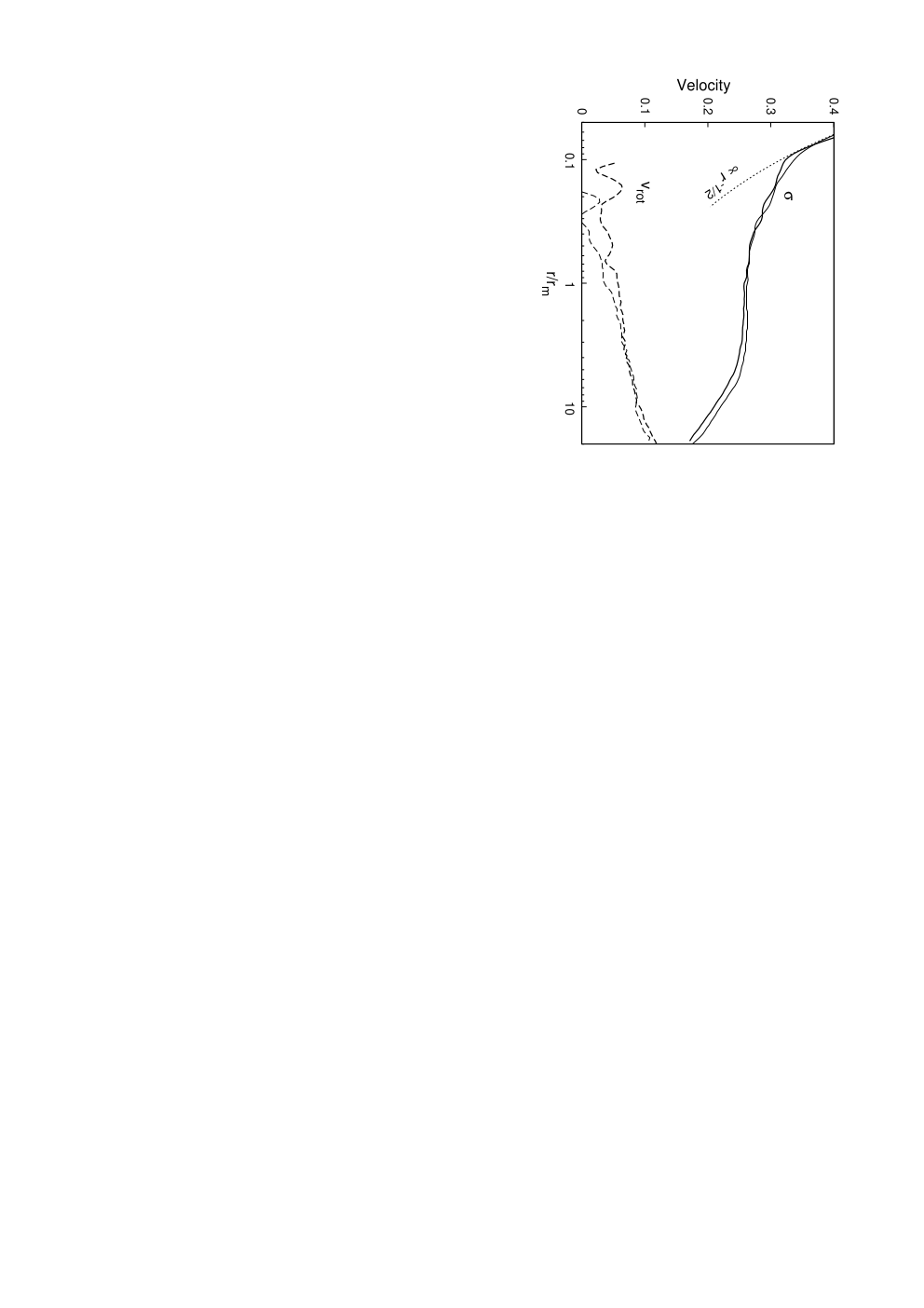
Somewhat larger changes in nuclear structure and kinematics would result from the dissipationaless (gas-free) merger of two galaxies containing comparably-massive SBHs [72]. This is a likely model for the origin of the cores that are observed at the centers of galaxies with [73]. Orbital motion of the two galaxies would imprint rotation on the stars in the merged galaxy, but the binary SBH also displaces a mass in stars of order its own mass via the gravitational slingshot [74]; the net rotation of the stars left behind depends in a complicated way on this process. Figure 19 shows results extracted from perhaps the highest-resolution study to date of this interaction [71]. The figure shows the velocity dispersion and rotation velocity profiles of the merged galaxy at the time when two SBHs coalesce. Despite limited statistics at small radii, it is clear that such merger products may have a noticeable degree of rotation well within the radius of influence, corresponding roughly to .
Both infall of gas clouds and inspiral of massive compact objects could occur episodically. In the case of spiral galaxies, the example of the Milky Way with its young stellar disks suggests that accretion events might occur roughly once per Gyr [75]. In the case of massive galaxies, which tend to be gas-poor, large-scale simulations of dark-matter clustering suggest that the mean time between galaxy mergers varies from Gyr at a redshift to Gyr at with a weak dependence on galaxy (i.e. dark halo) mass [76]. Assuming that all or most galaxies contain nuclear SBHs, this would also be roughly the time between insertion of secondary SBHs into the nucleus [3]. These times are comparable with the time scales for spin precession derived here (e.g. Figure 12), suggesting that the evolution of SBH spins due to frame dragging may also be episodic in nature.
Both sorts of infall event are likely to occur from essentially random directions, so that the increase over time of the net rotation of the nucleus will have the form of a random walk. Futhermore, both sorts of event can change the magnitude of : if accretion of the gas by the SBH occurs [61]; or if the inspiralling body coalesces with the SBH [77].
VI.3 Comparison with accretion disk torquing
Interaction of a spinning SBH with a misaligned, gaseous accretion disk is driven by the same frame-dragging torques modelled here. The accretion disk problem has been extensively studied [2, 78, 79, 80, 5, 81], in part because the radio jets that power the classic, double radio sources are believed to be launched perpendicularly to the inner accretion disk. Both the long-term ( yr) stability of jet directions in some active galaxies, as well as the evidence for jet precession in others, is probably linked in fundamental ways to SBH - accretion disk interactions.
Here we sketch the points of similarity and difference between spin evolution driven by a misaligned accretion disk and by a rotating stellar nucleus. We emphasize that the latter case is generic – SBHs appear always to be embedded in stellar nuclei – while nuclear activity, hence accretion disks, exist in only a small subpopulation of galaxies. The fact that accretion disk torques have received essentially all the attention until now is probably a consequence of the easy observability of the jets.
Given an assumed structure for the disk (surface density and inclination as functions of radius), the instantaneous evolution equation for is essentially Eq. (8), after setting orbital eccentricities in that equation to zero and identifying with the angular momentum of a discrete element of gas. Such models typically assume a disk that is thin and initially planar. Differential precession then ensues near the SBH; at radii – defined, as in Eq. (27), as the radius containing an angular momentum equal to – the gas precession time is short compared with that of the SBH.
The value of can be computed given a model for the disk surface density. For instance, the steady-state disk models referred to above [60] imply [81]
| (102) | |||||
where , and are defined as in Eq. (96). In active galaxies, all quantities in parentheses aside from the factor containing are of order unity and so pc. This is somewhat smaller than the value of as plotted in Figure 2, at least in massive galaxies; in other words: accretion disks, when present, are likely to dominate the angular momentum distribution near the SBH, justifying the neglect of stellar torques in these galaxies. In smaller galaxies, Figure 2 suggests that .
Differential precession causes gas near the SBH to attain a mean that is aligned with , as in the stellar case, but gaseous viscosity also ensures that the gas returns to a thin disk, coincident with the SBH equatorial plane (the “Bardeen-Petterson effect” [2]). This thin, aligned disk extends outward, not to (where the Lense-Thirring time is likely to be very long anyway), but rather to the smaller radius , the radius at which the disk plane transitions to its large-radius orientation. The warp radius is determined by the condition that the time scale for angular momentum diffusion through the disk is equal to the Lense-Thirring precession time:
| (103) |
Here is the kinematic viscosity, which also determines the accretion rate. The value of is strongly model-dependent and still rather uncertain; early estimates (e.g. [2, 79]) set , but more recent estimates (e.g. [5, 82]) find .
Once alignment of the gas inside has occurred, precession of the SBH is driven by gas at . An expression that is often given for the steady-state SBH precession frequency (e.g. [79, 5]) is
| (104) |
where is the angular momentum of disk gas inside . Uncertainties about the value of translate via this expression into uncertainties about the precession rate. Equation (104) is similar to Eq. (14) for the mutual precession of a SBH and a ring of matter, especially when it is recognized that in the accretion-disk case. This is at first sight surprising, since Eq. (104) appears to relate the precession of the SBH to the angular momentum of gas all of which, by assumption, is fully aligned with the SBH! The justification (e.g. [79]) consists of noting that is a steeply falling function of radius, hence only matter near the warp is relevant. But this argument underscores the very approximate nature of Eq. (104).
The warp radius plays approximately the same role as the radius in the stellar case, Eq. (53). The SBH precession frequency, Eq. (104) in the gaseous case, becomes Eq. (80) in the stellar case. In the stellar case, (Figure 2), just as (at least if the most recent estimates of are correct).
The continued deposition of matter from a fixed outer plane must ultimately align with the outer . In many models [80, 5, 83], the time scale for this alignment is similar to the warp-driven precession time of the SBH, i.e. the inverse of Eq. (104). Typical values quoted for lie in the range years and it has been argued that this alignment is responsible for the long-term ( yr) stability of jet directions in many active galaxies. Interestingly, we found that complete alignment was possible also in the stellar-dynamical case (Figure 4); differential precession is sufficient to achieve this, even in the absence of viscosity. However we argued that a more generic outcome in the stellar case is steady precession of the SBH, particularly when stellar interactions are allowed.
The evolution of due to the combined influence of a misaligned accretion disk and stars is beyond the scope of this paper, but we include a few speculative remarks 44 4 Torquing or heating of an accretion disk by stars has been considered by a number of authors [91, 92, 93]; the latter authors also considered reaction of SBH spin to changes in the accretion disk. Feeding of active galaxies is probably episodic [84, 85]. When much, but not all, of the infalling gas has been consumed, there may come a time when the precession rates due to gas and stellar torquing are comparable. If the SBH is still active at this time, accretion-disk-related jets should begin to precess roughly in the manner discussed here, even if the SBH had previously reached a steady-state alignment with the gas. Prolonged, steady precession of radio sources might be explained in this way [86, 87]. After the gas has been fully consumed, the SBH spin can continue to evolve in response to the stars. If the gas has been accreted all the way to the event horizon, both the magnitude and direction of will have been changed by the gas.
VI.4 Slowly-rotating nuclei
Even in a nucleus with negligible net rotation, there will still be a nonzero torque on the SBH due to imperfect cancellation of the from the finite number of stars. This is obvious, for instance, from Figure 8; the components of perpendicular to the mean rotation axis of the cluster are zero on average but fluctuate as orbits change their due to encounters. Eq. (73) is an estimate of the size of those fluctuations and can equally well be interpreted as the expected value of in a nonrotating, isotropic cluster with known .
It is interesting to ask how large the steady rotation of a nucleus needs to be if the net torque exerted on the SBH is to exceed this (fluctuating) value. We estimate the torque in a nonrotating nucleus by setting in Eq. (73); in other words, we conservatively ignore the torque from stars within the sphere of rotational influence given that they may have differentially precessed about . The result is
| (105) |
where in low-mass galaxies and in high-mass galaxies. Comparing to as given by Eq. (80), we find for the critical degree of rotation
| (106) | |||||
For instance, in a low-mass galaxy with ,
| (107) |
For this value of , the instantaneous time over which changes is
| (108) |
We emphasize that this is not a precessional period since, by assumption, finite- effects dominate and the axis about which is precessing will itself change, in a time of order .

When observing changes in over very short time scales, e.g. human lifetimes, there will also be a time-dependent contribution due to the motion of stars along their (unperturbed) orbits. This contribution has been ignored up till now due to the orbit-averaging of Eqs. (8)-(9).
Figure 20 illustrates the complexity of the evolution of in the case that all the torque on the SBH is due to these finite- effects. The figure is based on a direct -body integration of a cluster of “stars,” of mass each, around a SBH of mass and . Additional details about the initial models are given in Merritt et al. (2011) [37]. Over the Myr time span of the integration, the SBH spin axis wobbles by about one degree.
VI.5 Experimental determination of black hole spins
Several authors [58, 88, 89] have suggested that it may be possible to infer the magnitude and direction of SBH spins from the precession of the angular momentum vectors of individual stars. Only stars with semimajor axes are suitable for this purpose, otherwise the changes of due to collisional effects will supersede changes due to frame dragging [32, 90]. Since for most galaxies (Figure 2), this also means that the Lense-Thirring precession times for these stars are much shorter than SBH spin precession times, or .
Assuming that precesses steadily about the (fixed) axis , it is convenient to consider the evolution of in the reference frame which rotates with the precession frequency about the axis of SBH precession, so that is stationary. In this rotating frame, the equation of motion for the orbital angular momenta (9a) reads
| (109) |
where is the angular momentum in the rotating frame. In other words: the Lense-Thirring precession is occuring about an axis that does not coincide with the instantaneous direction of . However, the first derivative of in the inertial frame coincides with the value obtained without taking into account SBH precession, since it is determined by the instantaneous value and direction of . It is only for the second derivative of that the difference starts to matter. Given that because we are considering stars that themselves precess much faster than the SBH, it seems unlikely that these effects may be detectable in the near future.
In a nucleus that is sufficiently old, differential precession of stars with will have caused their angular momentum vectors to distribute themselves uniformly about , as shown above in several numerical examples. This suggests a way of measuring the instantaneous direction of via the mean direction of the within . In the Galactic center, pc, and there are as yet no stars with determined orbits in this region. However orbital periods for stars with mpc are about one year, and it is possible that determination of the orbital elements of a few such stars might be feasible over a shorter time interval than is required for measuring changes in the due to frame dragging.
VII Conclusions
1. In a galactic nucleus containing a spinning supermassive black hole (SBH), frame dragging results in mutual torques between the stellar orbits and the SBH. The result is precession of both the SBH spin, , and the angular momentum vectors, , of the individual stellar orbits, with conserved. For stars at a single distance from the SBH, the controlling parameter is the ratio between and . If , stellar orbits precess about the nearly fixed with the Lense-Thirring period; while if , precesses about the nearly fixed with a period that is shorter by a factor . The inner parsec of the Milky Way is known to contain stellar subsystems having .
2. Ignoring interactions between the stars, solutions of the coupled equations for and in spherical nuclei reveal two evolutionary modes in the case that : continued precession of about ; or damped precession, in which and come into nearly complete alignment after one precessional period of the SBH. Even in the first mode, differential precession of orbits near the SBH causes their net angular momentum to align with , reducing the torque that they exert on the SBH. Subsequent precession of the SBH is driven by torques from stars at , where is the radius enclosing a net angular momentum equal to .
3. Newtonian interactions between stars can change their orbital angular momenta in a time shorter than Lense-Thirring precessional times. We define the “radius of rotational influence,” , around a Kerr SBH as the radius inside of which torques due to frame dragging act more quickly than torques from the other stars. Typical values for this radius are parsecs in dense nuclei like that of the Milky Way, increasing to parsecs in nuclei containing the most massive SBHs. The angular momentum associated with stars in this “collisionless” region near the SBH is likely to be much smaller than in nuclei of the smallest galaxies but may be comparable to in massive galaxies.
4. Interaction between stars at leaves the total angular momentum of these stars unchanged, but results in random fluctuations of the individual and hence in the torque which they exert on the SBH. We develop a stochastic model, based on the Ornstein-Uhlenbeck equation, for the torque exerted by these stars and verify it by comparison with high-accuracy -body simulations. We argue that can be approximated as the sum of two terms: deterministic torques exerted by stars inside , whose angular momenta evolve solely in response to frame-dragging; and a stochastically-fluctuating torque due to stars outside .
5. Examples of stochastic evolution of are presented for various nuclear models. Typical evolution consists of sustained precession, with periods that are highly dependent on nuclear parameters, but which are expected to increase with increasing : likely periods are yr for low-mass SBHs in dense nuclei, yr for SBH with masses , and yr for the most massive SBHs.
Acknowledgements.
DM was supported in part by the National Science Foundation under grant no. 08-21141 and by the National Aeronautics and Space Administration under grant no. NNX-07AH15G. S. Trippe kindly provided data used in Figure 18 and A. Gualandris assisted with Figure 19. We thank T. Alexander, E. Blackman, P. Kharb, A. King, A Robinson, and C. Will for helpful discussions.Appendix A Time scale for change in orbital eccentricity
Here we present approximate expressions [16] for the time scales associated with changes in orbital eccentricity due to resonant relaxation [33] and evaluate them for the power-law density model used in the text.
Define the “apsidal coherence time” as the shorter of the two precession times and defined in §V, each evaluated at typical values of ; say, . Comparison of Eqs. (41) and (50) shows that where is the number of stars at : apsidal precession due to the spherically-distributed mass acts more rapidly than torques at changing orbital orientations. For elapsed times short compared with , the torque due to all the local stars is therefore nearly constant, and the angular momentum of a typical star responds by changing approximately linearly with time. In this “coherent resonant relaxation” regime, all the components of , i.e. both the orientation angles and the eccentricity , change with characteristic time given by
| (110) |
This is the same expression as Eq. (50) for , reflecting the fact that in the coherent regime, both the direction and the magnitude of change on roughly the same time scale.
For time intervals longer than , the direction of the net field-star torque changes, and evolution of the in response to the torques is better described as a random walk. The time scale associated with this “incoherent resonant relaxation” is
| (111) |
where is the angular momentum of a circular orbit of semimajor axis , and is the change in during . Setting (i.e. ), this becomes
| (112) |
with a constant of order unity, while if (),
| (113) |
with again of order unity. Eqs. (112) and (113) are the appropriate time scales to associate with changes in orbital eccentricity in the incoherent regime.
In the case of 2d resonant relaxation, the relevant coherence time is that associated with changes of the orbital planes, i.e. . Since in this case, Eq. (111) implies that the coherent and incoherent relaxation times are approximately the same: no new time scale arises in the incoherent regime for 2d resonant relaxation.
Comparing the incoherent relaxation times associated with changes in the orientation and magnitude of , respectively, we find
| (114a) | |||||
| (114b) | |||||
The first of these ratios is manifestly smaller than unity at all radii. The second is only relevant at , i.e. for
| (115) |
which implies
| (116) |
again less than unity. On the basis of these inequalities, it is reasonable to equate the correlation time associated with fluctuations in with the shortest of the time scales, , as was done in §V.2.
References
- [1] J. Lense and H. Thirring, Physikalische Zeitschrift 19, 156 (1918).
- [2] J. M. Bardeen and J. A. Petterson, Astrophys. J. Letts. 195, L65 (1975).
- [3] M. C. Begelman, R. D. Blandford, and M. J. Rees, Nature 287, 307 (1980).
- [4] N. Roos, Astrophys. J. 334, 95 (1988).
- [5] P. Natarajan and J. E. Pringle, Astrophys. J. Letts. 506, L97 (1998), eprint arXiv:astro-ph/9808187.
- [6] L. E. Kidder, Phys. Rev. D 52, 821 (1995).
- [7] T. Paumard, R. Genzel, F. Martins, S. Nayakshin, A. M. Beloborodov, Y. Levin, S. Trippe, F. Eisenhauer, T. Ott, S. Gillessen, et al., Astrophys. J. 643, 1011 (2006), eprint arXiv:astro-ph/0601268.
- [8] J. R. Lu, A. M. Ghez, S. D. Hornstein, M. R. Morris, E. E. Becklin, and K. Matthews, Astrophys. J. 690, 1463 (2009), eprint 0808.3818.
- [9] H. Bartko, F. Martins, S. Trippe, T. K. Fritz, R. Genzel, T. Ott, F. Eisenhauer, S. Gillessen, T. Paumard, T. Alexander, et al., Astrophys. J. 708, 834 (2010), eprint 0908.2177.
- [10] S. Gillessen, F. Eisenhauer, S. Trippe, T. Alexander, R. Genzel, F. Martins, and T. Ott, Astrophys. J. 692, 1075 (2009), eprint 0810.4674.
- [11] R. Schödel, A. Eckart, T. Alexander, D. Merritt, R. Genzel, A. Sternberg, L. Meyer, F. Kul, J. Moultaka, T. Ott, et al., Astron. Astrophys. 469, 125 (2007), eprint arXiv:astro-ph/0703178.
- [12] R. Schödel, D. Merritt, and A. Eckart, Astron. Astrophys. 502, 91 (2009), eprint 0902.3892.
- [13] D. Merritt, Astrophys. J. 718, 739 (2010), eprint 0909.1318.
- [14] R. Schödel, in Astronomical Society of the Pacific Conference Series, edited by M. R. Morris, Q. D. Wang, & F. Yuan (2011), vol. 439 of Astronomical Society of the Pacific Conference Series, p. 222, eprint 1001.4238.
- [15] S. Trippe, S. Gillessen, O. E. Gerhard, H. Bartko, T. K. Fritz, H. L. Maness, F. Eisenhauer, F. Martins, T. Ott, K. Dodds-Eden, et al., Astron. Astrophys. 492, 419 (2008), eprint 0810.1040.
- [16] D. Merritt, Dynamics and Evolution of Galactic Nuclei (Princeton, NJ, Princeton University Press, 665 pp., 2013).
- [17] A. Einstein, Ann. Math. 40, 922 (1939).
- [18] A. W. Graham, ArXiv e-prints (2011), eprint 1108.0997.
- [19] D. Merritt, J. D. Schnittman, and S. Komossa, Astrophys. J. 699, 1690 (2009), eprint 0809.5046.
- [20] K. Gebhardt, D. Richstone, E. A. Ajhar, T. R. Lauer, Y. Byun, J. Kormendy, A. Dressler, S. M. Faber, C. Grillmair, and S. Tremaine, Astron. J. 112, 105 (1996).
- [21] P. Côté, L. Ferrarese, A. Jordán, J. P. Blakeslee, C.-W. Chen, L. Infante, D. Merritt, S. Mei, E. W. Peng, J. L. Tonry, et al., Astrophys. J. 671, 1456 (2007), eprint 0711.1358.
- [22] S. Oh, S. S. Kim, and D. F. Figer, Journal of Korean Astronomical Society 42, 17 (2009), eprint 0906.0765.
- [23] D. Merritt, Astrophys. J. 694, 959 (2009), eprint 0802.3186.
- [24] S. E. Woosley, A. Heger, and T. A. Weaver, Reviews of Modern Physics 74, 1015 (2002).
- [25] J. N. Bahcall and R. A. Wolf, Astrophys. J. 209, 214 (1976).
- [26] J. N. Bahcall and R. A. Wolf, Astrophys. J. 216, 883 (1977).
- [27] C. Hopman and T. Alexander, Astrophys. J. Letts. 645, L133 (2006), eprint arXiv:astro-ph/0603324.
- [28] M. Freitag, P. Amaro-Seoane, and V. Kalogera, ArXiv Astrophysics e-prints (2006), eprint arXiv:astro-ph/0603280.
- [29] R. M. Buchholz, R. Schödel, and A. Eckart, Astron. Astrophys. 499, 483 (2009), eprint 0903.2135.
- [30] T. Do, A. M. Ghez, M. R. Morris, J. R. Lu, K. Matthews, S. Yelda, and J. Larkin, Astrophys. J. 703, 1323 (2009), eprint 0908.0311.
- [31] R. W. Brankin, I. Gladwell, and L. F. Shampine, Tech. Rep., Southern Methodist University, Dallas (1991).
- [32] D. Merritt, T. Alexander, S. Mikkola, and C. M. Will, Physical Review D 81, 062002 (2010), eprint 0911.4718.
- [33] K. P. Rauch and S. Tremaine, New Astron. 1, 149 (1996), eprint arXiv:astro-ph/9603018.
- [34] D. Merritt and E. Vasiliev, The Astrophysical Journal 726, 61 (2011), eprint 1005.0040.
- [35] H. B. Perets, C. Hopman, and T. Alexander, Astrophys. J. 656, 709 (2007), eprint arXiv:astro-ph/0606443.
- [36] E. Eilon, G. Kupi, and T. Alexander, Astrophys. J. 698, 641 (2009), eprint 0807.1430.
- [37] D. Merritt, T. Alexander, S. Mikkola, and C. M. Will, Physical Review D 84, 044024 (2011), eprint 1102.3180.
- [38] A.-M. Madigan, C. Hopman, and Y. Levin, Astrophys. J. 738, 99 (2011), eprint 1010.1535.
- [39] S. Mikkola and D. Merritt, Mon. Not. R. Astron. Soc. 372, 219 (2006), eprint arXiv:astro-ph/0605054.
- [40] S. Mikkola and D. Merritt, Astron. J. 135, 2398 (2008), eprint 0709.3367.
- [41] T. Damour and N. Deruelle, Annales de l’I.H.P. Physique thorique 43, 107 (1985).
- [42] N. G. van Kampen, Stochastic Processes in Physics and Chemistry (Elsevier Science, Amsterdam, 1992).
- [43] G. E. Uhlenbeck and L. S. Ornstein, Physical Review 36, 823 (1930).
- [44] D. T. Gillespie, Phys. Rev. E 54, 2084 (1996).
- [45] F. Reif, Fundamentals of Statistical and Thermal Physics (Waveland Press, 1965).
- [46] G. Worthey, Astrophys. J. Suppl. 95, 107 (1994).
- [47] A. Marconi and L. K. Hunt, Astrophys. J. Letts. 589, L21 (2003), eprint arXiv:astro-ph/0304274.
- [48] M. T. McGinn, K. Sellgren, E. E. Becklin, and D. N. B. Hall, Astrophys. J. 338, 824 (1989).
- [49] A. W. McConnachie, M. J. Irwin, A. M. N. Ferguson, R. A. Ibata, G. F. Lewis, and N. Tanvir, Mon. Not. R. Astron. Soc. 356, 979 (2005), eprint arXiv:astro-ph/0410489.
- [50] M. Valluri, L. Ferrarese, D. Merritt, and C. L. Joseph, Astrophys. J. 628, 137 (2005).
- [51] C. L. Joseph, D. Merritt, R. Olling, M. Valluri, R. Bender, G. Bower, A. Danks, T. Gull, J. Hutchings, M. E. Kaiser, et al., Astrophys. J. 550, 668 (2001), eprint arXiv:astro-ph/0005530.
- [52] E. K. Verolme, M. Cappellari, Y. Copin, R. P. van der Marel, R. Bacon, M. Bureau, R. L. Davies, B. M. Miller, and P. T. de Zeeuw, Mon. Not. R. Astron. Soc. 335, 517 (2002).
- [53] E. Emsellem, H. Dejonghe, and R. Bacon, Mon. Not. R. Astron. Soc. 303, 495 (1999).
- [54] Y. Copin, N. Cretton, and E. Emsellem, Astron. Astrophys. 415, 889 (2004), eprint arXiv:astro-ph/0311387.
- [55] K. L. Shapiro, M. Cappellari, T. de Zeeuw, R. M. McDermid, K. Gebhardt, R. C. E. van den Bosch, and T. S. Statler, Mon. Not. R. Astron. Soc. 370, 559 (2006), eprint arXiv:astro-ph/0605479.
- [56] N. Cretton and F. C. van den Bosch, Astrophys. J. 514, 704 (1999), eprint arXiv:astro-ph/9811180.
- [57] C. Siopis, K. Gebhardt, T. R. Lauer, J. Kormendy, J. Pinkney, D. Richstone, S. M. Faber, S. Tremaine, M. C. Aller, R. Bender, et al., Astrophys. J. 693, 946 (2009), eprint 0808.4001.
- [58] Y. Levin and A. M. Beloborodov, Astrophys. J. Letts. 590, L33 (2003), eprint arXiv:astro-ph/0303436.
- [59] S. Nayakshin and J. Cuadra, Astron. Astrophys. 437, 437 (2005), eprint arXiv:astro-ph/0409541.
- [60] S. Collin-Souffrin and A. M. Dumont, Astron. Astrophys. 229, 292 (1990).
- [61] A. R. King and J. E. Pringle, Mon. Not. R. Astron. Soc. 377, L25 (2007), eprint arXiv:astro-ph/0701679.
- [62] N. I. Shakura and R. A. Sunyaev, Astron. Astrophys. 24, 337 (1973).
- [63] S. Nayakshin, W. Dehnen, J. Cuadra, and R. Genzel, Mon. Not. R. Astron. Soc. 366, 1410 (2006), eprint arXiv:astro-ph/0511830.
- [64] J. Cuadra, S. Nayakshin, and R. Sunyaev, Astron. Astrophys. 411, 405 (2003), eprint arXiv:astro-ph/0304533.
- [65] S. Nayakshin, J. Cuadra, and R. Sunyaev, Astron. Astrophys. 413, 173 (2004), eprint arXiv:astro-ph/0304126.
- [66] G. C. Bower, M. C. H. Wright, H. Falcke, and D. C. Backer, Astrophys. J. 588, 331 (2003), eprint arXiv:astro-ph/0302227.
- [67] I. A. Bonnell and W. K. M. Rice, Science 321, 1060 (2008), eprint 0810.2723.
- [68] A. Hobbs and S. Nayakshin, Mon. Not. R. Astron. Soc. 394, 191 (2009), eprint 0809.3752.
- [69] C. Alig, A. Burkert, P. H. Johansson, and M. Schartmann, Mon. Not. R. Astron. Soc. 412, 469 (2011), eprint 0908.1100.
- [70] M. Mapelli, T. Hayfield, L. Mayer, and J. Wadsley, Astrophys. J. 749, 168 (2012), eprint 1202.0555.
- [71] A. Gualandris and D. Merritt, Astrophys. J. 744, 74 (2012), eprint 1107.4095.
- [72] M. Milosavljević and D. Merritt, Astrophys. J. 563, 34 (2001).
- [73] D. Merritt, Astrophys. J. 648, 976 (2006), eprint arXiv:astro-ph/0603439.
- [74] S. Mikkola and M. J. Valtonen, Mon. Not. R. Astron. Soc. 259, 115 (1992).
- [75] T. Alexander, Physics Reports 419, 65 (2005).
- [76] O. Fakhouri, C.-P. Ma, and M. Boylan-Kolchin, Mon. Not. R. Astron. Soc. 406, 2267 (2010), eprint 1001.2304.
- [77] D. Merritt and R. D. Ekers, Science 297, 1310 (2002).
- [78] M. J. Rees, Nature 275, 516 (1978).
- [79] C. L. Sarazin, M. C. Begelman, and S. P. Hatchett, Astrophys. J. Letts. 238, L129 (1980).
- [80] P. A. G. Scheuer and R. Feiler, Mon. Not. R. Astron. Soc. 282, 291 (1996).
- [81] A. R. King, S. H. Lubow, G. I. Ogilvie, and J. E. Pringle, Mon. Not. R. Astron. Soc. 363, 49 (2005), eprint arXiv:astro-ph/0507098.
- [82] R. G. Martin, J. E. Pringle, and C. A. Tout, Mon. Not. R. Astron. Soc. 381, 1617 (2007), eprint 0708.2034.
- [83] G. Lodato and J. E. Pringle, Mon. Not. R. Astron. Soc. 368, 1196 (2006), eprint arXiv:astro-ph/0602306.
- [84] A. P. Schoenmakers, A. G. de Bruyn, H. J. A. Röttgering, H. van der Laan, and C. R. Kaiser, Mon. Not. R. Astron. Soc. 315, 371 (2000), eprint arXiv:astro-ph/9912141.
- [85] P. Kharb, C. P. O’Dea, S. A. Baum, E. J. M. Colbert, and C. Xu, Astrophys. J. 652, 177 (2006), eprint arXiv:astro-ph/0607603.
- [86] A. C. Gower, P. C. Gregory, W. G. Unruh, and J. B. Hutchings, Astrophys. J. 262, 478 (1982).
- [87] J.-F. Lu and B.-Y. Zhou, Astrophys. J. Letts. 635, L17 (2005), eprint arXiv:astro-ph/0511212.
- [88] C. M. Will, Astrophys. J. Letts. 674, L25 (2008), eprint 0711.1677.
- [89] F. Eisenhauer, G. Perrin, W. Brandner, C. Straubmeier, K. Perraut, A. Amorim, M. Schöller, S. Gillessen, P. Kervella, M. Benisty, et al., The Messenger 143, 16 (2011).
- [90] L. Sadeghian and C. M. Will, Classical and Quantum Gravity 28, 225029 (2011), eprint 1106.5056.
- [91] J. P. Ostriker, Astrophys. J. 273, 99 (1983).
- [92] E. Y. Vilkoviskij, Pis ma Astronomicheskii Zhurnal 9, 405 (1983).
- [93] M. Bregman and T. Alexander, Astrophys. J. 748, 63 (2012), eprint 1109.5384.