Extended phase space thermodynamics for charged and rotating black holes and Born–Infeld vacuum polarization

The solution for a spherical charged AdS black hole in $d>3$ spacetime dimensions reads

	$\displaystyle ds^{2}$	$\displaystyle=$	$\displaystyle-fdt^{2}+\frac{dr^{2}}{f}+r^{2}d\Omega_{d-2}^{2}\,,$
	$\displaystyle F$	$\displaystyle=$	$\displaystyle dA\,,\quad A=-\sqrt{\frac{d-2}{2(d-3)}}\frac{q}{r^{d-3}}dt\,.$		(1)

Here, $d\Omega_{d}^{2}$ stands for the standard element on $S^{d}$ and function $f$ is given by

$$f=1-\frac{m}{r^{d-3}}+\frac{q^{2}}{r^{2(d-3)}}+\frac{r^{2}}{l^{2}}\,.$$

(2)

Parameters $m$ and $q$ are related to the ADM mass $M$ (in our set up associated with the enthalpy of the system as we shall see) and the black hole charge $Q$ as [2]

	$\displaystyle M$	$\displaystyle=$	$\displaystyle\frac{d-2}{16\pi}\omega_{d-2}m\,,$
	$\displaystyle Q$	$\displaystyle=$	$\displaystyle\frac{\sqrt{2(d-2)(d-3)}}{8\pi}\,\omega_{d-2}\,q\,,$		(3)

with $\omega_{d}$ being the volume of the unit $d$-sphere,

$$\omega_{d}=\frac{2\pi^{\frac{d+1}{2}}}{\Gamma\left(\frac{d+1}{2}\right)}\,.$$

(4)

The metric and the gauge field (1) solve the Einstein–Maxwell equations following from the bulk action

$$I_{EM}=-\frac{1}{16\pi}\int_{M}d^{d}x\sqrt{-g}\Bigl(R-F^{2}+\frac{(d-1)(d-2)}{l^{2}}\Bigr)\,.$$

(5)

In our considerations we interpret the cosmological constant $\Lambda=-\frac{(d-1)(d-2)}{2l^{2}}$ as a thermodynamic pressure $P$,

$$P=-\frac{1}{8\pi}\Lambda=\frac{(d-1)(d-2)}{16\pi l^{2}}\,.$$

(6)

The corresponding conjugate quantity, the thermodynamic volume, is given by [9]

$$V=\frac{\omega_{d-2}{r_{+}}^{d-1}}{d-1}\,.$$

(7)

The black hole temperature reads

$$T=\frac{f^{\prime}(r_{+})}{4\pi}=\frac{d-3}{4\pi r_{+}}\Bigl(1-\frac{q^{2}}{r_{+}^{2(d-3)}}+\frac{d-1}{d-3}\frac{r_{+}^{2}}{l^{2}}\Bigr)\,,$$

(8)

with $r_{+}$ being the position of black hole horizon, determined from $f(r_{+})=0$. The black hole entropy $S$ and the electric potential $\Phi$ (measured at infinity with respect to the horizon) are

	$\displaystyle S$	$\displaystyle=$	$\displaystyle\frac{A_{d-2}}{4},\quad A_{d-2}=\omega_{d-2}r_{+}^{d-2}\,,$		(9)
	$\displaystyle\Phi$	$\displaystyle=$	$\displaystyle\sqrt{\frac{d-2}{2(d-3)}}\frac{q}{r_{+}^{d-3}}\,.$		(10)

All these quantities satisfy the following Smarr formula:

$$M=\frac{d-2}{d-3}TS+\Phi Q-\frac{2}{d-3}VP\,,$$

(11)

as well as the (extended phase-space) 1st law of black hole thermodynamics

$$dM=TdS+\Phi dQ+VdP\,.$$

(12)

These two are related by a dimensional (scaling) argument; see, e.g., [5].

In the canonical (fixed charge $Q$) ensemble¹¹ 1 For thermodynamics in the grand canonical (fixed potential $\Phi$) ensemble see [11]. a first order phase transition in the $(T,Q)$-plane, reminiscent of the liquid–gas phase transition of the Van der Waals fluid was noted quite some time ago in the context of a fixed cosmological constant [2, 3]. The properties of the corresponding critical point have been elaborated, for example, in [12]. More recently, however, it has been pointed out [4] that at least in 4D the corresponding critical behaviour has a more natural interpretation in the extended phase space (where the cosmological constant is treated as a thermodynamic pressure), giving the phase transition in the $(P,T)$-plane, making the similarity with the Van der Waals fluid complete. In what follows we shall study this situation in the higher-dimensional case.

The critical behaviour of a system is captured by its partition function: namely the thermodynamic potential, associated with the Euclidean action, calculated at fixed $Q$, fixed $P$ and fixed $T$ is the Gibbs free energy. Using the counterterm method (canceling the AdS divergences) [13, 14] and the following boundary term (characteristic for the canonical ensemble [15]):

$$I_{b}=-\frac{1}{4\pi}\int d^{d-1}x\sqrt{h}F^{ab}n_{a}A_{b}\,,$$

(13)

the Gibbs free energy $G=M-TS$ reads [2]

$$G=G(P,T)=\!\frac{{\omega}_{d-2}}{16\pi}\biggl(\!r_{+}^{d-3}-\frac{16\pi Pr_{+}^{d-1}}{(d\!-\!1)(d\!-\!2)}+\frac{(2d\!-\!5)q^{2}}{r_{+}^{d-3}}\biggl).\ \$$

(14)

Here, $r_{+}$ is understood to be a function of the black hole temperature $T$ and pressure $P$ via equations (6) and (8); upon employing (7) we obtain

$$P=\frac{T(d-2)}{4r_{+}}-\frac{(d-3)(d-2)}{16\pi r_{+}^{2}}+\frac{q^{2}(d-3)(d-2)}{16\pi r_{+}^{2(d-2)}}\,.$$

(15)

The behaviour of $G$ for dimensions $d=4$ and $d=10$ is depicted in Figs. 1 and 2, respectively; we see from these figures the characteristic 1st-order phase transition behaviour.

To make contact with the Van der Waals fluid in $d$ dimensions (see App. B), note that in any dimension $d$ we have $l_{P}^{d-2}=G_{d}\hbar/c^{3}$, where pressure has units of energy per volume. We thus identify the following relations between our ‘geometric quantities’ $P$ and $T$ and the physical pressure and temperature:

$$[\mbox{Press}]=\frac{\hbar c}{l_{p}^{d-2}}[P]\,,\quad[\mbox{Temp}]=\frac{\hbar c}{k}[T]\,.$$

(16)

Therefore

	Press	$\displaystyle=$	$\displaystyle\frac{\hbar c}{l_{p}^{d-2}}P=\frac{\hbar c}{l_{p}^{d-2}}\frac{(d-2)T}{4r_{+}}+\dots$		(17)
		$\displaystyle=$	$\displaystyle\frac{k\mbox{Temp}(d-2)}{4l_{p}^{d-2}r_{+}}+\dots$

Comparing with the Van der Waals equation, (139), we conclude that we should identify the specific volume $v$ of the fluid with the horizon radius of the black hole as

$$v=\frac{4r_{+}l_{P}^{d-2}}{d-2}\,.$$

(18)

In geometric units we have

$$r_{+}=\kappa v\,,\quad\kappa=\frac{d-2}{4}\,,$$

(19)

and the equation of state reads

$$P=\frac{T}{v}-\frac{(d-3)}{\pi(d-2)v^{2}}+\frac{q^{2}(d-3)}{4\pi v^{2(d-2)}\kappa^{2d-5}}\,.$$

(20)

The associated $P-v$ diagram²² 2 Throughout our paper we display $P-v$ diagrams, with $v$ being the specific volume of the corresponding fluid, rather than $P-V$ diagrams, with $V$ being the thermodynamic volume. In $d$ dimensions the two are related via $$V=\frac{\omega_{d-2}}{d-1}\left(\frac{d-2}{4}\right)^{d-1}\!\!v^{d-1}\,.$$ for a 4D black hole is displayed in Fig. 3. Obviously, for $T<T_{c}$ there is a small–large black hole phase transition in the system. This qualitative behaviour persists in higher dimensions—see Fig. 4 for an illustration in $d=10$.

Critical points occur at stationary points of inflection in the $P-v$ diagram, where

$$\frac{\partial P}{\partial v}=0\,,\quad\frac{{\partial}^{2}P}{{\partial}v^{2}}=0\,,$$

(21)

yielding

	$\displaystyle v_{c}$	$\displaystyle=$	$\displaystyle\frac{1}{\kappa}\left[q^{2}(d-2)(2d-5)\right]^{1/[2(d-3)]}\,,$
	$\displaystyle T_{c}$	$\displaystyle=$	$\displaystyle\frac{(d-3)^{2}}{\pi\kappa v_{c}(2d-5)}\,,$
	$\displaystyle P_{c}$	$\displaystyle=$	$\displaystyle\frac{(d-3)^{2}}{16\pi{\kappa}^{2}{v_{c}}^{2}}\,.$		(22)

This gives the following universal (independent of $q$) ratio

$${\rho}_{c}=\frac{P_{c}v_{c}}{T_{c}}=\frac{2d-5}{4d-8}\,.$$

(23)

Note that only in $d=4$ do we recover the ratio $\rho_{c}=3/8$, characteristic for a Van der Waals fluid in any number of spacetime dimensions.

The coexistence line in the $(P,T)$-plane is displayed in Figs. 5-6.

Following the approach taken previously for $d=4$ [4], we shall now calculate the critical exponents characterizing the behaviour of physical quantities in the vicinity of the critical point found in the previous section. The definition of these exponents is for convenience gathered in appendix A.

To calculate the critical exponent $\alpha$ we consider the entropy $S$, (9), as a function of $T$ and $V$. Using (7) we have

$$S=S(T,V)=\omega_{d-2}^{\frac{1}{d-1}}\Bigl[(d-1)V\Bigr]^{\frac{d-2}{d-1}}\,.$$

(24)

Since this is independent of $T$, we have $C_{V}=0$ and hence $\alpha=0$. Defining

$$p=\frac{P}{P_{c}}\,,\quad\nu=\frac{v}{v_{c}}\,,\quad\tau=\frac{T}{T_{c}}\,,$$

(25)

the equation of state (20) translates into the following ‘law of corresponding states’:

$$p=\frac{4(d-2)\tau}{(2d-5)\nu}-\frac{d-2}{(d-3)\nu^{2}}+\frac{1}{(d-3)(2d-5)\nu^{2d-4}}\,.$$

(26)

Although this law has explicit dimensional dependence, we shall show that this does not affect the behaviour of the critical exponents.

Slightly more generally, let us assume (as will be the case for all the examples studied in this paper) that the law of corresponding states takes the form

$$p=\frac{1}{\rho_{c}}\frac{\tau}{\nu}+h(\nu)\,,$$

(27)

where $\rho_{c}$ stand for the critical ratio. Expanding this equation near the critical point

$$\tau=t+1\,,\quad\nu=(\omega+1)^{1/z}\,,$$

(28)

where $z>0$, and using the fact that from the definition of the critical point we have

$$\frac{1}{\rho_{c}}+h(1)=1\,,\quad{\rho_{c}}h^{\prime}(1)=1\,,\quad\rho_{c}h^{\prime\prime}(1)=-2\,,$$

(29)

and so obtain

$$p=1+At-Bt\omega-C\omega^{3}+O(t\omega^{2},\omega^{4})\,,$$

(30)

where

$$A=\frac{1}{\rho_{c}}\,,\quad B=\frac{1}{z\rho_{c}}\,,\quad C=\frac{1}{z^{3}}\left(\frac{1}{\rho_{c}}-\frac{h^{(3)}(1)}{6}\right)\,.$$

(31)

Let us further assume that $C>0$ (again this is for all of the examples). Differentiating the series for a fixed $t<0$ we get

$$dP=-P_{c}(Bt+3C\omega^{2})d\omega\,.$$

(32)

Employing Maxwell’s equal area law, see, e.g., [4], while denoting $\omega_{s}$ and $\omega_{l}$ the ‘volume’ of small and large black holes, we get the following two equations:

	$\displaystyle p$	$\displaystyle=$	$\displaystyle 1+At-Bt\omega_{l}-C\omega_{l}^{3}=1+At-Bt\omega_{s}-C\omega^{3}_{s}\,,$
	$\displaystyle 0$	$\displaystyle=$	$\displaystyle\int_{\omega_{l}}^{\omega_{s}}\omega dP\,.$		(33)

The unique non-trivial solution is

$$\omega_{s}=-\omega_{l}=\sqrt{\frac{-Bt}{C}}\,,$$

(34)

yielding

$$\eta=V_{c}(\omega_{l}-\omega_{s})=2V_{c}\omega_{l}\propto\sqrt{-t}\quad\Rightarrow\quad\beta=\frac{1}{2}\,.$$

(35)

To calculate the exponent $\gamma$, we use again (32), to get

$$\kappa_{T}=-\frac{1}{V}\frac{\partial V}{\partial P}\Big|_{T}\propto\frac{1}{P_{c}}\frac{1}{Bt}\quad\Rightarrow\quad\gamma=1\,.$$

(36)

Finally, the ‘shape of the critical isotherm’ $t=0$ is given by (30), i.e.,

$$p-1=-C\omega^{3}\quad\Rightarrow\quad\delta=3\,.$$

(37)

To conclude, provided that the equation of state takes the form (27), such that the coefficient $C$, given by (31) is non-trivial and positive, we recover the (mean field theory) critical exponents

$$\beta=\frac{1}{2}\,,\quad\gamma=1\,,\quad\delta=3\,.$$

(38)

In particular, for charged AdS black holes in any dimension $d$, the law of corresponding states, (26), takes the form (27). Taking $z=d-1$ (in which case $\omega=\frac{V}{V_{c}}-1$), we obtain the expansion (30) with

$$A=\frac{4d-8}{2d-5}\,,\quad B=\frac{4d-8}{(2d-5)(d-1)}\,,\quad C=\frac{2d-4}{3(d-1)^{3}}$$

(39)

and so the discussion above applies. We conclude that the thermodynamic exponents associated with the charged AdS black hole in any dimension $d>3$ coincide with those of the Van der Waals fluid. We now consider the effects of rotation on these results in the following section.

The charged AdS rotating black hole solution is given by the Kerr-Newman-AdS metric

	$\displaystyle ds^{2}$	$\displaystyle=$	$\displaystyle-\frac{\Delta}{\rho^{2}}\left[dt-\frac{a\sin^{2}\!\theta}{\Xi}d\varphi\right]^{2}+\frac{\rho^{2}}{\Delta}dr^{2}+\frac{\rho^{2}}{S}d\theta^{2}$		(40)
			$\displaystyle+\frac{S\sin^{2}\!\theta}{\rho^{2}}\left[adt-\frac{r^{2}+a^{2}}{\Xi}d\varphi\right]^{2}\,,$

in $d=4$, where

	$\displaystyle\rho^{2}$	$\displaystyle=$	$\displaystyle r^{2}+a^{2}\cos^{2}\!\theta\,,\quad\Xi=1-\frac{a^{2}}{l^{2}}\,,\quad S=1-\frac{a^{2}}{l^{2}}\cos^{2}\!\theta\,,$
	$\displaystyle\Delta$	$\displaystyle=$	$\displaystyle(r^{2}+a^{2})\left(1+\frac{r^{2}}{l^{2}}\right)-2mr+q^{2}\,.$		(41)

The $U(1)$ potential reads

$$A=-\frac{qr}{\rho^{2}}\left(dt-\frac{a\sin^{2}\!\theta}{\Xi}d\varphi\right)\,.$$

(42)

The thermodynamics of charged rotating black holes treating the cosmological constant as independent variable was performed in [16, 9, 7]. In particular, one has the following thermodynamic quantities:

	$\displaystyle S$	$\displaystyle=$	$\displaystyle\frac{\pi(r_{+}^{2}+a^{2})}{\Xi}\,,\quad T=\frac{r_{+}\left(1+\frac{a^{2}}{l^{2}}+3\frac{r_{+}^{2}}{l^{2}}-\frac{a^{2}+q^{2}}{r_{+}^{2}}\right)}{4\pi(r_{+}^{2}+a^{2})}\,,$
	$\displaystyle\Phi$	$\displaystyle=$	$\displaystyle\frac{qr_{+}}{r_{+}^{2}+a^{2}}\,,\quad\Omega_{H}=\frac{a\Xi}{r_{+}^{2}+a^{2}}\,.$		(43)

The mass $M$, the charge $Q$, and the angular momentum $J$ are related to parameters $m$, $q$, and $a$ as follows:

$$M=\frac{m}{\Xi^{2}}\,,\quad Q=\frac{q}{\Xi}\,,\quad J=\frac{am}{\Xi^{2}}\,.$$

(44)

Using the counterterm method [13, 14], the action for the canonical ensemble was calculated in [17, 16] and reads

$$I=\frac{\beta}{4}\left(r_{+}-\frac{r_{+}^{3}}{\Xi l^{2}}+\frac{a^{2}+q^{2}}{r_{+}\Xi}+\frac{2q^{2}r_{+}}{\Xi(r_{+}^{2}+a^{2})}\right)\,.$$

(45)

The corresponding Gibbs free energy reads

$$G=G(P,T,J,Q)=\frac{I}{\beta}+\Omega J\,,$$

(46)

where [16]

$$\Omega=\Omega_{H}-\Omega_{\infty}=\Omega_{H}+\frac{a}{l^{2}}\,.$$

(47)

The thermodynamic volume is [9, 8]

$$V=\frac{2\pi}{3}\frac{(r_{+}^{2}+a^{2})(2r_{+}^{2}l^{2}+a^{2}l^{2}-r_{+}^{2}a^{2})+l^{2}q^{2}a^{2}}{l^{2}\Xi^{2}r_{+}}\,$$

(48)

with the pressure $P=\frac{3}{8\pi}\frac{1}{l^{2}}$ still given by (6). The equation of state is written as

$$T=\frac{r_{+}\left(1+\frac{a^{2}}{l^{2}}+3\frac{r_{+}^{2}}{l^{2}}-\frac{a^{2}+q^{2}}{r_{+}^{2}}\right)}{4\pi(r_{+}^{2}+a^{2})}\,$$

(49)

where we express the parameters $a$ and $q$ in terms of the physical quantities $J$ and $Q$, (44). This gives

	$\displaystyle P$	$\displaystyle=$	$\displaystyle\frac{T}{2r_{+}}-\frac{1}{8\pi r_{+}^{2}}+\frac{Q^{2}}{8\pi r_{+}^{4}}$		(50)
			$\displaystyle+\frac{3(4r_{+}^{4}+8\pi Tr_{+}^{5}-8\pi Tr_{+}^{3}Q^{2}+r_{+}^{2}Q^{2}-2Q^{4})}{8\pi r_{+}^{6}(r_{+}^{2}+2\pi Tr_{+}^{3}+2Q^{2})^{2}}J^{2}$
			$\displaystyle+O(J^{4})\,$

as an expansion in powers of the angular momentum $J$. In what follows we expand all quantities to $O(J^{2})$, neglecting all terms higher order in $J$. We further introduce the following quantity (which we shall see corresponds to the specific volume of the associated Van der Waals fluid)

$$v=2\left(\frac{3V}{4\pi}\right)^{1/3}\!\!\!\!=2r_{+}+\frac{12(8\pi r_{+}^{4}P+3r_{+}^{2}+Q^{2})}{r_{+}(3r_{+}^{2}+8\pi r_{+}^{4}P+3Q^{2})^{2}}J^{2}\,,$$

(51)

and finally obtain the equation of state

	$\displaystyle P$	$\displaystyle=$	$\displaystyle\frac{T}{v}-\frac{1}{2\pi v^{2}}+\frac{2Q^{2}}{\pi v^{4}}+\frac{48J^{2}}{\pi v^{6}}$		(52)
			$\displaystyle-\frac{96Q^{2}(24Q^{2}+5v^{2}+6\pi Tv^{3})J^{2}}{\pi v^{6}(8Q^{2}+v^{2}+\pi Tv^{3})^{2}}\,.\quad$

In what follows we limit ourselves to the case of zero charge $Q=0$, for which (52) becomes [8]

$$P=\frac{T}{v}-\frac{1}{2\pi v^{2}}+\frac{48J^{2}}{\pi v^{6}}\,.$$

(53)

In the same approximation we get the following expression for the Gibbs potential:

$$G=\frac{v}{8}-\frac{\pi Pv^{4}}{12}+\frac{20J^{2}}{v^{3}}\,.$$

(54)

Upon comparing (53) to (20) and (54) to (14) we note the same qualitative behaviour as in the charged case, with fixed $J$ playing the role of fixed $Q$. However the quantitative dependence of $P$ on $v$ is different. We depict the $P-v$ diagram in Fig. 7 and the Gibbs potential in Fig. 8, where the qualitative behaviour is seen to be similar to the non-rotating charged case. The $P-T$ diagram is illustrated in Fig. 9.

Using (21) the critical point occurs at

	$\displaystyle v_{c}$	$\displaystyle=$	$\displaystyle 2\times 90^{1/4}\sqrt{J}\,,$
	$\displaystyle T_{c}$	$\displaystyle=$	$\displaystyle\frac{90^{3/4}}{225\pi}\frac{1}{\sqrt{J}}\,,$
	$\displaystyle P_{c}$	$\displaystyle=$	$\displaystyle\frac{1}{12\sqrt{90}\pi}\frac{1}{J}$		(55)

and these relations in turn yield the universal critical ratio

$$\rho_{c}=\frac{P_{c}v_{c}}{T_{c}}=\frac{5}{12}\,.$$

(56)

that differs from the Van der Waals fluid. Upon inclusion of higher powers of $J$ we expect this to become $J$ dependent. We shall see a similar phenomenon take place in the Born–Infeld case.

Defining the quantities $p,\nu$ and $\tau$ as previously, (25), we get the following law of corresponding states:

$$p=\frac{12}{5}\frac{\tau}{\nu}-\frac{3}{2}\frac{1}{\nu^{2}}+\frac{1}{10}\frac{1}{\nu^{6}}\,,$$

(57)

which is again universal and of the form (27). Expanding around the critical point using the variables $\tau$ and $\omega$ with $z=3$, we get

$$p=1+\frac{12}{5}t-\frac{4}{5}t\omega-\frac{2}{27}\omega^{3}+O(t\omega^{2},\omega^{4})\,.$$

(58)

It is now obvious from this expansion and the discussion in Sec. II.C that the critical exponents $\beta,\delta$ and $\gamma$ do not change, i.e., we have

$$\beta=\frac{1}{2}\,,\quad\gamma=1\,,\quad\delta=3\,.$$

(59)

Moreover, we have

$$S=S(T,V)=\frac{\pi(r_{+}^{2}+a^{2})}{\Xi}=\frac{\pi v^{2}}{4}+O(J^{4})\,.$$

(60)

Hence to quadratic order in $J$ we have

$$C_{v}=T\left(\frac{\partial S}{\partial T}\right)_{v}=0\,,$$

(61)

which implies that the critical exponent $\alpha=0$. So we conclude that (at least for slowly rotating black holes) the critical point belongs to the same universality class as the one of the Van der Waals fluid.

One might wonder if this continues to hold also for $d=3$. We show in the next section that this is not the case, and the BTZ black hole is rather different from its charged/rotating counterparts in higher dimensions.

The Einstein–Born–Infeld theory in AdS is described by the following bulk action [20]

	$\displaystyle I_{EM}$	$\displaystyle=$	$\displaystyle-\frac{1}{16\pi}\int_{M}\sqrt{-g}\left(R+{\cal L}_{BI}+\frac{6}{l^{2}}\right)\,,$
	$\displaystyle{\cal L}_{BI}$	$\displaystyle=$	$\displaystyle 4{b^{2}}\Bigl(1-\sqrt{1+\frac{2F}{b^{2}}}\ \Bigr)\,,\quad F=\frac{1}{4}F^{ab}F_{ab}\,,\quad$		(68)

where we restrict ourselves to $d=4$. The parameter $b$ represents the maximal electromagnetic field strength. With motivations from string theory, e.g. [21], $b$ can also be related to string tension, $b=\frac{1}{2\pi\alpha^{\prime}}$.

In Schwarzschild-like coordinates the metric and the electromagnetic field of the spherically symmetric solution read [22, 23, 24]

	$\displaystyle ds^{2}$	$\displaystyle=$	$\displaystyle-fdt^{2}+\frac{dr^{2}}{f}+r^{2}d\Omega_{2}^{2}\,,$		(69)
	$\displaystyle F$	$\displaystyle=$	$\displaystyle Edt\wedge dr\,,\quad E=\frac{Q}{\sqrt{r^{4}+Q^{2}/b^{2}}}\,.$		(70)

Here, $d\Omega^{2}_{2}$ stands for the standard element on $S^{2}$ and the function $f$ is given by

	$\displaystyle f$	$\displaystyle=$	$\displaystyle 1-\frac{2M}{r}+\frac{r^{2}}{l^{2}}+\frac{2b^{2}}{r}\int_{r}^{\infty}\Bigl(\sqrt{r^{4}+\frac{Q^{2}}{b^{2}}}-r^{2}\Bigr)dr$		(71)
		$\displaystyle=$	$\displaystyle 1-\frac{2M}{r}+\frac{r^{2}}{l^{2}}+\frac{2b^{2}r^{2}}{3}\Bigl(1-\sqrt{1+\frac{Q^{2}}{b^{2}r^{4}}}\Bigr)$
			$\displaystyle+\frac{4Q^{2}}{3r^{2}}\,{}_{2}F_{1}\left(\frac{1}{4},\frac{1}{2};\frac{5}{4};-\frac{Q^{2}}{b^{2}r^{4}}\right)\,,$

with ${}_{2}F_{1}$ being the hypergeometric function. Note that whereas the hypergeometric series expression is convergent only for $|z|<1$, i.e., for $r>r_{0}=\sqrt{Q/b}$, one may use the integral representation, (145) (discussed further in the appendix) for any $r>0$.

The parameter $M$ represents the ADM mass and parameter $Q$ the asymptotic charge of the solution. The electric field strength is depicted in Fig. 10.

The structure of the horizons is discussed in the next subsection.

The solution (69) possesses a singularity at $r=0$. This singularity is cloaked by one, or two horizons, or describes a naked singularity, depending on the value of the parameters. There are two types of black hole solutions as sketched in Fig. 11. This can be seen from the expansion of $f$ around $r=0$. Using the formula (148) derived in App. C, we find [22, 25]

$$f=1-\frac{2(M-M_{m})}{r}-{2}bQ+O(r)\,,$$

(72)

where

$$M_{m}=\frac{1}{6}\sqrt{\frac{b}{\pi}}Q^{3/2}\Gamma\Bigl(\frac{1}{4}\Bigr)^{2}\,$$

(73)

is the ‘marginal mass’. Depending on the value of $M$, $b$, $l$, and $Q$ we have the following cases:

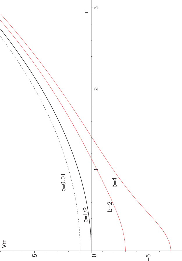
For $M>M_{m}$ we have the ‘Schwarzschild-like’ (S) type. This type of black hole is characterized by the existence of a spacelike singularity and possesses one horizon. The characteristic behaviour of $f$ is displayed in Fig. 11 by (red) solid lines. The ‘Reissner–Nördstrom’ (RN) type is characterized by $M<M_{m}$. Similar to the Reissner–Nördstrom solution, this may have zero, one, or two horizons, see Fig. 11 and Fig. 12. The case $M=M_{m}$ is the ‘marginal’ case, for which function $f_{m}=f(M_{m})$ approaches the (finite) value $f_{m}(0)=1-2bQ$. When this is positive, i.e., for $bQ\leq\frac{1}{2}\,,$ the RN phase describes a naked singularity and the only possible black hole solution is the S-type for $M>M_{m}$. On the other hand when

$$bQ>\frac{1}{2}\,,$$

(74)

the RN-type describes a black hole for $M_{ex}\leq M<M_{m}$, with $M_{ex}$ being the mass of the extremal RN-type black hole, determined from $V(r=r_{ex})=0$, with $r_{ex}$ given by

$$1+\left(2b^{2}+\frac{3}{l^{2}}\right)r_{ex}^{2}-2b\sqrt{r_{ex}^{4}b^{2}+Q^{2}}=0\,.$$

(75)

We gather the possibilities for BI-AdS black holes in the following table; the corresponding dependence of $r_{+}$ on $M/M_{m}$ is depicted in Fig. 13:

$$\begin{array}[]{|c|c|c|}\hline\cr\vrule\lx@intercol\hfil\mbox{BI-AdS black holes}\hfil\lx@intercol\vrule\lx@intercol\\ \hline\cr\mbox{Condition(s)}&\mbox{Type}&\mbox{\# horizons}\\ \hline\cr M>M_{m}&\mbox{S}&\mbox{one}\\ \hline\cr M_{ex}<M<M_{m}&\mbox{RN}&\mbox{two}\\ bQ>\frac{1}{2}&&\\ \hline\cr M=M_{ex}<M_{m}&\mbox{RN}&\mbox{one}\\ bQ>\frac{1}{2}&\mbox{(extremal)}&\\ \hline\cr\end{array}$$

(76)

In all other cases we have a naked singularity.

Let us stress that $M_{m}$ depends on $b$ and $Q$, whereas $M_{ex}=M_{ex}(b,Q,l)$. Therefore, for example, $M_{ex}<M_{m}$ imposes a nontrivial restriction on the parameters of the solution. We also emphasize that the possibility of S-type BI-AdS black holes is sometimes completely ignored in a consideration of BI-AdS black hole thermodynamics [26]. We shall see that it is the S-type black holes for which the most interesting behaviour occurs.

The Smarr relation follows from the first law of black hole thermodynamics and a scaling dimensional argument [5]. [See also [27] for a generalization to the Lovelock gravities.] Beginning with Euler’s theorem (for simplicity formulated only for two variables): given a function $g(x,y)$ such that $g(\alpha^{p}x,\alpha^{q}y)=\alpha^{r}g(x,y)$, it follows that

$$rg(x,y)=px\left(\frac{\partial g}{\partial x}\right)+qy\left(\frac{\partial g}{\partial y}\right)\,.$$

(77)

To obtain the proper scaling relations, for the Born–Infeld case we must consider the mass of the black hole $M$ to be a function of entropy, pressure, angular momentum, charge, and Born–Infeld parameter $b$, $M=M(S,P,J,Q,b)$. Performing the dimensional analysis, we find $[M]=L\,,\ [S]=L^{2}\,,\ [P]=L^{-2}\,,\ [J]=L^{2}\,,\ [Q]=L\,,\ [b]=[E]=L^{-1}\,.$ Since $b$ is a dimensionful parameter, the corresponding term will inevitably appear in the Smarr formula. It is also natural to include its variation in the first law. Hence we have

	$\displaystyle M$	$\displaystyle=$	$\displaystyle 2S\left(\frac{\partial M}{\partial S}\right)-2P\left(\frac{\partial M}{\partial P}\right)+2J\left(\frac{\partial M}{\partial J}\right)$		(78)
			$\displaystyle+Q\left(\frac{\partial M}{\partial Q}\right)-b\left(\frac{\partial M}{\partial b}\right)\,.$

Defining further a quantity conjugate to $b$,

$${\cal B}=\left(\frac{\partial M}{\partial b}\right)\,,$$

(79)

the first law takes the form³³ 3 In fact, this form of the first law remains to be proved. In order to do so, one could, for example, employ the Hamiltonian perturbation theory techniques, similar to [27].

$$dM=TdS+VdP+\Omega dJ+\Phi dQ+{\cal B}db\,.$$

(80)

Using this and Eq. (78), we find the following generalized Smarr formula for stationary Born–Infeld-AdS black holes:

$$M=2(TS-VP+\Omega J)+\Phi Q-{\cal B}b\,.$$

(81)

Let us emphasize that even in the case when the cosmological constant $\Lambda$ and the parameter $b$ are not varied in the first law, i.e., we have $dM=TdS+\Omega dJ+\Phi dQ$, the Smarr relation (81) is valid and the $VP$ and $b{\cal B}$ terms therein are necessary for it to hold. This resolves the problem of inconsistency of the first law and the corresponding Smarr relation raised by Rasheed [28]; see also [29, 30].

In particular, for our (static) black hole solution (69) we have the following thermodynamic quantities: The black hole temperature and the corresponding entropy are

	$\displaystyle T$	$\displaystyle=$	$\displaystyle\frac{1}{4\pi r_{+}}\!\left[1\!+\!\frac{3r_{+}^{2}}{l^{2}}\!+\!2b^{2}r_{+}^{2}\Bigl(1\!-\!\sqrt{1\!+\!\frac{Q^{2}}{b^{2}r_{+}^{4}}}\Bigr)\right],\quad$		(82)
	$\displaystyle S$	$\displaystyle=$	$\displaystyle\frac{A}{4}\,,\quad A=4\pi r_{+}^{2}\,.$		(83)

The thermodynamic volume $V$ and the corresponding pressure $P$ are

$$V=\frac{4}{3}\pi r_{+}^{3}\,,\quad P=-\frac{1}{8\pi}\Lambda=\frac{3}{8\pi}\frac{1}{l^{2}}\,.$$

(84)

The electric potential $\Phi$, measured at infinity with respect to the horizon, is

$$\Phi=\int_{r_{+}}^{\infty}\frac{Qdx}{\sqrt{x^{4}+Q^{2}/b^{2}}}=\frac{Q}{r_{+}}\,{}_{2}F_{1}\!\left(\frac{1}{4},\frac{1}{2};\frac{5}{4};-\frac{Q^{2}}{b^{2}r_{+}^{4}}\right)\,.$$

(85)

Using the first law (80) and the formula (152), we get the following expression for the quantity ${\cal B}$:

	$\displaystyle{\cal B}$	$\displaystyle=$	$\displaystyle\frac{2}{3}br_{+}^{3}-\frac{2}{3}br_{+}^{3}\sqrt{1+\frac{Q^{2}}{b^{2}r_{+}^{4}}}+\frac{Q^{2}}{3br_{+}\sqrt{1+\frac{Q^{2}}{b^{2}r_{+}^{4}}}}$		(86)
			$\displaystyle+\frac{2}{15}\frac{Q^{4}}{b^{3}r_{+}^{5}}\,{}_{2}F_{1}\left(\frac{5}{4},\frac{3}{2};\frac{9}{4};-\frac{Q^{2}}{b^{2}r_{+}^{4}}\right)\,.$

Alternatively, one could calculate ${\cal B}$ from the Smarr formula (81), getting

$${\cal B}=\frac{2}{3}br_{+}^{3}\Bigl(1-\sqrt{1\!+\!\frac{Q^{2}}{b^{2}r_{+}^{4}}}\Bigr)+\frac{Q^{2}}{3br_{+}}\,{}_{2}F_{1}\!\left(\frac{1}{4},\frac{1}{2};\frac{5}{4};-\frac{Q^{2}}{b^{2}r_{+}^{4}}\right)\!.$$

(87)

The two expressions of course coincide and are related by (153). We shall return to this quantity later in this section.

References

- [1] S. Hawking and D. N. Page, Thermodynamics of Black Holes in anti-De Sitter Space, Commun.Math.Phys. 87 (1983) 577.
- [2] A. Chamblin, R. Emparan, C. Johnson, and R. Myers, Charged AdS black holes and catastrophic holography, Phys.Rev. D60 (1999) 064018, [hep-th/9902170].
- [3] A. Chamblin, R. Emparan, C. Johnson, and R. Myers, Holography, thermodynamics and fluctuations of charged AdS black holes, Phys.Rev. D60 (1999) 104026, [hep-th/9904197].
- [4] D. Kubiznak and R. B. Mann, P-V criticality of charged AdS black holes, JHEP 1207 (2012) 033, [arXiv:1205.0559].
- [5] D. Kastor, S. Ray, and J. Traschen, Enthalpy and the Mechanics of AdS Black Holes, Class.Quant.Grav. 26 (2009) 195011, [arXiv:0904.2765].
- [6] B. Dolan, The cosmological constant and the black hole equation of state, Class.Quant.Grav. 28 (2011) 125020, [arXiv:1008.5023].
- [7] B. P. Dolan, Pressure and volume in the first law of black hole thermodynamics, Class.Quant.Grav. 28 (2011) 235017, [arXiv:1106.6260].
- [8] B. P. Dolan, Compressibility of rotating black holes, Phys.Rev. D84 (2011) 127503, [arXiv:1109.0198].
- [9] M. Cvetic, G. Gibbons, D. Kubiznak, and C. Pope, Black Hole Enthalpy and an Entropy Inequality for the Thermodynamic Volume, Phys.Rev. D84 (2011) 024037, [arXiv:1012.2888].
- [10] B. P. Dolan, Where is the PdV term in the first law of black hole thermodynamics?, to appear in Open Questions in Cosmology, ed. Gonzalo J. Olmo, InTech (2012) [arXiv:1209.1272].
- [11] C. Peca and J. Lemos, Thermodynamics of Reissner-Nordstrom anti-de Sitter black holes in the grand canonical ensemble, Phys.Rev. D59 (1999) 124007, [gr-qc/9805004].
- [12] C. Niu, Y. Tian, and X.-N. Wu, Critical Phenomena and Thermodynamic Geometry of RN-AdS Black Holes, Phys.Rev. D85 (2012) 024017, [arXiv:1104.3066].
- [13] R. B. Mann, Misner string entropy, Phys.Rev. D60 (1999) 104047, [hep-th/9903229].
- [14] R. Emparan, C. V. Johnson, and R. Myers, Surface terms as counterterms in the AdS / CFT correspondence, Phys.Rev. D60 (1999) 104001, [hep-th/9903238].
- [15] R. B. Mann and S. F. Ross, Cosmological production of charged black holes pairs, Phys. Rev. D 52 (1995) 2254, [gr-qc/9504015].
- [16] M. M. Caldarelli, G. Cognola, and D. Klemm, Thermodynamics of Kerr-Newman-AdS black holes and conformal field theories, Class.Quant.Grav. 17 (2000) 399–420, [hep-th/9908022].
- [17] S. W. Hawking, C. J. Hunter, and M. M. Taylor-Robinson, Rotation and the AdS/CFT correspondence, Phys. Rev. D59 (1999) 064005, [hep-th/9811056].
- [18] M. Banados, C. Teitelboim, and J. Zanelli, The Black hole in three-dimensional space-time, Phys. Rev. Lett. 69 (1992) 1849–1851, [hep-th/9204099].
- [19] C. Martinez, C. Teitelboim, and J. Zanelli, Charged rotating black hole in three space-time dimensions, Phys.Rev. D61 (2000) 104013, [hep-th/9912259].
- [20] M. Born and L. Infeld, Foundations of the new field theory, Proc. Roy. Soc. A144 (1934) 425.
- [21] G. W. Gibbons, Aspects of Born-Infeld theory and string / M theory, Rev.Mex.Fis. 49S1 (2003) 19–29, [hep-th/0106059].
- [22] S. Fernando and D. Krug, Charged black hole solutions in Einstein-Born-Infeld gravity with a cosmological constant, Gen.Rel.Grav. 35 (2003) 129–137, [hep-th/0306120].
- [23] T. K. Dey, Born-Infeld black holes in the presence of a cosmological constant, Phys.Lett. B595 (2004) 484–490, [hep-th/0406169].
- [24] R.-G. Cai, D.-W. Pang, and A. Wang, Born-Infeld black holes in (A)dS spaces, Phys.Rev. D70 (2004) 124034, [hep-th/0410158].
- [25] S. Fernando, Thermodynamics of Born-Infeld-anti-de Sitter black holes in the grand canonical ensemble, Phys.Rev. D74 (2006) 104032, [hep-th/0608040].
- [26] Y. S. Myung, Y.-W. Kim, and Y.-J. Park, Thermodynamics and phase transitions in the Born-Infeld-anti-de Sitter black holes, Phys.Rev. D78 (2008) 084002, [arXiv:0805.0187].
- [27] D. Kastor, S. Ray, and J. Traschen, Smarr Formula and an Extended First Law for Lovelock Gravity, Class.Quant.Grav. 27 (2010) 235014, [arXiv:1005.5053].
- [28] D. Rasheed, Nonlinear electrodynamics: Zeroth and first laws of black hole mechanics, hep-th/9702087.
- [29] N. Breton, Smarr’s formula for black holes with non-linear electrodynamics, Gen.Rel.Grav. 37 (2005) 643–650, [gr-qc/0405116].
- [30] W. Yi-Huan, Energy and first law of thermodynamics for BornInfeld AdS black hole, Chinese Phys. B19 (2010) 090404.
- [31] R. Banerjee, S. Ghosh, and D. Roychowdhury, New type of phase transition in Reissner Nordstrom - AdS black hole and its thermodynamic geometry, Phys.Lett. B696 (2011) 156–162, [arXiv:1008.2644].
- [32] A. Lala and D. Roychowdhury, Ehrenfest’s scheme and thermodynamic geometry in Born-Infeld AdS black holes, arXiv:1111.5991.
- [33] R. Banerjee and D. Roychowdhury, Critical phenomena in Born-Infeld AdS black holes, Phys.Rev. D85 (2012) 044040, [arXiv:1111.0147].
- [34] R. Banerjee and D. Roychowdhury, Critical behavior of Born Infeld AdS black holes in higher dimensions, Phys.Rev. D85 (2012) 104043, [arXiv:1203.0118].
- [35] O. Miskovic and R. Olea, Thermodynamics of Einstein-Born-Infeld black holes with negative cosmological constant, Phys.Rev. D77 (2008) 124048, [arXiv:0802.2081].
- [36] H. Zhang and X.-Z. Li, Critical exponents of gravity with quantum perturbations, arXiv:1208.0106.
- [37] N. Goldenfeld, Lectures on Phase Transitions and the Renormalization Group. Westview Press, New York, 1992.