跳到论文正文
W Papers独立论文阅读器 arXiv:1208.6178 论文正文 计算阅读时间 · 0%
引用这篇论文根据当前论文元数据生成,正式投稿前建议核对。


License: arXiv.org perpetual non-exclusive license
arXiv:1208.6178v2 [math.DS] 20 Dec 2012

A dynamical approach to Maass cusp formsThanks: The author was supported by the ERC Starting Grant ANTHOS

Anke D. Pohl Address: Mathematisches Institut, Georg-August-Universität Göttingen, Bunsenstr. 3-5, 37073 Göttingen Email address: pohl@uni-math.gwdg.de
Abstract.

For nonuniform cofinite Fuchsian groups Γ\Gamma which satisfy a certain additional geometric condition, we show that the Maass cusp forms for Γ\Gamma are isomorphic to 11-eigenfunctions of a finite-term transfer operator. The isomorphism is constructive.

Key words and phrases: 
Maass cusp forms, transfer operator, period functions, symbolic dynamics, geodesic flow
2010 Mathematics Subject Classification
Primary: 11F37, 37C30; Secondary: 37B10, 37D35, 37D40, 11F67

1. Introduction

Let Γ\Gamma be a nonuniform cofinite Fuchsian group and consider its action on the hyperbolic plane ℍ\mathbb{H} by Möbius transformations. The purpose of this article is to characterize, under a certain additional geometric requirement on Γ\Gamma, the Maass cusp forms for Γ\Gamma as 11-eigenfunctions of a finite-term transfer operator which arises from a discretization of the geodesic flow on Γ\ℍ\Gamma\backslash\mathbb{H}.

Maass cusp forms for Γ\Gamma are specific eigenfunctions of the Laplace-Beltrami operator Δ\Delta acting on L2​(Γ\ℍ)L^{2}(\Gamma\backslash\mathbb{H}) which decay rapidly towards any cusp of Γ\ℍ\Gamma\backslash\mathbb{H}. They span the cuspidal spectrum of Δ\Delta in L2​(Γ\ℍ)L^{2}(\Gamma\backslash\mathbb{H}), which together with the residual spectrum spans the discrete spectrum. These forms play important roles in various fields, e.g. harmonic analysis, number theory, mathematical physics and quantum chaos. For lattices with special symmetries (e.g. congruence subgroups), infinitely many linearly independent Maass cusp forms are known to exist, even though only few could be provided by explicit formulas, yet. For generic nonuniform lattices, according to the Phillips-Sarnak conjecture [PS85a, PS85b], existence of Maass cusp forms is expected to be very limited.

The transfer operator approach has its origin in thermodynamic formalism and was initially primarily used to investigate dynamical zeta functions [Rue94, Rue02]. An important example of such a dynamical zeta function is the Selberg zeta function

Z⁡(s):=∏γ∏k=0∞(1−e−(s+k)​ℓ​(γ)),Z(s)\mathrel{\mathop{:}}=\prod_{\gamma}\prod_{k=0}^{\infty}\left(1-e^{-(s+k)\ell(\gamma)}\right),

converging on some right halfplane. Here, the outer product runs over all primitive periodic geodesics γ\gamma on Γ\ℍ\Gamma\backslash\mathbb{H}, and ℓ⁡(γ)\ell(\gamma) denotes the length of γ\gamma. As known from classical Selberg theory, the Selberg zeta function encodes the eigenvalues of Maass cusp forms in some of the zeros of its meromorphic continuation. In terms of quantum chaos, the Selberg zeta function allows to correlate some properties of some quantum objects (eigenvalues of Maass cusp forms) with some properties of purely classical objects (geodesic length spectrum).

For the modular surface PSL2⁡(ℤ)\ℍ\PSL_{2}(\mathbb{Z})\backslash\mathbb{H}, a deeper relation has been established by the following transfer operator approach. Mayer [May76, May90, May91] showed that the transfer operator ℒs\mathcal{L}_{s} with parameter s∈ℂs\in\mathbb{C} of the Gauss map,

ℒs​f​(z)=∑n∈ℕ1(z+n)2​s​f​(1z+n),\mathcal{L}_{s}f(z)=\sum_{n\in\mathbb{N}}\frac{1}{(z+n)^{2s}}f\left(\frac{1}{z+n}\right),

is a nuclear operator of order zero on a certain Banach space of holomorphic functions, its Fredholm determinant represents the Selberg zeta function

(1) Z⁡(s)=det(1−ℒs2)=det(1−ℒs)​det(1+ℒs)Z(s)=\det(1-\mathcal{L}_{s}^{2})=\det(1-\mathcal{L}_{s})\det(1+\mathcal{L}_{s})

on some right halfplane Re⁡s>s0\Rea s>s_{0}, and the family (ℒs)Re⁡s>s0(\mathcal{L}_{s})_{\Rea s>s_{0}} admits a meromorphic continuation to all s∈ℂs\in\mathbb{C}. The Gauss map and hence the transfer operator arise from a specific discretization of the geodesic flow on the modular surface [Art24, Ser85]. The ±1\pm 1-eigenfunctions of ℒs\mathcal{L}_{s} (1>Re⁡s>01>\Rea s>0) are isomorphic to highly regular solutions of the functional equation [CM99, LZ01]

(2) f⁡(x)=f⁡(x+1)+(x+1)−2​s​f​(xx+1),x∈ℝ>0.f(x)=f(x+1)+(x+1)^{-2s}f\left(\frac{x}{x+1}\right),\quad x\in\mathbb{R}_{>0}.

By Lewis-Zagier [LZ01] (see [Bru97] for an alternative approach, and [Lew97] for an earlier result on even Maass cusp forms), these solutions are isomorphic to the Maass cusp forms for PSL2⁡(ℤ)\PSL_{2}(\mathbb{Z}) with eigenvalue s⁡(1−s)s(1-s). The factorization in (1) relates to even resp. odd Maass cusp forms (see [Efr93] for a spectral result prior to [LZ01]). Hence, in this approach, Maass cusp forms themselves, not only their eigenvalues, can be recovered from the geodesic flow. In addition, the meromorphic continuation of the Selberg zeta function and the relation between its zeros and the eigenvalues of Maass cusp forms can be rededuced. However, the functional equation of ZZ could not be found via transfer operators, yet. The solutions to (2) of sufficient regularity were coined period functions in [LZ01], in analogy to period polynomials in the Eichler-Manin-Shimura theory.

In the sequel, also other automorphic forms for PSL2⁡(ℤ)\PSL_{2}(\mathbb{Z}) could be included into this picture [CM98, CM99].

Up to date, the complete picture from a representation of the Selberg zeta function as a Fredholm determinant of a transfer operator family via period functions to Maass cusp forms could only be extended to some finite index subgroups of PSL2⁡(ℤ)\PSL_{2}(\mathbb{Z}) [DH07, CM01a, CM01b, HMM05, FMM07]. Moreover, there is a second transfer operator approach to PSL2⁡(ℤ)\PSL_{2}(\mathbb{Z}) [MMS12, BM09] using the discretization in [MS08]. From the point of view of quantum chaos, the most significant component of such a transfer operator approach is to establish that certain eigenfunctions of the transfer operator are isomorphic to Maass cusp forms. The discretization in [Poh10] for the geodesic flow on Γ\ℍ\Gamma\backslash\mathbb{H} for various subgroups Γ\Gamma of PSL2⁡(ℝ)\PSL_{2}(\mathbb{R}) has been developed specifically for such a “short-cut” transfer operator approach to Maass cusp forms. Common to the approaches mentioned above is that the transfer operators involve infinitely many terms. In contrast, the transfer operators arising from [Poh10] are finite-term. More precisely, the transfer operator with parameter s∈ℂs\in\mathbb{C} is given by a finite sum of specific elements of Γ\Gamma acting via the action of principal series representation with spectral parameter ss on functions which are defined on certain intervals in the geodesic boundary of ℍ\mathbb{H}. It is shown in [MP11] for Hecke triangle groups and in [Poh12] for Γ0​(p)\Gamma_{0}(p), pp prime, that the 11-eigenfunctions of these transfer operators for these lattices are period functions and are isomorphic to Maass cusp forms via an integral transform, taking advantage of the characterization of Maass cusp forms in parabolic 11-cohomology in [BLZ12]. The functional equations replacing (2) are just the defining equations for 11-eigenfunctions of these transfer operators. Moreover, for Hecke triangle groups, [MP11] shows a representation of the Selberg zeta function as in (1), including the factorization, for certain modified transfer operators. In [Poh], a spectral result analogous to [Efr93] is provided.

Here we generalize the dynamical approach to Maass cusp forms to nonuniform lattices Γ\Gamma in PSL2⁡(ℝ)\PSL_{2}(\mathbb{R}), which satisfy a certain additional geometric requirement. Our main result is as follows:

Theorem A.

Let s∈ℂs\in\mathbb{C}, 0<Re⁡s<10<\Rea s<1. Then the space of Maass cusp forms for Γ\Gamma with eigenvalue s⁡(1−s)s(1-s) is isomorphic to the space of sufficiently regular 11-eigenfunctions of the transfer operator with parameter ss.

The regularity required for the eigenfunctions is specified in Theorem 3.1 below. For the proof of Theorem A we use the characterization of Maass cusp forms in parabolic 11-cohomology in [BLZ12] and show that the parabolic 11-cocycle classes are isomorphic to these highly regular 11-eigenfunctions of the transfer operator. Both of these isomorphisms are constructive, and hence the isomorphism in Theorem A is so.

The discretization of the geodesic flow allows for a number of choices, each choice giving rise to a definition of period functions. By Theorem A, all these spaces of period functions are isomorphic. The precise effect of the choices in the discretization is discussed in Section 4 below, where we also provide an explicit formula for the isomorphism between the different spaces of period functions.

In Section 2 below we recall the discretization of the geodesic flow, present the associated transfer operators and the definition of period functions, and provide the necessary background on the parabolic 11-cohomology characterization of Maass cusp forms. Theorem A is then proved in Section 3.

We provide an ongoing example to illustrate all constructions. Other examples can be found in [Poh10, HP08, MP11, Poh12].

A representation as in (1) of the Selberg zeta function as a Fredholm determinant of a transfer operator family (not necessarily with a factorization) could be established for various lattices Γ\Gamma in PSL2⁡(ℝ)\PSL_{2}(\mathbb{R}) [Pol91, Fri96, Mor97, CM01b, MMS12, MP11], using several discretization for the geodesic flow on Γ\ℍ\Gamma\backslash\mathbb{H}. In some approaches, the representation is not exact. It rather requires a “correction factor” which accounts for double-coding in the discretization [Pol91, Mor97, MMS12]. We expect that the transfer operator families used in the article at hand allow for a similar modification as in [MP11], but we leave this for future investigations.

Concerning period functions, in addition to the already mentioned results from [DH07, CM01b, BLZ12, MP11, Poh12], the 11-eigenfunctions of the (infinite-term) transfer operators for Hecke triangle groups in [MMS12] are shown there to satisfy finite-term functional equations. However, for Hecke triangle groups other than PSL2⁡(ℤ)\PSL_{2}(\mathbb{Z}), their relation to Maass cusp forms is still an open problem. In Section 4 we compare our period functions to these results.

Acknowledgment. The author thanks the referee for helpful comments.

2. Symbolic dynamics, transfer operators, and period functions

This section serves to present the additional geometric condition required of the considered Fuchsian lattices Γ\Gamma and to briefly recall the discretization of the geodesic flow on Γ\ℍ\Gamma\backslash\mathbb{H} from [Poh10] as well as the characterization of Maass cusp forms in parabolic 11-cohomology from [BLZ12]. For proofs we refer to the original articles. Moreover, we provide a definition of period functions.

To simplify the exposition, we use the upper half plane

ℍ:={z∈ℂ∣Im⁡z>0}\mathbb{H}\mathrel{\mathop{:}}=\{z\in\mathbb{C}\mid\Ima z>0\}

as model for the hyperbolic plane and identify its geodesic boundary with P1​(ℝ)≅ℝ∪{∞}P^{1}(\mathbb{R})\cong\mathbb{R}\cup\{\infty\}. In this model, the group of orientation-preserving Riemannian isometries on ℍ\mathbb{H} can be identified with PSL2⁡(ℝ)\PSL_{2}(\mathbb{R}), whose action on ℍ\mathbb{H} is given by fractional linear transformations and extends continuously to P1​(ℝ)P^{1}(\mathbb{R}). Thus we have

[abcd].z={a​z+bc​z+dif c​z+d≠0∞if c​z+d=0and[abcd].∞={acif c≠0∞if c=0\begin{bmatrix}a&b\\ c&d\end{bmatrix}.z=\begin{cases}\frac{az+b}{cz+d}&\text{if $cz+d\not=0$}\\ \infty&\text{if $cz+d=0$}\end{cases}\quad\text{and}\quad\begin{bmatrix}a&b\\ c&d\end{bmatrix}.\infty=\begin{cases}\frac{a}{c}&\text{if $c\not=0$}\\ \infty&\text{if $c=0$}\end{cases}

for [abcd]∈PSL⁡(2,ℝ)\left[\begin{smallmatrix}a&b\\ c&d\end{smallmatrix}\right]\in\PSL(2,\mathbb{R}) and z∈ℍ∪ℝz\in\mathbb{H}\cup\mathbb{R}. Throughout let Γ\Gamma be a nonuniform cofinite Fuchsian group and suppose that ∞\infty is a representative of a cusp of Γ\ℍ\Gamma\backslash\mathbb{H}. Then the stabilizer group Γ∞=StabΓ⁡(∞)\Gamma_{\infty}=\Stab_{\Gamma}(\infty) of ∞\infty in Γ\Gamma is generated by some element

T:=[1λ01]∈ΓT\mathrel{\mathop{:}}=\begin{bmatrix}1&\lambda\\ 0&1\end{bmatrix}\quad\in\Gamma

with λ>0\lambda>0. A point in P1​(ℝ)P^{1}(\mathbb{R}) is called cuspidal if it is fixed by a parabolic element in Γ\Gamma. We use S​ℍS\mathbb{H} to denote the unit tangent bundle of ℍ\mathbb{H}. The action of Γ\Gamma extends to S​ℍS\mathbb{H}. By Γ\ℍ\Gamma\backslash\mathbb{H} resp. Γ\S​ℍ\Gamma\backslash S\mathbb{H} we denote the quotient space of the Γ\Gamma-action on ℍ\mathbb{H} resp. S​ℍS\mathbb{H}. We remark that we may identify the unit tangent bundle of Γ\ℍ\Gamma\backslash\mathbb{H} with Γ\S​ℍ\Gamma\backslash S\mathbb{H}. If UU is a subset of ℍ\mathbb{H}, then we let ∂U\partial U denote its boundary. The complement of a set BB in a set AA is denoted by

A∖B={a∈A∣a∉B}.A\smallsetminus B=\{a\in A\mid a\notin B\}.

Finally, a smooth function always refers to a C∞C^{\infty} function.

2.1. The additional requirement on Γ\Gamma

The additional condition we require to be satisfied by Γ\Gamma is of geometric nature and restricts the admissible boundary structure of the subset of ℍ\mathbb{H} which is common to all exteriors of isometric spheres of Γ\Gamma. In short, it says that there is a Ford fundamental domain for Γ\Gamma constructed with respect to ∞\infty such that the highest points of all non-vertical bounding complete geodesic segments are contained in the boundary of the fundamental domain but are not intersection points of two non-vertical sides of the fundamental domain.

Let g=[abcd]∈Γ∖Γ∞g=\left[\begin{smallmatrix}a&b\\ c&d\end{smallmatrix}\right]\in\Gamma\smallsetminus\Gamma_{\infty}. Then the isometric sphere of gg is the set

I⁡(g):={z∈ℍ∣|c​z+d|=1}.I(g)\mathrel{\mathop{:}}=\{z\in\mathbb{H}\mid|cz+d|=1\}.

It is identical to the complete geodesic segment connecting −d−1c\frac{-d-1}{c} and −d+1c\frac{-d+1}{c}, or the semi-circle in ℍ\mathbb{H} with center −dc-\frac{d}{c} and radius 1|c|\frac{1}{|c|}. The exterior of I⁡(g)I(g) is

ext⁡I⁡(g):={z∈ℍ∣|c​z+d|>1}.\Ext I(g)\mathrel{\mathop{:}}=\{z\in\mathbb{H}\mid|cz+d|>1\}.

The summit of I⁡(g)I(g) is the point

s=−dc+i|c|∈ℍ.s=-\frac{d}{c}+\frac{i}{|c|}\quad\in\mathbb{H}.

Let

𝒦:=⋂g∈Γ∖Γ∞ext⁡I⁡(g)\mathcal{K}\mathrel{\mathop{:}}=\bigcap_{g\in\Gamma\smallsetminus\Gamma_{\infty}}\Ext I(g)

be the common part of all exteriors of the isometric spheres of Γ\Gamma. This is a convex subset of ℍ\mathbb{H} which contains

{z∈ℍ∣Im⁡z>y0}\{z\in\mathbb{H}\mid\Ima z>y_{0}\}

for a sufficiently large y0>0y_{0}>0 and whose boundary is a locally finite union of geodesic segments which are connected subsets of isometric spheres. An isometric sphere of Γ\Gamma is called relevant if it coincides with the boundary of 𝒦\mathcal{K} in more than one point. From now on we impose the following condition on Γ\Gamma:

(A) If for g∈Γ∖Γ∞g\in\Gamma\smallsetminus\Gamma_{\infty} the isometric sphere I⁡(g)I(g) is relevant, then its summit is contained in ∂𝒦\partial\mathcal{K} but is not a vertex of 𝒦\mathcal{K}.

For r∈ℝr\in\mathbb{R}, let ℱ∞​(r):=(r,r+λ)+i​ℝ>0\mathcal{F}_{\infty}(r)\mathrel{\mathop{:}}=(r,r+\lambda)+i\mathbb{R}_{>0}. Then

ℱ⁡(r):=ℱ∞​(r)∩𝒦\mathcal{F}(r)\mathrel{\mathop{:}}=\mathcal{F}_{\infty}(r)\cap\mathcal{K}

is a Ford fundamental domain for Γ\Gamma. If we choose for rr the center of a relevant isometric sphere, then ℱ⁡(r)\mathcal{F}(r) is a fundamental domain as described above.

Example 2.1.

Condition (A) is satisfied by several Fuchsian lattices. One such lattice is provided in Example 2.2, which we will use as an ongoing example for all constructions. Other lattices satisfying (A) are e.g. Hecke triangle groups and various congruence subgroups. In the following we present a lattice which does not satisfy (A).

Let Λ\Lambda be the lattice in PSL2⁡(ℝ)\PSL_{2}(\mathbb{R}) which is generated by the three elements

(1171101),(18−511−3)and(3−1103).\begin{pmatrix}1&\frac{17}{11}\\ 0&1\end{pmatrix},\quad\begin{pmatrix}18&-5\\ 11&-3\end{pmatrix}\quad\text{and}\quad\begin{pmatrix}3&-1\\ 10&3\end{pmatrix}.

A Ford fundamental domain for Λ\Lambda is displayed in Figure 1. We refer to [Poh10] for proofs. It clearly shows that (A) does not hold for Λ\Lambda.

Refer to caption
Figure 1. Ford fundamental domain for Λ\Lambda

2.2. Discretization

The starting point in [Poh10] for the discretization of the geodesic flow on Γ\ℍ\Gamma\backslash\mathbb{H} is a specific choice of a cross section in the sense of Poincaré for this flow. This cross section is a subset C^\widehat{C} on the unit tangent bundle Γ\S​ℍ\Gamma\backslash S\mathbb{H} of Γ\ℍ\Gamma\backslash\mathbb{H} which is intersected by almost all geodesics infinitely often in the past and the future, and each such intersection is discrete in time. Geodesics are here parametrized by arc length, and “almost all” refers to all geodesics which do not converge to a cusp forward or backward in time. Before we expound the construction of C^\widehat{C} in Section 2.3 below, we briefly explain how it gives rise to a discrete dynamical system on subsets of ℝ\mathbb{R}.

For v^∈C^\widehat{v}\in\widehat{C} let γ^v\widehat{\gamma}_{v} denote the geodesic on Γ\ℍ\Gamma\backslash\mathbb{H} determined by

dd​t|t=0​γ^v​(t)=v^.\frac{d}{dt}|_{t=0}\widehat{\gamma}_{v}(t)=\widehat{v}.

The choice of C^\widehat{C} yields that if γ^v\widehat{\gamma}_{v} does not converge to a cusp, there is a minimal return time of γ^v\widehat{\gamma}_{v} to C^\widehat{C}, that is a minimal time t⁡(v^)>0t(\widehat{v})>0 such that

dd​t|t=t⁡(v^)​γ^v​(t)∈C^.\frac{d}{dt}|_{t=t(\widehat{v})}\widehat{\gamma}_{v}(t)\in\widehat{C}.

Therefore C^\widehat{C} induces the (partially defined) first return map

ℛ:C^→C^,v^↦dd​t|t=t⁡(v^)​γ^v​(t).\mathcal{R}\colon\widehat{C}\to\widehat{C},\quad\widehat{v}\mapsto\frac{d}{dt}|_{t=t(\widehat{v})}\widehat{\gamma}_{v}(t).

The precise domain of definition for ℛ\mathcal{R} is discussed in detail in [Poh10]. The sole property of this domain used hiddenly here is its density in C^\widehat{C}.

A major property of the cross section C^\widehat{C} is that it has a set of representatives C′C^{\prime} in S​ℍS\mathbb{H} which decomposes (uniquely) into a finite number C1′,…,Ck′C^{\prime}_{1},\ldots,C^{\prime}_{k} of subsets each of which is either of the form

Cj′={X∈Sℍ|X=a∂∂x|rj+i​y+b∂∂y|rj+i​y,a>0,b∈ℝ,y>0}C^{\prime}_{j}=\left\{X\in S\mathbb{H}\left|\ X=a\frac{\partial}{\partial x}|_{r_{j}+iy}+b\frac{\partial}{\partial y}|_{r_{j}+iy},\ a>0,\ b\in\mathbb{R},\ y>0\right.\right\}

for some cuspidal point rj∈ℝr_{j}\in\mathbb{R}, or

Cj′={X∈Sℍ|X=a∂∂x|rj+i​y+b∂∂y|rj+i​y,a<0,b∈ℝ,y>0}C^{\prime}_{j}=\left\{X\in S\mathbb{H}\left|\ X=a\frac{\partial}{\partial x}|_{r_{j}+iy}+b\frac{\partial}{\partial y}|_{r_{j}+iy},\ a<0,\ b\in\mathbb{R},\ y>0\right.\right\}

for some cuspidal point rj∈ℝr_{j}\in\mathbb{R}. In other words, each Cj′C^{\prime}_{j} consists of the unit tangent vectors in S​ℍS\mathbb{H} which are based on the complete geodesic segment (rj,∞)(r_{j},\infty) and point into either of the halfspaces {Rez>rj}\{\Rea z>r_{j}\} or {Rez<rj}\{\Rea z<r_{j}\}. For a given subset UU of ℍ\mathbb{H} and a unit tangent vector v∈S​ℍv\in S\mathbb{H}, we say that vv points into UU if the geodesic γv\gamma_{v} determined by

dd​t|t=0​γv​(t)=v\frac{d}{dt}|_{t=0}\gamma_{v}(t)=v

immediately runs into UU. More precisely, if there exists η>0\eta>0 such that γv​((0,η))⊆U\gamma_{v}((0,\eta))\subseteq U.

The combination of this partition of C′C^{\prime} and the first return map ℛ\mathcal{R} allows to define a discrete dynamical system on parts of the geodesic boundary of ℍ\mathbb{H} which is conjugate to ℛ\mathcal{R}. To that end, let

D~j:={(γv(−∞),γv(+∞),j)∣v∈Cj′}for j=1,…,k,\widetilde{D}_{j}\mathrel{\mathop{:}}=\{(\gamma_{v}(-\infty),\gamma_{v}(+\infty),j)\mid v\in C^{\prime}_{j}\}\quad\text{for $j=1,\ldots,k$,}

and

D~:=∐j=1kD~j.\widetilde{D}\mathrel{\mathop{:}}=\coprod_{j=1}^{k}\widetilde{D}_{j}.

Then the map τ:C^→D~\tau\colon\widehat{C}\to\widetilde{D} defined by

τ(v^):=(γv(−∞),γv(+∞),j)if v^ is represented by v∈Cj′\tau(\widehat{v})\mathrel{\mathop{:}}=(\gamma_{v}(-\infty),\gamma_{v}(+\infty),j)\quad\text{if $\widehat{v}$ is represented by $v\in C^{\prime}_{j}$}

is a bijection. Thus, there is a unique (partially defined) self-map F~\widetilde{F} on D~\widetilde{D} which is conjugate to ℛ\mathcal{R} via τ\tau. Its domain of definition corresponds to the domain of definition of ℛ\mathcal{R}.

For each j∈{1,…,k}j\in\{1,\ldots,k\}, the structure of Cj′C^{\prime}_{j} yields that D~j\widetilde{D}_{j} is either of the form

(−∞,rj)×(rj,∞)×{j}or(rj,∞)×(−∞,rj)×{j}.(-\infty,r_{j})\times(r_{j},\infty)\times\{j\}\quad\text{or}\quad(r_{j},\infty)\times(-\infty,r_{j})\times\{j\}.

As shown in [Poh10], the map F~\widetilde{F} is locally given by Möbius transformations of specific elements from Γ\Gamma.

From the discrete dynamical system (D~,F~)(\widetilde{D},\widetilde{F}) we will only need its expanding direction, which means its projection to the last two components. We denote this restricted discrete dynamical system with (D,F)(D,F), where

D:=∐j=1kDj,Dj:={(γv(∞),j)∣v∈Cj′}D\mathrel{\mathop{:}}=\coprod_{j=1}^{k}D_{j},\quad D_{j}\mathrel{\mathop{:}}=\{(\gamma_{v}(\infty),j)\mid v\in C^{\prime}_{j}\}

and FF is the self-map of DD which is induced by F~\widetilde{F}. To be precise, FF is a self-map only on

D∖{(r,j)∣r cuspidal, j=1,…,k}D\smallsetminus\{(r,j)\mid\text{$r$ cuspidal, $j=1,\ldots,k$}\}

and can be analytically extended to a map defined on DD up to finitely many points. Here we work with this analytic extension and still write DD for its domain of definition. It will always be clear on which points of DD the map FF is not defined.

2.3. Cross section and choice of set of representatives

For the definition of the cross section C^\widehat{C} and a choice of its set C′C^{\prime} of representatives we consider 𝒦\mathcal{K} as a subset of ℍ∪P1​(ℝ)\mathbb{H}\cup P^{1}(\mathbb{R}).

The vertices of 𝒦\mathcal{K} which are contained in ℍ\mathbb{H} are called inner vertices, those which are contained in ℝ\mathbb{R} are called infinite vertices. We decompose its closure 𝒦¯\overline{\mathcal{K}} as follows into a collection of hyperbolic triangles and rectangles. If v≠∞v\not=\infty is a vertex of 𝒦\mathcal{K}, then vv is either the intersection point or the common endpoint of two (uniquely determined) relevant isometric spheres. Let s1s_{1} resp. s2s_{2} be their summits. If vv is an inner vertex, then we form the hyperbolic rectangle with vertices ∞\infty, s1s_{1}, vv and s2s_{2}. If vv is an infinite vertex, then we form the two hyperbolic triangles with vertices ∞\infty, vv and s1s_{1} resp. ∞\infty, vv and s2s_{2}. In any case, if a side of these triangles and rectangles has ∞\infty as one endpoint, then we call it vertical, otherwise non-vertical. Let 𝒞\mathcal{C} denote this collection of hyperbolic triangles and rectangles.

Let C~\widetilde{C} be the set of unit tangent vectors X∈S​ℍX\in S\mathbb{H} such that XX is based on a vertical side of an element in 𝒞\mathcal{C} but is not tangent to this side. Further let π:S​ℍ→Γ\S​ℍ\pi\colon S\mathbb{H}\to\Gamma\backslash S\mathbb{H} denote the quotient map. Then we choose

C^:=π⁡(C~)\widehat{C}\mathrel{\mathop{:}}=\pi(\widetilde{C})

as cross section for the geodesic flow on Γ\S​ℍ\Gamma\backslash S\mathbb{H}. To find a set of representatives for C^\widehat{C} with the properties announced in Section 2.2 we proceed as follows.

The elements of 𝒞\mathcal{C} (now considered as subsets of ℍ\mathbb{H}) provide a tesselation of ℍ\mathbb{H}. This means their Γ\Gamma-translates cover ℍ\mathbb{H} and, whenever two Γ\Gamma-translates of elements in 𝒞\mathcal{C} have a point in common, then it is either a single point which is a common vertex of both translates or they coincide at a common side or they are equal. Out of the family 𝒞\mathcal{C} we pick a subfamily 𝔸\mathbb{A} of triangles and rectangles whose union forms a (closed) fundamental region for Γ\Gamma in ℍ\mathbb{H}. Within the family 𝔸\mathbb{A}, the tesselation property induces a unique and well-defined side-pairing. In analogy with Poincaré’s Fundamental Polyhedron Theorem we use this side-pairing to define cycles as explained in the following. For this we remark that non-vertical sides of rectangles (resp. triangles) in 𝔸\mathbb{A} can only be paired with non-vertical sides of rectangles (resp. triangles).

Let 𝒜∈𝔸\mathcal{A}\in\mathbb{A} be a rectangle. Suppose that vv is the inner vertex of 𝒦\mathcal{K} to which 𝒜\mathcal{A} is associated, and let b1,b2b_{1},b_{2} denote the two non-vertical sides of 𝒜\mathcal{A}. We denote by k1​(𝒜),k2​(𝒜)k_{1}(\mathcal{A}),k_{2}(\mathcal{A}) the two elements in Γ∖Γ∞\Gamma\smallsetminus\Gamma_{\infty} such that bj∈I⁡(kj​(𝒜))b_{j}\in I(k_{j}(\mathcal{A})) and kj​(𝒜)​bjk_{j}(\mathcal{A})b_{j} is a non-vertical side of some rectangle in 𝔸\mathbb{A}. These are the side-pairing elements for the non-vertical sides of 𝒜\mathcal{A}. We define 𝒜⁡(v):=𝒜\mathcal{A}(v)\mathrel{\mathop{:}}=\mathcal{A}. To any rectangle 𝒜=𝒜⁡(v)∈𝔸\mathcal{A}=\mathcal{A}(v)\in\mathbb{A} and any choice h∈{k1​(𝒜),k2​(𝒜)}h\in\{k_{1}(\mathcal{A}),k_{2}(\mathcal{A})\} we assign a finite sequence in 𝔸×Γ\mathbb{A}\times\Gamma using the following algorithm:

Set v1:=vv_{1}\mathrel{\mathop{:}}=v, 𝒜1:=𝒜⁡(v1)\mathcal{A}_{1}\mathrel{\mathop{:}}=\mathcal{A}(v_{1}), h1:=hh_{1}\mathrel{\mathop{:}}=h, g1:=idg_{1}\mathrel{\mathop{:}}=\id and g2:=h1g_{2}\mathrel{\mathop{:}}=h_{1}. Iteratively for j=2,3,…j=2,3,\ldots set vj:=gj​(v)v_{j}\mathrel{\mathop{:}}=g_{j}(v) and 𝒜j:=𝒜⁡(vj)\mathcal{A}_{j}\mathrel{\mathop{:}}=\mathcal{A}(v_{j}). Let hjh_{j} be the element in Γ∖Γ∞\Gamma\smallsetminus\Gamma_{\infty} such that {hj,hj−1−1}={k1​(𝒜j),k2​(𝒜j)}\{h_{j},h_{j-1}^{-1}\}=\{k_{1}(\mathcal{A}_{j}),k_{2}(\mathcal{A}_{j})\}. Set gj+1:=hj​gjg_{j+1}\mathrel{\mathop{:}}=h_{j}g_{j}. The algorithm stops if gj+1=idg_{j+1}=\id. We assign to (𝒜1,h1)(\mathcal{A}_{1},h_{1}) the sequence (the cycle) ((𝒜j,hj))j=1,…,k\big((\mathcal{A}_{j},h_{j})\big)_{j=1,\ldots,k} where k>2k>2 is minimal such that gk+1=idg_{k+1}=\id.

We consider the two sequences determined by (𝒜,k1​(𝒜))(\mathcal{A},k_{1}(\mathcal{A})) and (𝒜,k2​(𝒜))(\mathcal{A},k_{2}(\mathcal{A})) as equivalent, as well as any sequences determined by any element (𝒜′,h′)(\mathcal{A}^{\prime},h^{\prime}) of these sequences.

Let 𝒜∈𝔸\mathcal{A}\in\mathbb{A} be a triangle and let bb be its non-vertical side. Then there are unique elements h∈Γ∖Γ∞h\in\Gamma\smallsetminus\Gamma_{\infty} and 𝒜′∈𝔸\mathcal{A}^{\prime}\in\mathbb{A} such that b∈I⁡(h)b\in I(h) and h​bhb is the non-vertical side of 𝒜′\mathcal{A}^{\prime}. We assign to (𝒜,h)(\mathcal{A},h) the cycle ((𝒜,h),(𝒜′,h−1))\big((\mathcal{A},h),(\mathcal{A}^{\prime},h^{-1})\big), which we consider to be equivalent to the cycle ((𝒜′,h−1),(𝒜,h))\big((\mathcal{A}^{\prime},h^{-1}),(\mathcal{A},h)\big).

For any of these cycles in 𝔸×Γ\mathbb{A}\times\Gamma we call any element (𝒜,h)(\mathcal{A},h) contained in it a generator of the sequence or its equivalence class. To define a set of representatives C′C^{\prime} for C^\widehat{C} we fix a generator for each equivalence class of cycles. Let 𝕊\mathbb{S} denote the set of chosen generators.

Let (𝒜,h)(\mathcal{A},h) be an element of a cycle in 𝔸×Γ\mathbb{A}\times\Gamma. Then one of the vertical sides of 𝒜\mathcal{A} is contained in the geodesic segment (h−1.∞,∞)(h^{-1}.\infty,\infty). We define

ε⁡(𝒜,h):={+1if 𝒜⊆{z∈ℍ∣Rez≥h−1.∞},−1if 𝒜⊆{z∈ℍ∣Rez≤h−1.∞}.\varepsilon(\mathcal{A},h)\mathrel{\mathop{:}}=\begin{cases}+1&\text{if $\mathcal{A}\subseteq\{z\in\mathbb{H}\mid\Rea z\geq h^{-1}.\infty\}$,}\\ -1&\text{if $\mathcal{A}\subseteq\{z\in\mathbb{H}\mid\Rea z\leq h^{-1}.\infty\}$.}\end{cases}

Let (𝒜,h)∈𝕊(\mathcal{A},h)\in\mathbb{S}. Suppose first that 𝒜\mathcal{A} is a rectangle. Let ((𝒜j,hj))j=1,…,k\big((\mathcal{A}_{j},h_{j})\big)_{j=1,\ldots,k} be the cycle in 𝔸×Γ\mathbb{A}\times\Gamma determined by (𝒜,h)(\mathcal{A},h). Let

cyl⁡(𝒜):=min⁡({ℓ∈{1,…,k−1}∣𝒜ℓ+1=𝒜}∪{k}).\cyl(\mathcal{A})\mathrel{\mathop{:}}=\min\big(\{\ell\in\{1,\ldots,k-1\}\mid\mathcal{A}_{\ell+1}=\mathcal{A}\}\cup\{k\}\big).

For j=1,…,cyl⁡(𝒜)j=1,\ldots,\cyl(\mathcal{A}) we set

C(𝒜,h),j′:={a∂∂x|hj−1.∞+i​y+b∂∂y|hj−1.∞+i​y∈Sℍ|εj⋅a>0,b∈ℝ,y>0}C^{\prime}_{(\mathcal{A},h),j}\mathrel{\mathop{:}}=\left\{a\frac{\partial}{\partial x}|_{h_{j}^{-1}.\infty+iy}+b\frac{\partial}{\partial y}|_{h_{j}^{-1}.\infty+iy}\in S\mathbb{H}\ \left|\ \varepsilon_{j}\cdot a>0,\ b\in\mathbb{R},\ y>0\vphantom{\frac{\partial}{\partial x}|_{h_{j}^{-1}.\infty+iy}}\right.\right\}

where εj:=ε⁡(𝒜j,hj)\varepsilon_{j}\mathrel{\mathop{:}}=\varepsilon(\mathcal{A}_{j},h_{j}). Suppose now that 𝒜\mathcal{A} is a triangle and let ((𝒜,h),(𝒜′,h−1))\big((\mathcal{A},h),(\mathcal{A}^{\prime},h^{-1})\big) be the cycle determined by (𝒜,h)(\mathcal{A},h). Let v,v′∈ℝv,v^{\prime}\in\mathbb{R} be the infinite vertices of 𝒦\mathcal{K} to which 𝒜\mathcal{A} resp. 𝒜′\mathcal{A}^{\prime} are associated. Choose an integer m=m⁡(𝒜,h)∈ℤm=m(\mathcal{A},h)\in\mathbb{Z} and set ε:=ε⁡(𝒜,h)\varepsilon\mathrel{\mathop{:}}=\varepsilon(\mathcal{A},h). We define

C(𝒜,h),1′\displaystyle C^{\prime}_{(\mathcal{A},h),1} :={a∂∂x|v+i​y+b∂∂y|v+i​y∈Sℍ|ε⋅a<0,b∈ℝ,y>0},\displaystyle\mathrel{\mathop{:}}=\left\{a\frac{\partial}{\partial x}|_{v+iy}+b\frac{\partial}{\partial y}|_{v+iy}\in S\mathbb{H}\ \left|\ \varepsilon\cdot a<0,\ b\in\mathbb{R},\ y>0\vphantom{\frac{\partial}{\partial x}|_{h_{j}^{-1}.\infty+iy}}\right.\right\},
C(𝒜,h),2′\displaystyle C^{\prime}_{(\mathcal{A},h),2} :={a∂∂x|v′+i​y+b∂∂y|v′+i​y∈Sℍ|ε⋅a>0,b∈ℝ,y>0},\displaystyle\mathrel{\mathop{:}}=\left\{a\frac{\partial}{\partial x}|_{v^{\prime}+iy}+b\frac{\partial}{\partial y}|_{v^{\prime}+iy}\in S\mathbb{H}\ \left|\ \varepsilon\cdot a>0,\ b\in\mathbb{R},\ y>0\vphantom{\frac{\partial}{\partial x}|_{h_{j}^{-1}.\infty+iy}}\right.\right\},
C(𝒜,h),3′\displaystyle C^{\prime}_{(\mathcal{A},h),3} :={a∂∂x|Tm​h−1.∞+i​y+b∂∂y|Tm​h−1.∞+i​y∈Sℍ|ε⋅a>0,b∈ℝ,y>0}.\displaystyle\mathrel{\mathop{:}}=\left\{a\frac{\partial}{\partial x}|_{T^{m}h^{-1}.\infty+iy}+b\frac{\partial}{\partial y}|_{T^{m}h^{-1}.\infty+iy}\in S\mathbb{H}\ \left|\ \varepsilon\cdot a>0,\ b\in\mathbb{R},\ y>0\vphantom{\frac{\partial}{\partial x}|_{h_{j}^{-1}.\infty+iy}}\right.\right\}.

The choice of the integer mm will affect the subsequent steps. We record it with the map 𝕋:(𝒜,h)↦m⁡(𝒜,h)\mathbb{T}\colon(\mathcal{A},h)\mapsto m(\mathcal{A},h) defined on the elements (𝒜,h)∈𝕊(\mathcal{A},h)\in\mathbb{S} for which 𝒜\mathcal{A} is a triangle. Then

C′:=⋃𝒜 rectangle(𝒜,h)∈𝕊⋃j=1cyl⁡(𝒜)C(𝒜,h),j′∪⋃𝒜 triangle(𝒜,h)∈𝕊⋃j=13C(𝒜,h),j′C^{\prime}\mathrel{\mathop{:}}=\bigcup_{\stackrel{{\scriptstyle(\mathcal{A},h)\in\mathbb{S}}}{{\text{$\mathcal{A}$ rectangle}}}}\bigcup_{j=1}^{\cyl(\mathcal{A})}C^{\prime}_{(\mathcal{A},h),j}\cup\bigcup_{\stackrel{{\scriptstyle(\mathcal{A},h)\in\mathbb{S}}}{{\text{$\mathcal{A}$ triangle}}}}\bigcup_{j=1}^{3}C^{\prime}_{(\mathcal{A},h),j}

is a set of representatives for C^\widehat{C} with the properties described in Section 2.2.

Example 2.2.

Let

g:=(1+2−13​(2+2)3−1)andT:=(113​(2+2)01).g\mathrel{\mathop{:}}=\begin{pmatrix}1+\sqrt{2}&-\frac{1}{3}(2+\sqrt{2})\\ 3&-1\end{pmatrix}\quad\text{and}\quad T\mathrel{\mathop{:}}=\begin{pmatrix}1&\frac{1}{3}(2+\sqrt{2})\\ 0&1\end{pmatrix}.

We consider the lattice Γ\Gamma in PSL2⁡(ℝ)\PSL_{2}(\mathbb{R}), which is generated by gg and TT. A presentation of Γ\Gamma is e.g. Γ=⟨g,T∣g4=id⟩\Gamma=\langle g,T\mid g^{4}=\id\rangle. This lattice satisfies condition (A). Figure 2 shows a Ford fundamental domain for Γ\Gamma together with its tiling into hyperbolic triangles and rectangles as described above.

Refer to caption
Figure 2. Fundamental domain for Γ\Gamma with 𝔸={𝒜1,𝒜2,𝒜3}\mathbb{A}=\{\mathcal{A}_{1},\mathcal{A}_{2},\mathcal{A}_{3}\}

The side s1s_{1} is mapped to s2s_{2} by TT, and the side s3s_{3} is mapped to s4s_{4} by gg. This lattice has two cusps, represented by ∞\infty and 00, and a single elliptic point (represented by the only inner vertex), which is of order 44. We choose 𝔸={𝒜1,𝒜2,𝒜3}\mathbb{A}=\{\mathcal{A}_{1},\mathcal{A}_{2},\mathcal{A}_{3}\}. Then representatives of the equivalence classes of cycles in 𝔸×Γ\mathbb{A}\times\Gamma are given by

((𝒜1,g),(𝒜3,g−1))and((𝒜2,g),(𝒜2,g),(𝒜2,g),(𝒜2,g)).\left((\mathcal{A}_{1},g),(\mathcal{A}_{3},g^{-1})\right)\quad\text{and}\quad\left((\mathcal{A}_{2},g),(\mathcal{A}_{2},g),(\mathcal{A}_{2},g),(\mathcal{A}_{2},g)\right).

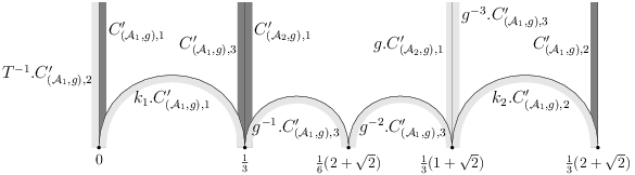
We remark that cyl⁡(𝒜2)=1\cyl(\mathcal{A}_{2})=1. We choose 𝕊={(𝒜1,g),(𝒜2,g)}\mathbb{S}=\{(\mathcal{A}_{1},g),(\mathcal{A}_{2},g)\} and 𝕋:(𝒜1,g)↦0\mathbb{T}\colon(\mathcal{A}_{1},g)\mapsto 0. Figure 3 indicates the induced set of representatives for the cross section.

2.4. The induced discrete dynamical system (D,F)(D,F)

Let

Σ\displaystyle\Sigma :={((𝒜,h),j)|(𝒜,h)∈𝕊, 𝒜 rectangle, j=1,…,cyl⁡(𝒜)}\displaystyle\mathrel{\mathop{:}}=\left\{\big((\mathcal{A},h),j\big)\left|\ \text{$(\mathcal{A},h)\in\mathbb{S}$, $\mathcal{A}$ rectangle, $j=1,\ldots,\cyl(\mathcal{A})$}\vphantom{\big((\mathcal{A},h),j\big)}\right.\right\}
∪{((𝒜,h),j)|(𝒜,h)∈𝕊, 𝒜 triangle, j=1,2,3}\displaystyle\qquad\cup\left\{\big((\mathcal{A},h),j\big)\left|\ \text{$(\mathcal{A},h)\in\mathbb{S}$, $\mathcal{A}$ triangle, $j=1,2,3$}\vphantom{\big((\mathcal{A},h),j\big)}\right.\right\}

denote the arising set of symbols. Then

C′=∐α∈ΣCα′.C^{\prime}=\coprod_{\alpha\in\Sigma}C^{\prime}_{\alpha}.

We call the sets Cα′C^{\prime}_{\alpha}, α∈Σ\alpha\in\Sigma, the components of C′C^{\prime}.

To simplify notations, we use the following conventions. For r∈ℝr\in\mathbb{R} and ε∈{±1}\varepsilon\in\{\pm 1\} we let

⟨r,ε​∞⟩:={(r,∞)if ε=+1(−∞,r)if ε=−1.\langle r,\varepsilon\infty\rangle\mathrel{\mathop{:}}=\begin{cases}(r,\infty)&\text{if $\varepsilon=+1$}\\ (-\infty,r)&\text{if $\varepsilon=-1$.}\end{cases}

Let α∈Σ\alpha\in\Sigma. Recall that Cα′C^{\prime}_{\alpha} is based on the complete geodesic segment (rα,∞)(r_{\alpha},\infty) for a cuspidal point rα∈ℝr_{\alpha}\in\mathbb{R}. We define

εα:={+1if the elements of Cα′ point into {Rez>rα},−1if the elements of Cα′ point into {Rez<rα}.\varepsilon_{\alpha}\mathrel{\mathop{:}}=\begin{cases}+1&\text{if the elements of $C^{\prime}_{\alpha}$ point into $\{\Rea z>r_{\alpha}\}$},\\ -1&\text{if the elements of $C^{\prime}_{\alpha}$ point into $\{\Rea z<r_{\alpha}\}$}.\end{cases}

Further, we let

Iα:=⟨rα,εα∞⟩andDα:=Iα×{α}.I_{\alpha}\mathrel{\mathop{:}}=\langle r_{\alpha},\varepsilon_{\alpha}\infty\rangle\quad\text{and}\quad D_{\alpha}\mathrel{\mathop{:}}=I_{\alpha}\times\{\alpha\}.

Then we have

D=∐α∈ΣDα.D=\coprod_{\alpha\in\Sigma}D_{\alpha}.

An explicit expression for the map F:D→DF\colon D\to D can be deduced as follows. Given a point (r,α)∈Dα(r,\alpha)\in D_{\alpha} for some α∈Σ\alpha\in\Sigma we pick any element v∈Cα′v\in C^{\prime}_{\alpha} such that γv​(∞)=r\gamma_{v}(\infty)=r. Let γ^v=Γ.γv\widehat{\gamma}_{v}=\Gamma.\gamma_{v} be the corresponding geodesic on Γ\ℍ\Gamma\backslash\mathbb{H} and let t0t_{0} be the first return time of γ^v\widehat{\gamma}_{v} to C^\widehat{C}. Then γv′​(t0)\gamma^{\prime}_{v}(t_{0}) is contained in a (unique) Γ\Gamma-translate of some component of C′C^{\prime}, say γv′​(t0)∈g.Cβ′\gamma^{\prime}_{v}(t_{0})\in g.C^{\prime}_{\beta}. Thus,

F(r,α)=(g−1.r,β).F(r,\alpha)=(g^{-1}.r,\beta).

The exact values for gg and β\beta can be algorithmically calculated from the side-pairing in 𝔸\mathbb{A}. The outcome is that FF restricts to a finite number of local diffeomorphisms of the form

(Iα∩g.Iβ)×{α}→Iβ×{β},(r,α)↦(g−1.r,β).\big(I_{\alpha}\cap g.I_{\beta}\big)\times\{\alpha\}\to I_{\beta}\times\{\beta\},\quad(r,\alpha)\mapsto(g^{-1}.r,\beta).

For details we refer to [Poh10].

Example 2.3.

For the lattice Γ\Gamma in Example 2.2 with the choices of 𝔸\mathbb{A}, 𝕊\mathbb{S} and 𝕋\mathbb{T} done there, we have

Σ={((𝒜1,g),1),((𝒜1,g),2),((𝒜1,g),3),((𝒜2,g),1)}.\Sigma=\big\{\left((\mathcal{A}_{1},g),1\right),\left((\mathcal{A}_{1},g),2\right),\left((\mathcal{A}_{1},g),3\right),\left((\mathcal{A}_{2},g),1\right)\big\}.

Moreover, we have

D(𝒜1,g),1\displaystyle D_{(\mathcal{A}_{1},g),1} =(0,∞)×{((𝒜1,g),1)},\displaystyle=(0,\infty)\times\big\{\left((\mathcal{A}_{1},g),1\right)\big\},
D(𝒜1,g),2\displaystyle D_{(\mathcal{A}_{1},g),2} =(−∞,13​(2+2))×{((𝒜1,g),2)},\displaystyle=\left(-\infty,\tfrac{1}{3}(2+\sqrt{2})\right)\times\big\{\left((\mathcal{A}_{1},g),2\right)\big\},
D(𝒜1,g),3\displaystyle D_{(\mathcal{A}_{1},g),3} =(−∞,13)×{((𝒜1,g),3)},\displaystyle=\left(-\infty,\tfrac{1}{3}\right)\times\big\{\left((\mathcal{A}_{1},g),3\right)\big\},
D(𝒜2,g),1\displaystyle D_{(\mathcal{A}_{2},g),1} =(13,∞)×{((𝒜2,g),1)}.\displaystyle=\left(\tfrac{1}{3},\infty\right)\times\big\{\left((\mathcal{A}_{2},g),1\right)\big\}.

The local diffeomorphisms which define the induced discrete dynamical system (D,F)(D,F) can easily be read off from Figure 3, where

k1:=g−1T=(1031)andk2:=gT−1=(1+2−2−43​23−3−2).k_{1}\mathrel{\mathop{:}}=g^{-1}T=\begin{pmatrix}1&0\\ 3&1\end{pmatrix}\quad\text{and}\quad k_{2}\mathrel{\mathop{:}}=gT^{-1}=\begin{pmatrix}1+\sqrt{2}&-2-\frac{4}{3}\sqrt{2}\\ 3&-3-\sqrt{2}\end{pmatrix}.

For example, we have

(0,13)×{((𝒜1,g),1)}→D(𝒜1,g),1,(r,((𝒜1,g),1))↦(k1−1.r,((𝒜1,g),1))\left(0,\tfrac{1}{3}\right)\times\left\{\left((\mathcal{A}_{1},g),1\right)\right\}\to D_{(\mathcal{A}_{1},g),1},\quad\big(r,((\mathcal{A}_{1},g),1)\big)\mapsto\big(k_{1}^{-1}.r,((\mathcal{A}_{1},g),1)\big)

and

(13,∞)×{((𝒜1,g),1)}→D(𝒜2,g),1,(r,((𝒜1,g),1))↦(r,((𝒜2,g),1)).\left(\tfrac{1}{3},\infty\right)\times\left\{\left((\mathcal{A}_{1},g),1\right)\right\}\to D_{(\mathcal{A}_{2},g),1},\quad\big(r,((\mathcal{A}_{1},g),1)\big)\mapsto\big(r,((\mathcal{A}_{2},g),1)\big).
Refer to caption
Figure 3. Set of representatives for cross section (gray) and forward intersections (light gray)

2.5. The associated family of transfer operators

For each s∈ℂs\in\mathbb{C}, the transfer operator with parameter ss associated to the discrete dynamical system (D,F)(D,F) is the operator

(ℒF,s​f)​(x):=∑y∈F−1​(x)f⁡(y)|F′​(y)|s\left(\mathcal{L}_{F,s}f\right)(x)\mathrel{\mathop{:}}=\sum_{y\in F^{-1}(x)}\frac{f(y)}{|F^{\prime}(y)|^{s}}

defined on the space Fct⁡(D,ℂ)\Fct(D;\mathbb{C}) of complex-valued functions on DD. In this section we provide a matrix representation for ℒF,s\mathcal{L}_{F,s}.

For any function φ:V→ℝ\varphi\colon V\to\mathbb{R} on some subset VV of ℝ\mathbb{R} and for any g∈PSL2⁡(ℝ)g\in\PSL_{2}(\mathbb{R}) we set

(3) (τs(g−1)φ)(r):=(g′(r))sφ(g.r)\big(\tau_{s}(g^{-1})\varphi\big)(r)\mathrel{\mathop{:}}=\big(g^{\prime}(r)\big)^{s}\varphi(g.r)

whenever it is well-defined. For appropriate sets VV, the map τs\tau_{s} is a left action of PSL2⁡(ℝ)\PSL_{2}(\mathbb{R}) or Γ\Gamma. It is essentially (depending on conventions) the left-action variant of the so-called slash action.

For α∈Σ\alpha\in\Sigma and f∈Fct⁡(D,ℂ)f\in\Fct(D;\mathbb{C}) we let

fα:=f⋅1Dα,f_{\alpha}\mathrel{\mathop{:}}=f\cdot 1_{D_{\alpha}},

where 1Dα1_{D_{\alpha}} denotes the characteristic function of the set DαD_{\alpha}. Then f=∑α∈Σfαf=\sum_{\alpha\in\Sigma}f_{\alpha}. We may identify ff with the vector (fα)α∈Σ(f_{\alpha})_{\alpha\in\Sigma} and then DαD_{\alpha} with IαI_{\alpha}. Let

(f~α)=f~:=ℒF,s​f.(\widetilde{f}_{\alpha})=\widetilde{f}\mathrel{\mathop{:}}=\mathcal{L}_{F,s}f.

We derive explicit expressions for f~α\widetilde{f}_{\alpha}, α∈Σ\alpha\in\Sigma, in dependence of the component functions fβf_{\beta}, β∈Σ\beta\in\Sigma.

Let α∈Σ\alpha\in\Sigma. Let v∈Cα′v\in C^{\prime}_{\alpha} and suppose that

γv′​((,,,))∩Γ.C′≠∅.\gamma^{\prime}_{v}((-\infty,0))\cap\Gamma.C^{\prime}\not=\emptyset.

Then there exists a previous time of intersection, namely

t1:=max{t<0∣γv′(t)∈Γ.C′}.t_{1}\mathrel{\mathop{:}}=\max\{t<0\mid\gamma^{\prime}_{v}(t)\in\Gamma.C^{\prime}\}.

We call γv′​(t1)\gamma^{\prime}_{v}(t_{1}) the previous intersection of vv. To determine for a given x=(r,α)∈Dαx=(r,\alpha)\in D_{\alpha} its preimages under FF is equivalent to determine for the vectors in Cα′C^{\prime}_{\alpha} their locations of previous intersection. These can be deduced from the side-pairing in 𝔸\mathbb{A} as explained in the following. For Cα′C^{\prime}_{\alpha}, there exists a unique generator (𝒜,h)∈𝕊(\mathcal{A},h)\in\mathbb{S} and a unique element (𝒜′,h′)(\mathcal{A}^{\prime},h^{\prime}) in the cycle determined by (𝒜,h)(\mathcal{A},h) and a unique n∈ℤn\in\mathbb{Z} such that one of the vertical sides of Tn​𝒜′T^{n}\mathcal{A}^{\prime} is contained in the base set of Cα′C^{\prime}_{\alpha} and

Tn​𝒜′⊆{z∈ℍ∣εα⋅(Re⁡z−rα)<0}.T^{n}\mathcal{A}^{\prime}\subseteq\{z\in\mathbb{H}\mid\varepsilon_{\alpha}\cdot(\Rea z-r_{\alpha})<0\}.

In other words, some subset of Cα′C^{\prime}_{\alpha} is based on a vertical side of Tn​𝒜′T^{n}\mathcal{A}^{\prime} and the elements of Cα′C^{\prime}_{\alpha} do not point into Tn​𝒜′T^{n}\mathcal{A}^{\prime}. In this case, we say that Cα′C^{\prime}_{\alpha} is neighboring Tn​𝒜′T^{n}\mathcal{A}^{\prime}. We have to distinguish the following three situations:

Situation (1): 𝒜′\mathcal{A}^{\prime} is a rectangle. Then we are in one of the situations shown in Figure 4.

Refer to caption
Figure 4. Situation (1)

Situation (2): 𝒜′\mathcal{A}^{\prime} is a triangle and Cα′C^{\prime}_{\alpha} is neighboring Tn​𝒜′T^{n}\mathcal{A}^{\prime} on its long side. Then we are in one of the situations shown in Figure 5.

Refer to caption
Figure 5. Situation (2)

Situation (3): 𝒜′\mathcal{A}^{\prime} is a triangle and Cα′C^{\prime}_{\alpha} is neighboring Tn​𝒜′T^{n}\mathcal{A}^{\prime} on its short side. Then we are in one of the situations shown in Figure 6.

Refer to caption
Figure 6. Situation (3)

Note that the two sub-situations shown in any of the Figures 4-6 are mirror-inverted and thus are equivalent for all further considerations. We will not distinguish these in the following figures. However, their differences are taken into account in all formulas by εα\varepsilon_{\alpha}. For the locations of the previous intersections we have to subdivide these situations. All further numbering of situations will refer to and extend the ones just introduced.

Situation (1): Let ((𝒜ℓ,hℓ))ℓ=1,…,k\big((\mathcal{A}_{\ell},h_{\ell})\big)_{\ell=1,\ldots,k} be the cycle determined by (𝒜,h)(\mathcal{A},h) and suppose that 𝒜′=𝒜j\mathcal{A}^{\prime}=\mathcal{A}_{j} for some j∈{1,…,k}j\in\{1,\ldots,k\}. We set

C′ℓ:=C′(𝒜,h),ℓ,fℓ:=f(𝒜,h),ℓandεℓ:=ε(𝒜,h),ℓC^{\prime}_{\ell}\mathrel{\mathop{:}}=C^{\prime}_{(\mathcal{A},h),\ell},\quad f_{\ell}\mathrel{\mathop{:}}=f_{(\mathcal{A},h),\ell}\quad\text{and}\quad\varepsilon_{\ell}\mathrel{\mathop{:}}=\varepsilon_{(\mathcal{A},h),\ell}

for ℓ=1,…,k\ell=1,\ldots,k, where the index ℓ\ell is understood modulo cyl⁡(𝒜)\cyl(\mathcal{A}). According to the rotation direction of the cycle related to the orientation of Cα′C^{\prime}_{\alpha} we are either in Situation (1a) shown in Figure 7 (εα=εj\varepsilon_{\alpha}=\varepsilon_{j}) or in Situation (1b) shown in Figure 8 (εα=−εj\varepsilon_{\alpha}=-\varepsilon_{j}).

Refer to caption
Figure 7. Situation (1a)
Refer to caption
Figure 8. Situation (1b)

In Situation (1a) we have

f~α\displaystyle\widetilde{f}_{\alpha} =τs​(Tn)​fj+τs​(Tn​hj−1)​fj+1+⋯+τs​(Tn​hj−1​…​hj+k−3−1)​fj+k−2\displaystyle=\tau_{s}(T^{n})f_{j}+\tau_{s}(T^{n}h_{j}^{-1})f_{j+1}+\cdots+\tau_{s}(T^{n}h_{j}^{-1}\ldots h_{j+k-3}^{-1})f_{j+k-2}
=∑ℓ=0k−2τs(Tnhj−1⋯hj+ℓ−1−1)fj+ℓ,\displaystyle=\sum_{\ell=0}^{k-2}\tau_{s}(T^{n}h_{j}^{-1}\cdots h_{j+\ell-1}^{-1})f_{j+\ell},

whereas in Situation (1b) we have

f~α\displaystyle\widetilde{f}_{\alpha} =τs​(Tn​hj−1)​fj+1+τs​(Tn​hj−1​hj+1−1)​fj+2+⋯+τs​(Tn​hj−1​…​hj+k−2−1)​fj+k−1\displaystyle=\tau_{s}(T^{n}h_{j}^{-1})f_{j+1}+\tau_{s}(T^{n}h_{j}^{-1}h_{j+1}^{-1})f_{j+2}+\cdots+\tau_{s}(T^{n}h_{j}^{-1}\ldots h_{j+k-2}^{-1})f_{j+k-1}
=∑ℓ=0k−2τs(Tnhj−1⋯hj+ℓ−1)fj+ℓ+1.\displaystyle=\sum_{\ell=0}^{k-2}\tau_{s}(T^{n}h_{j}^{-1}\cdots h_{j+\ell}^{-1})f_{j+\ell+1}.

Situation (2): Let ((𝒜,h),(𝒜′,h−1))\big((\mathcal{A},h),(\mathcal{A}^{\prime},h^{-1})\big) be the cycle determined by (𝒜,h)(\mathcal{A},h) (note that this 𝒜′\mathcal{A}^{\prime} is not necessarily the 𝒜′\mathcal{A}^{\prime} from above) and let m:=m⁡(𝒜,h)m\mathrel{\mathop{:}}=m(\mathcal{A},h). We set Cj′:=C(𝒜,h),j′C^{\prime}_{j}\mathrel{\mathop{:}}=C^{\prime}_{(\mathcal{A},h),j}, fj:=f(𝒜,h),jf_{j}\mathrel{\mathop{:}}=f_{(\mathcal{A},h),j} and εj:=ε(𝒜,h),j\varepsilon_{j}\mathrel{\mathop{:}}=\varepsilon_{(\mathcal{A},h),j} for j=1,2,3j=1,2,3. Then we have either Situation (2a) (εα=ε1\varepsilon_{\alpha}=\varepsilon_{1}) or Situation (2b) (εα=−ε1\varepsilon_{\alpha}=-\varepsilon_{1}) shown in Figure 9.

Refer to caption
Figure 9. On the left Situation (2a), on the right Situation (2b)

In Situation (2a) we have

f~α=τs​(Tn​h)​f1+τs​(Tn​h​T−m)​f3,\widetilde{f}_{\alpha}=\tau_{s}(T^{n}h)f_{1}+\tau_{s}(T^{n}hT^{-m})f_{3},

and in Situation (2b) we have

f~α=τs​(Tn​h−1)​f2+τs​(Tn−m)​f3.\widetilde{f}_{\alpha}=\tau_{s}(T^{n}h^{-1})f_{2}+\tau_{s}(T^{n-m})f_{3}.

Situation (3): We use the notation from Situation (2). Then we have either Situation (3a) (εα=ε1\varepsilon_{\alpha}=\varepsilon_{1}) or Situation (3b) (εα=−ε1\varepsilon_{\alpha}=-\varepsilon_{1}) shown in Figure 10.

Refer to caption
Figure 10. On the left Situation (3a), on the right Situation (3b)

In Situation (3a) we have

f~α=τs​(Tn)​f1+τs​(Tn​h−1)​f2,\widetilde{f}_{\alpha}=\tau_{s}(T^{n})f_{1}+\tau_{s}(T^{n}h^{-1})f_{2},

whereas in Situation (3b) we have

f~α=τs​(Tn​h)​f1+τs​(Tn)​f2.\widetilde{f}_{\alpha}=\tau_{s}(T^{n}h)f_{1}+\tau_{s}(T^{n})f_{2}.
Example 2.4.

Continuing Example 2.3, we deduce the associated family of transfer operators. The locations of previous intersections can easily be read off from Figure 11.

Refer to caption
Figure 11. Set of representatives for cross section (gray) and backward intersections (light gray)

Using the identification

f=(f(𝒜1,g),1f(𝒜1,g),2f(𝒜1,g),3f(𝒜2,g),1)f=\begin{pmatrix}f_{(\mathcal{A}_{1},g),1}\\ f_{(\mathcal{A}_{1},g),2}\\ f_{(\mathcal{A}_{1},g),3}\\ f_{(\mathcal{A}_{2},g),1}\end{pmatrix}

(in this order), the associated transfer operator ℒs\mathcal{L}_{s} with parameter ss is represented by the matrix

ℒs=(τs​(k1−1)0τs​(k1−1)00τs​(k2−1)τs​(T)0000τs​(g)+τs​(g2)+τs​(g3)1τs​(g−1)00).\mathcal{L}_{s}=\begin{pmatrix}\tau_{s}(k_{1}^{-1})&0&\tau_{s}(k_{1}^{-1})&0\\ 0&\tau_{s}(k_{2}^{-1})&\tau_{s}(T)&0\\ 0&0&0&\tau_{s}(g)+\tau_{s}(g^{2})+\tau_{s}(g^{3})\\ 1&\tau_{s}(g^{-1})&0&0\end{pmatrix}.

2.6. Period functions

Let s∈ℂs\in\mathbb{C}. We say that a function φ:ℝ→ℂ\varphi\colon\mathbb{R}\to\mathbb{C} extends smoothly (C∞C^{\infty}) to P1​(ℝ)P^{1}(\mathbb{R}) if for some (and indeed any) element g∈PSL2⁡(ℝ)g\in\PSL_{2}(\mathbb{R}), g.∞≠∞g.\infty\not=\infty, the functions φ\varphi and τs​(g)​φ\tau_{s}(g)\varphi are smooth on ℝ\mathbb{R}. Note that this notion of smooth extension depends on ss.

For any α∈Σ\alpha\in\Sigma, we find a unique β∈Σ\beta\in\Sigma and unique g∈Γg\in\Gamma such that Cα′C^{\prime}_{\alpha} and g.Cβ′g.C^{\prime}_{\beta} are based on the same geodesic segment but are disjoint. We call (β,g)(\beta,g) the tuple assigned to α\alpha. The precise values for β\beta and gg can be read off from Situations (1a)–(3b). For f∈Fct⁡(D,ℂ)f\in\Fct(D;\mathbb{C}) we define

(4) ψα,f:={εα​fαon ⟨rα,εα​∞⟩−εα​τs​(g)​fβon ⟨rα,−εα​∞⟩.\psi_{\alpha,f}\mathrel{\mathop{:}}=\begin{cases}\varepsilon_{\alpha}f_{\alpha}&\text{on $\langle r_{\alpha},\varepsilon_{\alpha}\infty\rangle$}\\ -\varepsilon_{\alpha}\tau_{s}(g)f_{\beta}&\text{on $\langle r_{\alpha},-\varepsilon_{\alpha}\infty\rangle$.}\end{cases}

The space of period functions FEsω,dec⁡(Γ,𝔸,𝕊,𝕋)\FE_{s}^{\omega,\text{dec}}(\Gamma;\mathbb{A},\mathbb{S},\mathbb{T}) (relative to the choices of 𝔸\mathbb{A}, 𝕊\mathbb{S} and 𝕋\mathbb{T}) is defined to be the space of function vectors

f=(fα)α∈Σf=(f_{\alpha})_{\alpha\in\Sigma}

such that

  • (PF1)

    fα∈Cω​(Iα,ℂ)f_{\alpha}\in C^{\omega}(I_{\alpha};\mathbb{C}) for α∈Σ\alpha\in\Sigma,

  • (PF2)

    f=ℒF,s​ff=\mathcal{L}_{F,s}f.

  • (PF3)

    If for α∈Σ\alpha\in\Sigma, the map ψα,f\psi_{\alpha,f} in (4) arises from Situation (1a) or (3b) (that is, β\beta and gg are determined by these situations), then ψα,f\psi_{\alpha,f} extends smoothly to ℝ\mathbb{R}.

  • (PF4)

    If for α∈Σ\alpha\in\Sigma, the map ψα,f\psi_{\alpha,f} is not determined by Situation (1a) or (3b), then it extends smoothly to P1​(ℝ)P^{1}(\mathbb{R}).

Remark 2.5.

If (PF3) is satisfied, then the maps considered there actually extend smoothly to P1​(ℝ)P^{1}(\mathbb{R}) by the following argument: If

ψα={εα​fαon ⟨rα,εα​∞⟩−εα​τs​(g)​fβon ⟨rα,−εα​∞⟩\psi_{\alpha}=\begin{cases}\varepsilon_{\alpha}f_{\alpha}&\text{on $\langle r_{\alpha},\varepsilon_{\alpha}\infty\rangle$}\\ -\varepsilon_{\alpha}\tau_{s}(g)f_{\beta}&\text{on $\langle r_{\alpha},-\varepsilon_{\alpha}\infty\rangle$}\end{cases}

is one of these maps, then

ψβ={εβ​fβon ⟨rβ,εβ​∞⟩−εβ​τs​(g−1)​fαon ⟨rβ,−εβ​∞⟩\psi_{\beta}=\begin{cases}\varepsilon_{\beta}f_{\beta}&\text{on $\langle r_{\beta},\varepsilon_{\beta}\infty\rangle$}\\ -\varepsilon_{\beta}\tau_{s}(g^{-1})f_{\alpha}&\text{on $\langle r_{\beta},-\varepsilon_{\beta}\infty\rangle$}\end{cases}

is also one and εα=εβ\varepsilon_{\alpha}=\varepsilon_{\beta}, rβ=g−1.∞r_{\beta}=g^{-1}.\infty and g−1.rα=∞g^{-1}.r_{\alpha}=\infty. Thus, τs​(g−1)​ψα=ψβ\tau_{s}(g^{-1})\psi_{\alpha}=\psi_{\beta}.

Example 2.6.

For the lattice Γ\Gamma from Example 2.2 with the choices of 𝔸\mathbb{A}, 𝕊\mathbb{S} and 𝕋\mathbb{T} done there we set

f1:=f(𝒜1,g),1,f2:=f(𝒜1,g),2,f3:=f(𝒜1,g),3,andf4:=f(𝒜2,g),1.f_{1}\mathrel{\mathop{:}}=f_{(\mathcal{A}_{1},g),1},\ f_{2}\mathrel{\mathop{:}}=f_{(\mathcal{A}_{1},g),2},\ f_{3}\mathrel{\mathop{:}}=f_{(\mathcal{A}_{1},g),3},\ \text{and}\ f_{4}\mathrel{\mathop{:}}=f_{(\mathcal{A}_{2},g),1}.

The space of period functions FEsω,dec⁡(Γ,𝔸,𝕊,𝕋)\FE_{s}^{\omega,\text{dec}}(\Gamma;\mathbb{A},\mathbb{S},\mathbb{T}) consists of the function vectors f=(f1,…,f4)f=(f_{1},\ldots,f_{4}) such that

  1. (i)

    the function f1f_{1} is real-analytic on (0,∞)(0,\infty), the function f2f_{2} is real-analytic on (−∞,13​(2+2))\big(-\infty,\tfrac{1}{3}(2+\sqrt{2})\big), the function f3f_{3} is real-analytic on (−∞,13)\big(-\infty,\tfrac{1}{3}\big), and the function f4f_{4} is real-analytic on (13,∞)\big(\tfrac{1}{3},\infty\big),

  2. (ii)

    the following system of functional equations is satisfied:

    f1\displaystyle f_{1} =τs​(k1−1)​f1+τs​(k1−1)​f3\displaystyle=\tau_{s}(k_{1}^{-1})f_{1}+\tau_{s}(k_{1}^{-1})f_{3}
    f2\displaystyle f_{2} =τs​(k2−1)​f2+τs​(T)​f3\displaystyle=\tau_{s}(k_{2}^{-1})f_{2}+\tau_{s}(T)f_{3}
    f3\displaystyle f_{3} =τs​(g)​f4+τs​(g2)​f4+τs​(g3)​f4\displaystyle=\tau_{s}(g)f_{4}+\tau_{s}(g^{2})f_{4}+\tau_{s}(g^{3})f_{4}
    f4\displaystyle f_{4} =f1+τs​(g−1)​f2,\displaystyle=f_{1}+\tau_{s}(g^{-1})f_{2},
  3. (iii)

    the maps

    {f1on (0,∞)−τs​(T−1)​f2on (−∞,0)and{f4on (13,∞)−f3on (−∞,13)\begin{cases}f_{1}&\text{on $(0,\infty)$}\\ -\tau_{s}(T^{-1})f_{2}&\text{on $(-\infty,0)$}\end{cases}\quad\text{and}\quad\begin{cases}f_{4}&\text{on $\big(\tfrac{1}{3},\infty\big)$}\\ -f_{3}&\text{on $\big(-\infty,\tfrac{1}{3}\big)$}\end{cases}

    extend smoothly to P1​(ℝ)P^{1}(\mathbb{R}).

2.7. Parabolic 11-cohomology

For the proof of Theorem A we take advantage of the characterization in [BLZ12] of Maass cusp forms with eigenvalue s⁡(1−s)s(1-s) as parabolic 11-cocycle classes with values in the semi-analytic smooth vectors of the principal series representation with spectral parameter ss. In the following we briefly recall this characterization.

Let s∈ℂs\in\mathbb{C}. The space 𝒱sω∗,∞\mathcal{V}_{s}^{\omega*,\infty} of semi-analytic smooth vectors in the line model of the principal series representation with spectral parameter ss is the space of functions φ:ℝ→ℂ\varphi\colon\mathbb{R}\to\mathbb{C} which are smooth and extend smoothly to P1​(ℝ)P^{1}(\mathbb{R}) and are real-analytic on ℝ∖E\mathbb{R}\smallsetminus E, where EE is a finite subset which may depend on φ\varphi. The lattice Γ\Gamma acts on 𝒱sω∗,∞\mathcal{V}_{s}^{\omega*,\infty} via the action τs\tau_{s} from (3).

Recall that the space of 11-cocycles of group cohomology of Γ\Gamma with values in 𝒱sω∗,∞\mathcal{V}_{s}^{\omega*,\infty} is

Z1(Γ;𝒱sω∗,∞)={c:Γ→𝒱sω∗,∞∣∀g,h∈Γ:cg​h=τs(h−1)cg+ch}.Z^{1}(\Gamma;\mathcal{V}_{s}^{\omega*,\infty})=\{c\colon\Gamma\to\mathcal{V}_{s}^{\omega*,\infty}\mid\forall\,g,h\in\Gamma\colon c_{gh}=\tau_{s}(h^{-1})c_{g}+c_{h}\}.

We use here the notation of restricted cocycles and write cg∈𝒱sω∗,∞c_{g}\in\mathcal{V}_{s}^{\omega*,\infty} for the image c⁡(g)c(g) of g∈Γg\in\Gamma under c:Γ→𝒱sω∗,∞c\colon\Gamma\to\mathcal{V}_{s}^{\omega*,\infty}. The space of parabolic 11-cocycles is

Zpar1(Γ;𝒱sω∗,∞)={c∈Z1(Γ;𝒱sω∗,∞)|∀p∈Γparabolic∃ψ∈𝒱sω∗,∞:cp=τs​(p−1)​ψ−ψ}.Z^{1}_{\text{par}}(\Gamma;\mathcal{V}_{s}^{\omega*,\infty})=\left\{c\in Z^{1}(\Gamma;\mathcal{V}_{s}^{\omega*,\infty})\left|\ \begin{split}&\forall\,p\in\Gamma\ \text{parabolic}\ \exists\,\psi\in\mathcal{V}_{s}^{\omega*,\infty}\colon\\ &c_{p}=\tau_{s}(p^{-1})\psi-\psi\end{split}\right.\right\}.

The spaces of 11-coboundaries of group cohomology and of parabolic cohomology are equal. They are

Bpar1(Γ;𝒱sω∗,∞)=B1(Γ;𝒱sω∗,∞)={g↦τs(g−1)ψ−ψ∣ψ∈𝒱sω∗,∞}.B^{1}_{\text{par}}(\Gamma;\mathcal{V}_{s}^{\omega*,\infty})=B^{1}(\Gamma;\mathcal{V}_{s}^{\omega*,\infty})=\{g\mapsto\tau_{s}(g^{-1})\psi-\psi\mid\psi\in\mathcal{V}_{s}^{\omega*,\infty}\}.

Then the parabolic 11-cohomology space is the quotient space

Hpar1(Γ;𝒱sω∗,∞)=Zpar1(Γ;𝒱sω∗,∞)/Bpar1(Γ;𝒱sω∗,∞).H^{1}_{\text{par}}(\Gamma;\mathcal{V}_{s}^{\omega*,\infty})=Z^{1}_{\text{par}}(\Gamma;\mathcal{V}_{s}^{\omega*,\infty})/B^{1}_{\text{par}}(\Gamma;\mathcal{V}_{s}^{\omega*,\infty}).

Let MCFs⁡(Γ)\MCF_{s}(\Gamma) denote the space of Maass cusp forms for Γ\Gamma with eigenvalue s⁡(1−s)s(1-s).

Theorem 2.7 ([BLZ12]).

Let s∈ℂs\in\mathbb{C} with Re⁡s∈(0,1)\Rea s\in(0,1). Then the vector spaces MCFs⁡(Γ)\MCF_{s}(\Gamma) and Hpar1(Γ;𝒱sω∗,∞)H^{1}_{\text{par}}(\Gamma;\mathcal{V}_{s}^{\omega*,\infty}) are isomorphic.

The isomorphism in Theorem 2.7 is constructive and given by the following integral transform. Let u∈MCFs⁡(Γ)u\in\MCF_{s}(\Gamma) and choose any z0∈ℍz_{0}\in\mathbb{H} or cuspidal. Then the parabolic 11-cocycle class [c]∈Hpar1(Γ;𝒱sω∗,∞)[c]\in H^{1}_{\text{par}}(\Gamma;\mathcal{V}_{s}^{\omega*,\infty}) associated to uu is represented by the cocycle cc given by

cg​(r):=∫g−1.z0z0[u,R​(r,⋅)s]c_{g}(r)\mathrel{\mathop{:}}=\int_{g^{-1}.z_{0}}^{z_{0}}[u,R(r,\cdot)^{s}]

for g∈Γg\in\Gamma. Here we use R:ℝ×ℍ→ℍR\colon\mathbb{R}\times\mathbb{H}\to\mathbb{H},

R⁡(r,z):=Im⁡(1r−z)R(r,z)\mathrel{\mathop{:}}=\Ima\left(\frac{1}{r-z}\right)

and

[u,v]:=∂u∂z⋅v⋅dz+u⋅∂v∂z¯⋅dz¯(Green form)[u,v]\mathrel{\mathop{:}}=\frac{\partial u}{\partial z}\cdot v\cdot dz+u\cdot\frac{\partial v}{\partial\overline{z}}\cdot d\overline{z}\qquad\text{(Green form)}

for any complex-valued smooth function vv on ℍ\mathbb{H}. The integration is performed along any differentiable path from g−1.z0g^{-1}.z_{0} to z0z_{0} which is essentially contained in ℍ\mathbb{H}. The integral is well-defined since the 11-form [u,R​(r,⋅)s][u,R(r,\cdot)^{s}] is closed. A change of the choice of z0z_{0} changes cc by a parabolic 11-coboundary. The Γ\Gamma-action via τs\tau_{s} translates into a change of path of integration. More precisely, we have

(5) τs​(g−1)​∫ab[u,R​(r,⋅)s]=∫g−1.ag−1.b[u,R​(r,⋅)s]\tau_{s}(g^{-1})\int_{a}^{b}[u,R(r,\cdot)^{s}]=\int_{g^{-1}.a}^{g^{-1}.b}[u,R(r,\cdot)^{s}]

for all g∈Γg\in\Gamma and cuspidal points a,ba,b.

3. Isomorphism of period functions and Maass cusp forms

In this section we prove the following statement:

Theorem 3.1.

For s∈ℂs\in\mathbb{C} with Re⁡s∈(0,1)\Rea s\in(0,1), the vector spaces FEsω,dec⁡(Γ,𝔸,𝕊,𝕋)\FE_{s}^{\omega,\text{dec}}(\Gamma;\mathbb{A},\mathbb{S},\mathbb{T}) and Hpar1(Γ;𝒱sω∗,∞)H^{1}_{\text{par}}(\Gamma;\mathcal{V}_{s}^{\omega*,\infty}) are isomorphic.

This, together with Theorem 2.7, establishes Theorem A. The isomorphism in Theorem 3.1 is provided by the two constructions presented in the following. For these, let

Σ′:={α∈Σ∣rα is Γ-equivalent to ∞}.\Sigma^{\prime}\mathrel{\mathop{:}}=\{\alpha\in\Sigma\mid\text{$r_{\alpha}$ is $\Gamma$-equivalent to $\infty$}\}.

If α∈Σ′\alpha\in\Sigma^{\prime}, then Cα′C^{\prime}_{\alpha} is as in Situation (1) or (3). Hence there exists b∈Γb\in\Gamma such that Cα′C^{\prime}_{\alpha} is based on the geodesic segment (b−1.∞,∞)(b^{-1}.\infty,\infty). The element bb is unique only up to left multiplication with elements in Γ∞\Gamma_{\infty}. Let (β,g)(\beta,g) be the tuple assigned to α\alpha (cf. Section 2.6). For any possible choice of bb, we call (β,g,b)(\beta,g,b) a triple assigned to α\alpha. Let

𝒮:={b∈Γ∣∃α∈Σ′​∃β∈Σ​∃g∈Γ:(β,g,b) is assigned to α}∪{T}.\mathcal{S}\mathrel{\mathop{:}}=\{b\in\Gamma\mid\text{$\exists\,\alpha\in\Sigma^{\prime}\ \exists\,\beta\in\Sigma\ \exists\,g\in\Gamma\colon(\beta,g,b)$ is assigned to $\alpha$}\}\cup\{T\}.
  1. (a)

    Let f∈FEsω,dec⁡(Γ,𝔸,𝕊,𝕋)f\in\FE_{s}^{\omega,\text{dec}}(\Gamma;\mathbb{A},\mathbb{S},\mathbb{T}). We define a map

    c:=c(f):𝒮→𝒱sω∗,∞c\mathrel{\mathop{:}}=c(f)\colon\mathcal{S}\to\mathcal{V}^{\omega*,\infty}_{s}

    by cT:=0c_{T}\mathrel{\mathop{:}}=0 and

    cb:=ψα,ffor α∈Σ′,c_{b}\mathrel{\mathop{:}}=\psi_{\alpha,f}\quad\text{for $\alpha\in\Sigma^{\prime}$,}

    where (β,g,b)∈Σ×Γ×Γ(\beta,g,b)\in\Sigma\times\Gamma\times\Gamma is a triple assigned to α\alpha. Proposition 3.3 below shows that cc determines a unique parabolic 11-cocycle.

  2. (b)

    Let [c]∈Hpar1(Γ;𝒱sω∗,∞)[c]\in H^{1}_{\text{par}}(\Gamma;\mathcal{V}_{s}^{\omega*,\infty}). Pick its unique representative c∈Zpar1(Γ;𝒱sω∗,∞)c\in Z^{1}_{\text{par}}(\Gamma;\mathcal{V}_{s}^{\omega*,\infty}) for which cT=0c_{T}=0. We associate to [c][c] a function vector f⁡([c])=(fα)α∈Σf([c])=(f_{\alpha})_{\alpha\in\Sigma} as follows. Suppose first that α∈Σ′\alpha\in\Sigma^{\prime}. Pick a triple (β,g,b)∈Σ×Γ×Γ(\beta,g,b)\in\Sigma\times\Gamma\times\Gamma which is assigned to α\alpha. We define

    fα:=εα​cb⋅1Iα.f_{\alpha}\mathrel{\mathop{:}}=\varepsilon_{\alpha}c_{b}\cdot 1_{I_{\alpha}}.

    Suppose now that α∈Σ∖Σ′\alpha\in\Sigma\smallsetminus\Sigma^{\prime}. Recall that Cα′C^{\prime}_{\alpha} is then based on a geodesic segment of the form (v,∞)(v,\infty) with vv being a cuspidal point which is not Γ\Gamma-equivalent to ∞\infty. Let pp be a generator of StabΓ⁡(v)\Stab_{\Gamma}(v). Let ψ∈𝒱sω∗,∞\psi\in\mathcal{V}_{s}^{\omega*,\infty} be the unique element (see [Poh12, Lemma 3.3]) such that

    cp=τs​(p−1)​ψ−ψ.c_{p}=\tau_{s}(p^{-1})\psi-\psi.

    We define

    fα:=−εαψ⋅1Iα.f_{\alpha}\mathrel{\mathop{:}}=-\varepsilon_{\alpha}\psi\cdot 1_{I_{\alpha}}.

Instead of Theorem 3.1 we show its following concretization.

Theorem 3.2.

Let s∈ℂs\in\mathbb{C} with 0<Re⁡s<10<\Rea s<1. Then the map

FEsω,dec(Γ;𝔸,𝕊,𝕋)→Hpar1(Γ;𝒱sω∗,∞),f↦[c(f)]\FE_{s}^{\omega,\text{dec}}(\Gamma;\mathbb{A},\mathbb{S},\mathbb{T})\to H^{1}_{\text{par}}(\Gamma;\mathcal{V}_{s}^{\omega*,\infty}),\quad f\mapsto[c(f)]

is a linear isomorphism. Its inverse map is given by

Hpar1(Γ;𝒱sω∗,∞)→FEsω,dec(Γ;𝔸,𝕊,𝕋),[c]↦f([c]).H^{1}_{\text{par}}(\Gamma;\mathcal{V}_{s}^{\omega*,\infty})\to\FE_{s}^{\omega,\text{dec}}(\Gamma;\mathbb{A},\mathbb{S},\mathbb{T}),\quad[c]\mapsto f([c]).

The proof of Theorem 3.2 is split into Propositions 3.3 and 3.5 below.

Proposition 3.3.

If f∈FEsω,dec⁡(Γ,𝔸,𝕊,𝕋)f\in\FE_{s}^{\omega,\text{dec}}(\Gamma;\mathbb{A},\mathbb{S},\mathbb{T}), then c⁡(f)c(f) determines a unique element in Zpar1(Γ;𝒱sω∗,∞)Z^{1}_{\text{par}}(\Gamma;\mathcal{V}_{s}^{\omega*,\infty}).

Remark 3.4.

In order to extend c:=c⁡(f)c\mathrel{\mathop{:}}=c(f) to all of Γ\Gamma and to show that this extension is well-defined, unique and a 11-cocycle, we want to apply the Poincaré Fundamental Polyhedron Theorem (see e.g. [Mas71]) to the (closed) fundamental region ⋃𝔸\bigcup\mathbb{A} for Γ\Gamma. The Poincaré Theorem in its usual form however may only be applied if ⋃𝔸\bigcup\mathbb{A} is connected. For each 𝒜∈𝔸\mathcal{A}\in\mathbb{A} we can use an appropriate TT-shift, say Tn⁡(𝒜)T^{n(\mathcal{A})}, such that the union over the family

𝔸′:={Tn⁡(𝒜)​𝒜∣𝒜∈𝔸}\mathbb{A}^{\prime}\mathrel{\mathop{:}}=\{T^{n(\mathcal{A})}\mathcal{A}\mid\mathcal{A}\in\mathbb{A}\}

provides a (connected, closed) fundamental domain for Γ\Gamma. The side-pairing elements of the non-vertical sides of the elements in 𝔸′\mathbb{A}^{\prime} are also TT-shifted compared to the original ones. If we apply the Poincaré Theorem to ⋃𝔸′\bigcup\mathbb{A}^{\prime} to deduce the relations between the side-pairing elements, the TT-shifts will cancel and we will find the same relations as if we had applied the Poincaré Theorem to ⋃𝔸\bigcup\mathbb{A}. In short, for our purposes we may apply the Poincaré Theorem to ⋃𝔸\bigcup\mathbb{A} if we add TT to the set of generators even though it need not be a side-pairing element.

Proof of Proposition 3.3.

Let c:=c⁡(f)c\mathrel{\mathop{:}}=c(f). The Poincaré Theorem shows that Γ\Gamma is generated (as a group) by 𝒮\mathcal{S}. Therefore, using the definition of cc on 𝒮\mathcal{S} we can extend cc to all of Γ\Gamma via the cocycle relation. If this extension (which we also call cc) is well-defined, then it is unique. Moreover, the properties (PF3) and (PF4) in Section 2.6 and Remark 2.5 yield that cc takes values in 𝒱sω∗,∞\mathcal{V}_{s}^{\omega*,\infty}. To show that cc is well-defined and indeed defines a 11-cocycle we proceed in the following steps. The Poincaré Theorem yields that these are sufficient.

  1. (i)

    If b1=Tn​b2b_{1}=T^{n}b_{2} for some b1,b2∈𝒮b_{1},b_{2}\in\mathcal{S}, n∈ℤn\in\mathbb{Z}, then we have to show that

    cb1=τs​(b2−1)​cTn+cb2.c_{b_{1}}=\tau_{s}(b_{2}^{-1})c_{T^{n}}+c_{b_{2}}.

    Now cT=0c_{T}=0 implies cTn=0c_{T^{n}}=0, and by definition cb1=cb2c_{b_{1}}=c_{b_{2}}. Thus, this condition is satisfied. Moreover, we may use cTn​g=cgc_{T^{n}g}=c_{g} in any of the following considerations.

  2. (ii)

    Suppose that we have b,b−1∈𝒮∖{T}b,b^{-1}\in\mathcal{S}\smallsetminus\{T\} (or more general, b,Tn​b−1∈𝒮b,T^{n}b^{-1}\in\mathcal{S}). We need to show τs​(b)​cb=−cb−1\tau_{s}(b)c_{b}=-c_{b^{-1}}. There exist α,β∈Σ′\alpha,\beta\in\Sigma^{\prime} and g∈Γg\in\Gamma such that Cα′,g.Cβ′C^{\prime}_{\alpha},g.C^{\prime}_{\beta} are both based on the geodesic segment (b−1.∞,∞)(b^{-1}.\infty,\infty) but are disjoint. Moreover, b.Cα′,b​g.Cβ′b.C^{\prime}_{\alpha},bg.C^{\prime}_{\beta} are the two translates of some components of C′C^{\prime} which are both based on the geodesic segment (b.∞,∞)(b.\infty,\infty), see Figure 12.

    Refer to caption
    Figure 12. Situation for b,b−1∈𝒮∖{T}b,b^{-1}\in\mathcal{S}\smallsetminus\{T\}

    Thus, b​g=Tnbg=T^{n} for some n∈ℤn\in\mathbb{Z}. Using (i) we may suppose n=0n=0. Then

    cb=ψα,f={εα​fαon ⟨b−1.∞,εα∞⟩−εα​τs​(b−1)​fβon ⟨b−1.∞,−εα∞⟩c_{b}=\psi_{\alpha,f}=\begin{cases}\varepsilon_{\alpha}f_{\alpha}&\text{on $\langle b^{-1}.\infty,\varepsilon_{\alpha}\infty\rangle$}\\ -\varepsilon_{\alpha}\tau_{s}(b^{-1})f_{\beta}&\text{on $\langle b^{-1}.\infty,-\varepsilon_{\alpha}\infty\rangle$}\end{cases}

    and

    cb−1=ψβ,f={εβ​fβon ⟨b.∞,εβ∞⟩−εβ​τs​(b)​fαon ⟨b.∞,−εβ∞⟩.c_{b^{-1}}=\psi_{\beta,f}=\begin{cases}\varepsilon_{\beta}f_{\beta}&\text{on $\langle b.\infty,\varepsilon_{\beta}\infty\rangle$}\\ -\varepsilon_{\beta}\tau_{s}(b)f_{\alpha}&\text{on $\langle b.\infty,-\varepsilon_{\beta}\infty\rangle$.}\end{cases}

    Since εα=εβ=⁣:ε\varepsilon_{\alpha}=\varepsilon_{\beta}\mathrel{=\mkern-4.5mu{\mathop{:}}}\varepsilon it follows

    τs​(b)​cb\displaystyle\tau_{s}(b)c_{b} ={ε​τs​(b)​fαon ⟨b.∞,−ε∞⟩−ε​fβon ⟨b.∞,ε∞⟩\displaystyle=\begin{cases}\varepsilon\tau_{s}(b)f_{\alpha}&\text{on $\langle b.\infty,-\varepsilon\infty\rangle$}\\ -\varepsilon f_{\beta}&\text{on $\langle b.\infty,\varepsilon\infty\rangle$}\end{cases}
    =−cb−1.\displaystyle=-c_{b^{-1}}.
  3. (iii)

    Let (𝒜,h)∈𝕊(\mathcal{A},h)\in\mathbb{S} with 𝒜\mathcal{A} being a rectangle and let ((𝒜j,hj))j=1,…,k\big((\mathcal{A}_{j},h_{j})\big)_{j=1,\ldots,k} be the cycle determined by (𝒜,h)(\mathcal{A},h). We have to show that

    chj+k−1⋯hj+1hj=0c_{h_{j+k-1}\cdots h_{j+1}h_{j}}=0

    for some j∈{1,…,k}j\in\{1,\ldots,k\}, where we understand the indices of the hℓh_{\ell} modulo kk. Let ℓ∈{1,…,k}\ell\in\{1,\ldots,k\}. Then hℓ∈𝒮h_{\ell}\in\mathcal{S}. Let αℓ:=((𝒜,h),ℓ)\alpha_{\ell}\mathrel{\mathop{:}}=\big((\mathcal{A},h),\ell\big) and (βℓ,gℓ)∈Σ×Γ(\beta_{\ell},g_{\ell})\in\Sigma\times\Gamma be the tuple assigned to αℓ\alpha_{\ell}. Further set εℓ:=εαℓ\varepsilon_{\ell}\mathrel{\mathop{:}}=\varepsilon_{\alpha_{\ell}} and fℓ:=fαℓf_{\ell}\mathrel{\mathop{:}}=f_{\alpha_{\ell}}. Then

    chℓ={εℓ​fℓon ⟨hℓ−1.∞,εℓ∞⟩−εℓ​τs​(gℓ)​fβℓon ⟨hℓ−1.∞,−εℓ∞⟩.c_{h_{\ell}}=\begin{cases}\varepsilon_{\ell}f_{\ell}&\text{on $\langle h_{\ell}^{-1}.\infty,\varepsilon_{\ell}\infty\rangle$}\\ -\varepsilon_{\ell}\tau_{s}(g_{\ell})f_{\beta_{\ell}}&\text{on $\langle h_{\ell}^{-1}.\infty,-\varepsilon_{\ell}\infty\rangle$.}\end{cases}

    By definition, we have

    chj+k−1⋯hj=∑ℓ=0k−1τs(hj−1⋯hj+ℓ−1−1)chj+ℓ.c_{h_{j+k-1}\cdots h_{j}}=\sum_{\ell=0}^{k-1}\tau_{s}(h_{j}^{-1}\cdots h_{j+\ell-1}^{-1})c_{h_{j+\ell}}.

    Therefore we have to show

    (6) chj=−∑ℓ=0k−2τs(hj−1⋯hj+ℓ−1)chj+ℓ+1.c_{h_{j}}=-\sum_{\ell=0}^{k-2}\tau_{s}(h_{j}^{-1}\cdots h_{j+\ell}^{-1})c_{h_{j+\ell+1}}.

    Preliminary step: Suppose that we are in Situation (1a). We claim that (6) is satisfied on ⟨hj+k−1.∞,εj∞⟩\langle h_{j+k-1}.\infty,\varepsilon_{j}\infty\rangle. There exist j∈{1,…,k}j\in\{1,\ldots,k\} and nj∈ℤn_{j}\in\mathbb{Z} such that gj+k−1=hj+k−2⋯hjT−njg_{j+k-1}=h_{j+k-2}\cdots h_{j}T^{-n_{j}} (for Figure 7 this means that α=βj+k−1\alpha=\beta_{j+k-1} and n=njn=n_{j}). Note that

    hj−1⋯hj+k−2−1=hj+k−1h_{j}^{-1}\cdots h_{j+k-2}^{-1}=h_{j+k-1}

    and gj+k−1=hj+k−1−1​T−nj∈𝒮g_{j+k-1}=h_{j+k-1}^{-1}T^{-n_{j}}\in\mathcal{S}. Further note that εℓ=εβj+k−1=⁣:ε\varepsilon_{\ell}=\varepsilon_{\beta_{j+k-1}}\mathrel{=\mkern-4.5mu{\mathop{:}}}\varepsilon for all ℓ=1,…,k\ell=1,\ldots,k. Then

    chj+k−1−1​T−nj={ε​fβj+k−1on ⟨Tnjhj+k−1.∞,ε∞⟩−ε​τs​(Tnj​hj+k−1)​fj+k−1on ⟨Tnjhj+k−1.∞,−ε∞⟩.c_{h_{j+k-1}^{-1}T^{-n_{j}}}=\begin{cases}\varepsilon f_{\beta_{j+k-1}}&\text{on $\langle T^{n_{j}}h_{j+k-1}.\infty,\varepsilon\infty\rangle$}\\ -\varepsilon\tau_{s}(T^{n_{j}}h_{j+k-1})f_{j+k-1}&\text{on $\langle T^{n_{j}}h_{j+k-1}.\infty,-\varepsilon\infty\rangle$.}\end{cases}

    From ff being a 11-eigenfunction of ℒF,s\mathcal{L}_{F,s} it follows that

    fβj+k−1=∑ℓ=0k−2τs(Tnjhj−1⋯hj+ℓ−1−1)fj+ℓ.f_{\beta_{j+k-1}}=\sum_{\ell=0}^{k-2}\tau_{s}(T^{n_{j}}h_{j}^{-1}\cdots h_{j+\ell-1}^{-1})f_{j+\ell}.

    On ⟨Tnjhj+k−1.∞,ε∞⟩\langle T^{n_{j}}h_{j+k-1}.\infty,\varepsilon\infty\rangle we have

    chj+k−1−1​T−nj\displaystyle c_{h_{j+k-1}^{-1}T^{-n_{j}}} =εfβj+k−1=∑ℓ=0k−2τs(Tnjhj−1⋯hj+ℓ−1−1)εfj+ℓ\displaystyle=\varepsilon f_{\beta_{j+k-1}}=\sum_{\ell=0}^{k-2}\tau_{s}(T^{n_{j}}h_{j}^{-1}\cdots h_{j+\ell-1}^{-1})\varepsilon f_{j+\ell}
    =∑ℓ=0k−2τs(Tnjhj−1⋯hj+ℓ−1−1)chj+ℓ.\displaystyle=\sum_{\ell=0}^{k-2}\tau_{s}(T^{n_{j}}h_{j}^{-1}\cdots h_{j+\ell-1}^{-1})c_{h_{j+\ell}}.

    Now

    chj+k−1−1​T−nj=−τs​(Tnj)​τs​(hj+k−1)​chj+k−1c_{h_{j+k-1}^{-1}T^{-n_{j}}}=-\tau_{s}(T^{n_{j}})\tau_{s}(h_{j+k-1})c_{h_{j+k-1}}

    yields

    0=∑ℓ=0k−1τs(hj−1⋯hj+ℓ−1−1)chj+ℓon ⟨hj+k−1.∞,ε∞⟩.0=\sum_{\ell=0}^{k-1}\tau_{s}(h_{j}^{-1}\cdots h_{j+\ell-1}^{-1})c_{h_{j+\ell}}\quad\text{on $\langle h_{j+k-1}.\infty,\varepsilon\infty\rangle$.}

    Main step: Suppose now that we are in Situation (1b), hence there exist j∈{1,…,k}j\in\{1,\ldots,k\} and nj∈ℤn_{j}\in\mathbb{Z} such that gj=T−njg_{j}=T^{-n_{j}} (for Figure 8 this means that α=βj\alpha=\beta_{j} and n=njn=n_{j}). Then hj​T−nj∈𝒮h_{j}T^{-n_{j}}\in\mathcal{S} and

    chj​T−nj={εβj​fβjon ⟨Tnjhj−1.∞,εβj.∞⟩−εβj​τs​(Tnj)​fjon ⟨Tnjhj−1.∞,−εβj.∞⟩.c_{h_{j}T^{-n_{j}}}=\begin{cases}\varepsilon_{\beta_{j}}f_{\beta_{j}}&\text{on $\langle T^{n_{j}}h_{j}^{-1}.\infty,\varepsilon_{\beta_{j}}.\infty\rangle$}\\ -\varepsilon_{\beta_{j}}\tau_{s}(T^{n_{j}})f_{j}&\text{on $\langle T^{n_{j}}h_{j}^{-1}.\infty,-\varepsilon_{\beta_{j}}.\infty\rangle$.}\end{cases}

    From ff being a 11-eigenfunction of ℒF,s\mathcal{L}_{F,s} it follows that

    fβj=∑ℓ=0k−2τs(Tnjhj−1⋯hj+ℓ−1)fj+ℓ+1.f_{\beta_{j}}=\sum_{\ell=0}^{k-2}\tau_{s}(T^{n_{j}}h_{j}^{-1}\cdots h_{j+\ell}^{-1})f_{j+\ell+1}.

    Note that εβj=−εℓ=⁣:ε′\varepsilon_{\beta_{j}}=-\varepsilon_{\ell}\mathrel{=\mkern-4.5mu{\mathop{:}}}\varepsilon^{\prime} for ℓ=1,…,k\ell=1,\ldots,k. On ⟨Tnjhj−1.∞,ε′∞⟩\langle T^{n_{j}}h_{j}^{-1}.\infty,\varepsilon^{\prime}\infty\rangle we have

    chj​T−nj\displaystyle c_{h_{j}T^{-n_{j}}} =ε′fβj=−∑ℓ=0k−2τs(Tnjhj−1⋯hj+ℓ−1)εj+ℓ+1fj+ℓ+1\displaystyle=\varepsilon^{\prime}f_{\beta_{j}}=-\sum_{\ell=0}^{k-2}\tau_{s}(T^{n_{j}}h_{j}^{-1}\cdots h_{j+\ell}^{-1})\varepsilon_{j+\ell+1}f_{j+\ell+1}
    =−∑ℓ=0k−2τs(Tnjhj−1⋯hj+ℓ−1)chj+ℓ+1.\displaystyle=-\sum_{\ell=0}^{k-2}\tau_{s}(T^{n_{j}}h_{j}^{-1}\cdots h_{j+\ell}^{-1})c_{h_{j+\ell+1}}.

    Since

    chj​T−nj=τs​(Tnj)​chj,c_{h_{j}T^{-n_{j}}}=\tau_{s}(T^{n_{j}})c_{h_{j}},

    the equality (6) is verified on ⟨hj−1.∞,ε′∞⟩\langle h_{j}^{-1}.\infty,\varepsilon^{\prime}\infty\rangle. We now show that (6) holds on

    hj−1.⟨hj+1−1.∞,ε′∞⟩={(hj−1hj+1−1.∞,hj−1.∞)if ε′=+1(hj−1.∞,hj−1hj+1−1.∞)if ε′=−1.h_{j}^{-1}.\langle h_{j+1}^{-1}.\infty,\varepsilon^{\prime}\infty\rangle=\begin{cases}(h_{j}^{-1}h_{j+1}^{-1}.\infty,h_{j}^{-1}.\infty)&\text{if $\varepsilon^{\prime}=+1$}\\ (h_{j}^{-1}.\infty,h_{j}^{-1}h_{j+1}^{-1}.\infty)&\text{if $\varepsilon^{\prime}=-1$.}\end{cases}

    If gj+1=T−nj+1g_{j+1}=T^{-n_{j+1}} for some nj+1∈ℤn_{j+1}\in\mathbb{Z}, then we process as before to see that

    chj+1\displaystyle c_{h_{j+1}} =−∑ℓ=0k−2τs(hj+1−1⋯hj+ℓ+1−1)chj+ℓ+2\displaystyle=-\sum_{\ell=0}^{k-2}\tau_{s}(h_{j+1}^{-1}\cdots h_{j+\ell+1}^{-1})c_{h_{j+\ell+2}}
    =−τs(hj+1−1⋯hj+k−1−1)chj−∑ℓ=1k−2τs(hj+1−1⋯hj+ℓ−1)chj+ℓ+1\displaystyle=-\tau_{s}(h_{j+1}^{-1}\cdots h_{j+k-1}^{-1})c_{h_{j}}-\sum_{\ell=1}^{k-2}\tau_{s}(h_{j+1}^{-1}\cdots h_{j+\ell}^{-1})c_{h_{j+\ell+1}}

    on ⟨hj+1−1.∞,ε′∞⟩\langle h_{j+1}^{-1}.\infty,\varepsilon^{\prime}\infty\rangle. Since

    hj=hj+1−1⋯hj+k−1−1,h_{j}=h_{j+1}^{-1}\cdots h_{j+k-1}^{-1},

    an application of τs​(hj−1)\tau_{s}(h_{j}^{-1}) on both sides shows (6) on hj−1.⟨hj+1−1.∞,ε′∞⟩h_{j}^{-1}.\langle h_{j+1}^{-1}.\infty,\varepsilon^{\prime}\infty\rangle.

    We now consider the case that gj+1∉Γ∞g_{j+1}\notin\Gamma_{\infty}. By Situations (1a) and (3b),

    gj+1.∞=hj+1−1.∞g_{j+1}.\infty=h_{j+1}^{-1}.\infty

    and hence gj+1=hj+1−1​Tmg_{j+1}=h_{j+1}^{-1}T^{m} for some m∈ℤm\in\mathbb{Z}. This means we are in Situation (1a) with j+2j+2 instead of jj and −m-m instead of njn_{j}. The preliminary step from above shows that on ⟨hj+1.∞,−ε′∞⟩\langle h_{j+1}.\infty,-\varepsilon^{\prime}\infty\rangle we have

    0\displaystyle 0 =∑ℓ=0k−1τs(hj+2−1⋯hj+ℓ+1−1)chj+ℓ+2\displaystyle=\sum_{\ell=0}^{k-1}\tau_{s}(h_{j+2}^{-1}\cdots h_{j+\ell+1}^{-1})c_{h_{j+\ell+2}}
    =∑ℓ=0k−2τs(hj+2−1⋯hj+ℓ+1−1)chj+ℓ+2+τs(hj+2−1⋯hj+k−1)chj+1.\displaystyle=\sum_{\ell=0}^{k-2}\tau_{s}(h_{j+2}^{-1}\cdots h_{j+\ell+1}^{-1})c_{h_{j+\ell+2}}+\tau_{s}(h_{j+2}^{-1}\cdots h_{j+k}^{-1})c_{h_{j+1}}.

    Using hj+2−1⋯hj+k−1=hj+1h_{j+2}^{-1}\cdots h_{j+k}^{-1}=h_{j+1} and applying τs​(hj+1−1)\tau_{s}(h_{j+1}^{-1}) we find

    0\displaystyle 0 =∑ℓ=1k−1τs(hj+1−1hj+2−1⋯hj+ℓ−1)chj+ℓ+1+chj+1\displaystyle=\sum_{\ell=1}^{k-1}\tau_{s}(h_{j+1}^{-1}h_{j+2}^{-1}\cdots h_{j+\ell}^{-1})c_{h_{j+\ell+1}}+c_{h_{j+1}}
    =∑ℓ=0k−2τs(hj+1−1⋯hj+ℓ−1)chj+ℓ+1+τs(hj+1−1⋯hj+k−1−1)chj\displaystyle=\sum_{\ell=0}^{k-2}\tau_{s}(h_{j+1}^{-1}\cdots h_{j+\ell}^{-1})c_{h_{j+\ell+1}}+\tau_{s}(h_{j+1}^{-1}\cdots h_{j+k-1}^{-1})c_{h_{j}}

    on hj+1−1.⟨hj+1.∞,−ε′∞⟩=⟨hj+1−1.∞,ε′∞⟩h_{j+1}^{-1}.\langle h_{j+1}.\infty,-\varepsilon^{\prime}\infty\rangle=\langle h_{j+1}^{-1}.\infty,\varepsilon^{\prime}\infty\rangle. Applying τs​(hj−1)\tau_{s}(h_{j}^{-1}) shows (6) on hj−1.⟨hj+1−1.∞,ε′∞⟩h_{j}^{-1}.\langle h_{j+1}^{-1}.\infty,\varepsilon^{\prime}\infty\rangle.

    Iterating this argument, eventually establishes (6) on P1​(ℝ)P^{1}(\mathbb{R}) if we start in Situation (1b). The proof for a start in Situation (1a) is analogous.

  4. (iv)

    Suppose that we have an order 22 relation of the form (Tm​h)2=id(T^{m}h)^{2}=\id constructed by the Poincaré Theorem from a situation as indicated in Figure 13, where 𝒜∈𝔸\mathcal{A}\in\mathbb{A} is a rectangle, h∈Γh\in\Gamma a side-pairing element and m∈ℤm\in\mathbb{Z}.

    Refer to caption
    Figure 13. Order 22 relation with 𝒜\mathcal{A} being a rectangle

    We have to show

    (7) c(Tm​h)2=0.c_{(T^{m}h)^{2}}=0.

    Suppose first that (𝒜,h)(\mathcal{A},h) is an element of a cycle determined by an element in 𝕊\mathbb{S}. Without loss of generality, we may assume that (𝒜,h)∈𝕊(\mathcal{A},h)\in\mathbb{S}. Then h∈𝒮h\in\mathcal{S}. Let α:=((𝒜,h),1)\alpha\mathrel{\mathop{:}}=\big((\mathcal{A},h),1\big). Then Cα′C^{\prime}_{\alpha} and h−1​T−m​Cα′h^{-1}T^{-m}C^{\prime}_{\alpha} are both based on the geodesic segment (h−1.∞,∞)(h^{-1}.\infty,\infty) and are disjoint. Thus

    ch={εα​fαon ⟨h−1.∞,εα∞⟩−εα​τs​(h−1​T−m)​fαon ⟨h−1.∞,−εα∞⟩.c_{h}=\begin{cases}\varepsilon_{\alpha}f_{\alpha}&\text{on $\langle h^{-1}.\infty,\varepsilon_{\alpha}\infty\rangle$}\\ -\varepsilon_{\alpha}\tau_{s}(h^{-1}T^{-m})f_{\alpha}&\text{on $\langle h^{-1}.\infty,-\varepsilon_{\alpha}\infty\rangle$.}\end{cases}

    By definition and since cT=0c_{T}=0 we have

    c(Tm​h)2=τs​(h−1​T−m)​ch+ch.c_{(T^{m}h)^{2}}=\tau_{s}(h^{-1}T^{-m})c_{h}+c_{h}.

    Now an easy calculation establishes (7).

    Suppose now that (𝒜,h)(\mathcal{A},h) is not an element of a cycle determined by some element in 𝕊\mathbb{S}. Then, for some 𝒜′∈𝔸\mathcal{A}^{\prime}\in\mathbb{A}, the pair (𝒜′,h−1)(\mathcal{A}^{\prime},h^{-1}) appears in a cycle determined by some element in 𝕊\mathbb{S} and we can apply the previous argument to show

    c(h−1​T−m)2=0.c_{(h^{-1}T^{-m})^{2}}=0.
  5. (v)

    Suppose that we have an order 22 relation of the form (Tn​h)2=id(T^{n}h)^{2}=\id constructed by the Poincaré Theorem from a situation as indicated in Figure 14, where 𝒜∈𝔸\mathcal{A}\in\mathbb{A} is a triangle, h∈Γh\in\Gamma a side-pairing element and n∈ℤn\in\mathbb{Z}. Here one shows along the lines of (iv) that cc vanishes on (Tn​h)2(T^{n}h)^{2}.

    Refer to caption
    Figure 14. Order 22 relation with 𝒜\mathcal{A} being a triangle

This shows that cc is a 11-cocycle. It remains to prove that cc is parabolic. Let (𝒜,h)∈𝕊(\mathcal{A},h)\in\mathbb{S} with 𝒜\mathcal{A} being a triangle. Let vv be the infinite vertex of 𝒦\mathcal{K} to which 𝒜\mathcal{A} is associated. By the Poincaré Theorem there is a finite sequence in 𝔸×Γ\mathbb{A}\times\Gamma determining a generator of StabΓ⁡(v)\Stab_{\Gamma}(v). This sequence is constructed as follows. Let 𝒜1:=𝒜\mathcal{A}_{1}\mathrel{\mathop{:}}=\mathcal{A}, h1:=hh_{1}\mathrel{\mathop{:}}=h and let ((𝒜1,h1),(𝒜1′,h1−1))\big((\mathcal{A}_{1},h_{1}),(\mathcal{A}^{\prime}_{1},h_{1}^{-1})\big) be the cycle determined by (𝒜1,h1)(\mathcal{A}_{1},h_{1}). Iteratively for j=2,3,…j=2,3,\ldots we find nj−1∈ℤn_{j-1}\in\mathbb{Z} and (𝒜j,hj)∈𝔸×Γ(\mathcal{A}_{j},h_{j})\in\mathbb{A}\times\Gamma, 𝒜j\mathcal{A}_{j} a triangle with non-vertical side in I⁡(hj)I(h_{j}) such that Tnj−1​𝒜jT^{n_{j-1}}\mathcal{A}_{j} coincides with 𝒜j−1′\mathcal{A}^{\prime}_{j-1} on their long side (and only there). Let 𝒜j′\mathcal{A}^{\prime}_{j} be the element in 𝔸\mathbb{A} such that ((𝒜j,hj),(𝒜j′,hj−1))\big((\mathcal{A}_{j},h_{j}),(\mathcal{A}^{\prime}_{j},h_{j}^{-1})\big) is the cycle determined by (𝒜j,hj)(\mathcal{A}_{j},h_{j}). This construction stops when there exists nj∈ℤn_{j}\in\mathbb{Z} such that Tnj​𝒜j′T^{n_{j}}\mathcal{A}^{\prime}_{j} coincides with 𝒜1\mathcal{A}_{1} precisely on their long side. Then

p:=TnjhjT−nj−1hj−1T−nj−2⋯h1p\mathrel{\mathop{:}}=T^{n_{j}}h_{j}T^{-n_{j-1}}h_{j-1}T^{-n_{j-2}}\cdots h_{1}

is a generator of StabΓ⁡(v)\Stab_{\Gamma}(v) and as such a parabolic element. Let C1′C^{\prime}_{1} be the component of C′C^{\prime} which is based on the long side of 𝒜1\mathcal{A}_{1} and whose elements point into 𝒜1\mathcal{A}_{1}, and let Cnj′C^{\prime}_{n_{j}} be the component which is based on the long side of 𝒜nj\mathcal{A}_{n_{j}} and whose elements point into 𝒜nj\mathcal{A}_{n_{j}}. Further let f1,fnjf_{1},f_{n_{j}} denote the corresponding components of ff. Define

φ:={−ε​f1on ⟨v,ε​∞⟩ε​τs​(Tnj)​fnjon ⟨v,−ε​∞⟩.\varphi\mathrel{\mathop{:}}=\begin{cases}-\varepsilon f_{1}&\text{on $\langle v,\varepsilon\infty\rangle$}\\ \varepsilon\tau_{s}(T^{n_{j}})f_{n_{j}}&\text{on $\langle v,-\varepsilon\infty\rangle$.}\end{cases}

By (PF4), φ\varphi extends smoothly to P1​(ℝ)P^{1}(\mathbb{R}). Using f=ℒF,s​ff=\mathcal{L}_{F,s}f one proves in analogy to the arguments above that

cp=τs​(p−1)​φ−φ.c_{p}=\tau_{s}(p^{-1})\varphi-\varphi.

Note that each cusp of Γ\ℍ\Gamma\backslash\mathbb{H} is represented by some of these infinite vertices. To illustrate these arguments we perform them for the situation shown in Figures 15-16. The Figure 17 is an intermediate step to construct the lower triangle with vertices v1,h1−1​Tn1​h2−1.∞,h1−1.∞v_{1},h_{1}^{-1}T^{n_{1}}h_{2}^{-1}.\infty,h_{1}^{-1}.\infty in Figure 16. We assume here that (𝒜1,h1),(𝒜2,h2)∈𝕊(\mathcal{A}_{1},h_{1}),(\mathcal{A}_{2},h_{2})\in\mathbb{S}, let m1:=m⁡(𝒜1,h1)m_{1}\mathrel{\mathop{:}}=m(\mathcal{A}_{1},h_{1}), m2:=m⁡(𝒜2,h2)m_{2}\mathrel{\mathop{:}}=m(\mathcal{A}_{2},h_{2}) and use obvious abbreviations for the notation. The necessary steps for the proof and their validity can actually be read off these figures. The general situation is proved in exactly the same way by iterating this specific case sufficiently often. In our case, the stabilizer of v1v_{1} is generated by

Tn2​h2​T−n1​h1.T^{n_{2}}h_{2}T^{-n_{1}}h_{1}.
Refer to caption
Figure 15. Construction of “cycle” at v1v_{1}
Refer to caption
Figure 16. Situation locally at v1v_{1}
Refer to caption
Figure 17. Intermediate step in construction

We set

ψ:={−f1,1on (v1,∞)τs​(Tn2)​f2,2on (−∞,v1)\psi\mathrel{\mathop{:}}=\begin{cases}-f_{1,1}&\text{on $(v_{1},\infty)$}\\ \tau_{s}(T^{n_{2}})f_{2,2}&\text{on $(-\infty,v_{1})$}\end{cases}

and claim that

cTn2​h2​T−n1​h1=τs​(h1−1​Tn1​h2−1​T−n2)​ψ−ψ.c_{T^{n_{2}}h_{2}T^{-n_{1}}h_{1}}=\tau_{s}(h_{1}^{-1}T^{n_{1}}h_{2}^{-1}T^{-n_{2}})\psi-\psi.

From the cocycle relation and cT=0c_{T}=0 it follows that

cTn2​h2​T−n1​h1=τs​(h1−1​Tn1)​ch2+ch1.c_{T^{n_{2}}h_{2}T^{-n_{1}}h_{1}}=\tau_{s}(h_{1}^{-1}T^{n_{1}})c_{h_{2}}+c_{h_{1}}.

Since

ch1={τs​(g1)​fα1on (h1−1.∞,∞)−τs​(T−m1)​f3,1on (−∞,h1−1.∞)c_{h_{1}}=\begin{cases}\tau_{s}(g_{1})f_{\alpha_{1}}&\text{on $(h_{1}^{-1}.\infty,\infty)$}\\ -\tau_{s}(T^{-m_{1}})f_{3,1}&\text{on $(-\infty,h_{1}^{-1}.\infty)$}\end{cases}

and

ch2={τs​(g2)​fα2on (h2−1.∞,∞)−τs​(T−m2)​f3,2on (−∞,h2−1.∞)c_{h_{2}}=\begin{cases}\tau_{s}(g_{2})f_{\alpha_{2}}&\text{on $(h_{2}^{-1}.\infty,\infty)$}\\ -\tau_{s}(T^{-m_{2}})f_{3,2}&\text{on $(-\infty,h_{2}^{-1}.\infty)$}\end{cases}

we have

τs​(h1−1​Tn1)​ch2={τs​(h1−1​Tn1​g2)​fα2on (h1−1Tn1h2−1.∞,h1−1.∞)−τs​(h1−1​Tn1−m2)​f3,2on (−∞,h1−1Tn1h2−1.∞)∪(h1−1.∞,∞)\tau_{s}(h_{1}^{-1}T^{n_{1}})c_{h_{2}}=\begin{cases}\tau_{s}(h_{1}^{-1}T^{n_{1}}g_{2})f_{\alpha_{2}}&\text{on $(h_{1}^{-1}T^{n_{1}}h_{2}^{-1}.\infty,h_{1}^{-1}.\infty)$}\\ -\tau_{s}(h_{1}^{-1}T^{n_{1}-m_{2}})f_{3,2}&\text{on $(-\infty,h_{1}^{-1}T^{n_{1}}h_{2}^{-1}.\infty)\cup(h_{1}^{-1}.\infty,\infty)$}\end{cases}

and hence

τs​(h1−1​Tn1)​ch2+ch1\displaystyle\tau_{s}(h_{1}^{-1}T^{n_{1}})c_{h_{2}}+c_{h_{1}}
={−τs​(h1−1​Tn1−m2)​f3,2−τs​(T−m1)​f3,1on (−∞,h1−1Tn1h2−1.∞)τs​(h1−1​Tn1​g2)​fα2−τs​(T−m1)​f3,1on (h1−1Tn1h2−1.∞,h1−1.∞)−τs​(h1−1​Tn1−m2)​f3,2+τs​(g1)​fα1on (h1−1.∞,∞).\displaystyle\quad=\begin{cases}-\tau_{s}(h_{1}^{-1}T^{n_{1}-m_{2}})f_{3,2}-\tau_{s}(T^{-m_{1}})f_{3,1}&\text{on $(-\infty,h_{1}^{-1}T^{n_{1}}h_{2}^{-1}.\infty)$}\\ \tau_{s}(h_{1}^{-1}T^{n_{1}}g_{2})f_{\alpha_{2}}-\tau_{s}(T^{-m_{1}})f_{3,1}&\text{on $(h_{1}^{-1}T^{n_{1}}h_{2}^{-1}.\infty,h_{1}^{-1}.\infty)$}\\ -\tau_{s}(h_{1}^{-1}T^{n_{1}-m_{2}})f_{3,2}+\tau_{s}(g_{1})f_{\alpha_{1}}&\text{on $(h_{1}^{-1}.\infty,\infty)$.}\end{cases}

On the other side we have

τs​(h1−1​Tn1​h2−1​T−n2)​ψ−ψ\displaystyle\tau_{s}(h_{1}^{-1}T^{n_{1}}h_{2}^{-1}T^{-n_{2}})\psi-\psi
={τs​(h1−1​Tn1​h2−1)​f2,2−τs​(Tn2)​f2,2on (−∞,v1)−τs​(h1−1​Tn1​h2−1​T−n2)​f1,1+f1,1on (v1,h1−1Tn1h2−1.∞)τs​(h1−1​Tn1​h2−1)​f2,2+f1,1on (h1−1Tn1h2−1.∞,∞).\displaystyle\quad=\begin{cases}\tau_{s}(h_{1}^{-1}T^{n_{1}}h_{2}^{-1})f_{2,2}-\tau_{s}(T^{n_{2}})f_{2,2}&\text{on $(-\infty,v_{1})$}\\ -\tau_{s}(h_{1}^{-1}T^{n_{1}}h_{2}^{-1}T^{-n_{2}})f_{1,1}+f_{1,1}&\text{on $(v_{1},h_{1}^{-1}T^{n_{1}}h_{2}^{-1}.\infty)$}\\ \tau_{s}(h_{1}^{-1}T^{n_{1}}h_{2}^{-1})f_{2,2}+f_{1,1}&\text{on $(h_{1}^{-1}T^{n_{1}}h_{2}^{-1}.\infty,\infty)$.}\end{cases}

Therefore we have to show:

  1. (i)

    on (−∞,v1)(-\infty,v_{1}):

    τs​(h1−1​Tn1​h2−1)​f2,2−τs​(Tn2)​f2,2=−τs​(h1−1​Tn1−m2)​f3,2−τs​(T−m1)​f3,1,\tau_{s}(h_{1}^{-1}T^{n_{1}}h_{2}^{-1})f_{2,2}-\tau_{s}(T^{n_{2}})f_{2,2}=-\tau_{s}(h_{1}^{-1}T^{n_{1}-m_{2}})f_{3,2}-\tau_{s}(T^{-m_{1}})f_{3,1},
  2. (ii)

    on (v1,h1−1Tn1h2−1.∞)(v_{1},h_{1}^{-1}T^{n_{1}}h_{2}^{-1}.\infty):

    −τs​(h1−1​Tn1​h2−1​T−n2)​f1,1+f1,1=−τs​(h1−1​Tn1−m2)​f3,2−τs​(T−m1)​f3,1,-\tau_{s}(h_{1}^{-1}T^{n_{1}}h_{2}^{-1}T^{-n_{2}})f_{1,1}+f_{1,1}=-\tau_{s}(h_{1}^{-1}T^{n_{1}-m_{2}})f_{3,2}-\tau_{s}(T^{-m_{1}})f_{3,1},
  3. (iii)

    on (h1−1Tn1h2−1.∞,h1−1.∞)(h_{1}^{-1}T^{n_{1}}h_{2}^{-1}.\infty,h_{1}^{-1}.\infty):

    τs​(h1−1​Tn1​h2−1)​f2,2+f1,1=τs​(h1−1​Tn1​g2)​fα2−τs​(T−m1)​f3,1,\tau_{s}(h_{1}^{-1}T^{n_{1}}h_{2}^{-1})f_{2,2}+f_{1,1}=\tau_{s}(h_{1}^{-1}T^{n_{1}}g_{2})f_{\alpha_{2}}-\tau_{s}(T^{-m_{1}})f_{3,1},
  4. (iv)

    on (h1−1.∞,∞)(h_{1}^{-1}.\infty,\infty):

    τs​(h1−1​Tn1​h2−1)​f2,2+f1,1=−τs​(h1−1​Tn1−m2)​f3,2+τs​(g1)​fα1.\tau_{s}(h_{1}^{-1}T^{n_{1}}h_{2}^{-1})f_{2,2}+f_{1,1}=-\tau_{s}(h_{1}^{-1}T^{n_{1}-m_{2}})f_{3,2}+\tau_{s}(g_{1})f_{\alpha_{1}}.

From f=ℒF,s​ff=\mathcal{L}_{F,s}f it follows

(a) f2,2\displaystyle f_{2,2} =τs​(T−n2​h1−1)​f2,1+τs​(Tn2−m1)​f3,1\displaystyle=\tau_{s}(T^{-n_{2}}h_{1}^{-1})f_{2,1}+\tau_{s}(T^{n_{2}-m_{1}})f_{3,1} on (−∞,v2′)=(−∞,h2.v2)(-\infty,v^{\prime}_{2})=(-\infty,h_{2}.v_{2}),
and
(b) f2,1\displaystyle f_{2,1} =τs​(Tn1​h2−1)​f2,2+τs​(Tn1−m2)​f3,2\displaystyle=\tau_{s}(T^{n_{1}}h_{2}^{-1})f_{2,2}+\tau_{s}(T^{n_{1}-m_{2}})f_{3,2} on (−∞,v1′)=(−∞,Tn1.v2)(-\infty,v^{\prime}_{1})=(-\infty,T^{n_{1}}.v_{2}).

Then (b) is equivalent to

τs​(T−n2​h1−1)​f2,1=τs​(T−n2​h1−1​Tn1​h2−1)​f2,2+τs​(T−n2​h1−1​Tn1−m2)​f3,2\tau_{s}(T^{-n_{2}}h_{1}^{-1})f_{2,1}=\tau_{s}(T^{-n_{2}}h_{1}^{-1}T^{n_{1}}h_{2}^{-1})f_{2,2}+\tau_{s}(T^{-n_{2}}h_{1}^{-1}T^{n_{1}-m_{2}})f_{3,2}

on (−∞,T−n2.v1)∪(h1−1.∞,∞)(-\infty,T^{-n_{2}}.v_{1})\cup(h_{1}^{-1}.\infty,\infty) since h1−1​Tn1.v2=v1h_{1}^{-1}T^{n_{1}}.v_{2}=v_{1}. Plugging this into (a) gives

f2,2=τs​(T−n2​h1−1​Tn1​h2−1)​f2,2+τs​(T−n2​h1−1​Tn1−m2)​f3,2+τs​(Tn2−m1)​f3,1f_{2,2}=\tau_{s}(T^{-n_{2}}h_{1}^{-1}T^{n_{1}}h_{2}^{-1})f_{2,2}+\tau_{s}(T^{-n_{2}}h_{1}^{-1}T^{n_{1}-m_{2}})f_{3,2}+\tau_{s}(T^{n_{2}-m_{1}})f_{3,1}

on (−∞,T−n2h1−1Tn1.v2)(-\infty,T^{-n_{2}}h_{1}^{-1}T^{n_{1}}.v_{2}). Since h1−1​Tn1.v2=v1h_{1}^{-1}T^{n_{1}}.v_{2}=v_{1}, this proves (i).

For the proof of (ii) we use that f=ℒF,s​ff=\mathcal{L}_{F,s}f provides

(c) f1,1\displaystyle f_{1,1} =τs​(Tn2​h2)​f1,2+τs​(Tn2​h2​T−m2)​f3,2\displaystyle=\tau_{s}(T^{n_{2}}h_{2})f_{1,2}+\tau_{s}(T^{n_{2}}h_{2}T^{-m_{2}})f_{3,2} on (v1,∞)(v_{1},\infty),
and
(d) f1,2\displaystyle f_{1,2} =τs​(T−n1​h1)​f1,1+τs​(T−n1​h1​T−m1)​f3,1\displaystyle=\tau_{s}(T^{-n_{1}}h_{1})f_{1,1}+\tau_{s}(T^{-n_{1}}h_{1}T^{-m_{1}})f_{3,1} on (v2,∞)(v_{2},\infty).

Then (c) is equivalent to

τs​(h1−1​Tn1​h2−1​T−n2)​f1,1=τs​(h1−1​Tn1)​f1,2+τs​(h1−1​Tn1−m2)​f3,2\tau_{s}(h_{1}^{-1}T^{n_{1}}h_{2}^{-1}T^{-n_{2}})f_{1,1}=\tau_{s}(h_{1}^{-1}T^{n_{1}})f_{1,2}+\tau_{s}(h_{1}^{-1}T^{n_{1}-m_{2}})f_{3,2}

on h1−1Tn1h2−1T−n2.(v1,∞)=(v1,h1−1Tn1h2−1.∞)h_{1}^{-1}T^{n_{1}}h_{2}^{-1}T^{-n_{2}}.(v_{1},\infty)=(v_{1},h_{1}^{-1}T^{n_{1}}h_{2}^{-1}.\infty). Equality (d) is equivalent to

(d’) τs​(h1−1​Tn1)​f1,2=f1,1+τs​(T−m1)​f3,1\tau_{s}(h_{1}^{-1}T^{n_{1}})f_{1,2}=f_{1,1}+\tau_{s}(T^{-m_{1}})f_{3,1}

on (v1,h1−1.∞)(v_{1},h_{1}^{-1}.\infty). Combining these two equalities shows (ii).

To prove (iii) we note that f=ℒF,s​ff=\mathcal{L}_{F,s}f yields

(e) τs​(g2)​fα2=τs​(h2−1)​f2,2+f1,2\tau_{s}(g_{2})f_{\alpha_{2}}=\tau_{s}(h_{2}^{-1})f_{2,2}+f_{1,2}

on (h2−1.∞,∞)(h_{2}^{-1}.\infty,\infty). This is equivalent to

τs​(h1−1​Tn1​g2)​fα2=τs​(h1−1​Tn1​h2−1)​f2,2+τs​(h1−1​Tn1)​f1,2\tau_{s}(h_{1}^{-1}T^{n_{1}}g_{2})f_{\alpha_{2}}=\tau_{s}(h_{1}^{-1}T^{n_{1}}h_{2}^{-1})f_{2,2}+\tau_{s}(h_{1}^{-1}T^{n_{1}})f_{1,2}

on (h1−1Tn1h2−1.∞,h1−1.∞)(h_{1}^{-1}T^{n_{1}}h_{2}^{-1}.\infty,h_{1}^{-1}.\infty). Combining this with (d’) proves (iii).

For the proof of (iv) we remark that f=ℒF,s​ff=\mathcal{L}_{F,s}f shows

(f) τs​(g1)​fα1=f1,1+τs​(h1−1)​f2,1\tau_{s}(g_{1})f_{\alpha_{1}}=f_{1,1}+\tau_{s}(h_{1}^{-1})f_{2,1}

on (h1−1.∞,∞)(h_{1}^{-1}.\infty,\infty). This together with (b) proves (iv). With this the proof is finally complete. ∎

Proposition 3.5.

If [c]∈Hpar1(Γ;𝒱sω∗,∞)[c]\in H^{1}_{\text{par}}(\Gamma;\mathcal{V}_{s}^{\omega*,\infty}), then f⁡([c])∈FEsω,dec⁡(Γ,𝔸,𝕊,𝕋)f([c])\in\FE_{s}^{\omega,\text{dec}}(\Gamma;\mathbb{A},\mathbb{S},\mathbb{T}).

Proof.

Let f:=f⁡([c])=(fα)α∈Σf\mathrel{\mathop{:}}=f([c])=(f_{\alpha})_{\alpha\in\Sigma}. Then ff is obviously well-defined. We start by establishing the regularity conditions on ff. Let c∈Zpar1(Γ;𝒱sω∗,∞)c\in Z^{1}_{\text{par}}(\Gamma;\mathcal{V}_{s}^{\omega*,\infty}) be the representative of [c][c] with cT=0c_{T}=0. Then there exists a unique Maass cusp form uu with eigenvalue s⁡(1−s)s(1-s) such that

cg​(r)=∫g−1.∞∞[u,R​(r,⋅)s]c_{g}(r)=\int_{g^{-1}.\infty}^{\infty}[u,R(r,\cdot)^{s}]

for all g∈Γg\in\Gamma. If vv is a cuspidal point such that Cα′C^{\prime}_{\alpha} is based on the geodesic segment (v,∞)(v,\infty) and pp is a generator of StabΓ⁡(v)\Stab_{\Gamma}(v), then [Poh12, Lemma 3.3] shows that

ψ(r)=−∫v∞[u,R(r,⋅)s],r∈ℝ,\psi(r)=-\int_{v}^{\infty}[u,R(r,\cdot)^{s}],\qquad r\in\mathbb{R},

determines the unique element ψ\psi in 𝒱sω∗,∞\mathcal{V}_{s}^{\omega*,\infty} such that

cp=τs​(p−1)​ψ−ψ.c_{p}=\tau_{s}(p^{-1})\psi-\psi.

By the definition of ff, for each α∈Σ\alpha\in\Sigma we have

(8) fα(r)=±εα∫rα∞[u,R(r,⋅)s],r∈⟨rα,εα∞⟩,f_{\alpha}(r)=\pm\varepsilon_{\alpha}\int_{r_{\alpha}}^{\infty}[u,R(r,\cdot)^{s}],\qquad r\in\langle r_{\alpha},\varepsilon_{\alpha}\infty\rangle,

where the sign in front of the integral depends on whether or not α∈Σ′\alpha\in\Sigma^{\prime} and does not matter here. By [Poh12, Lemma 3.2], fαf_{\alpha} is real-analytic for each α∈Σ\alpha\in\Sigma. Thus, (PF1) holds. Moreover,

ψα,f​(r)=∫rα∞[u,R​(r,⋅)s]for r∈ℝ∖{rα}.\psi_{\alpha,f}(r)=\int_{r_{\alpha}}^{\infty}[u,R(r,\cdot)^{s}]\qquad\text{for $r\in\mathbb{R}\setminus\{r_{\alpha}\}$.}

These functions clearly satisfy (PF3) and (PF4). To see (PF2), we use that the 11-form [u,R​(r,⋅)s][u,R(r,\cdot)^{s}] is closed (for all rr) and hence we may change the path of integration. For α∈Σ\alpha\in\Sigma let γα\gamma_{\alpha} denote the geodesic from rαr_{\alpha} to ∞\infty. If we use as path of integration in (8) instead of γα\gamma_{\alpha} the sequence g1.γβ1g_{1}.\gamma_{\beta_{1}}, …, gℓ.γβℓg_{\ell}.\gamma_{\beta_{\ell}}, where gj∈Γg_{j}\in\Gamma, βj∈Σ\beta_{j}\in\Sigma are as indicated in Figures 7-10, then with (5) we have

fα​(r)\displaystyle f_{\alpha}(r) =∫γα[u,R​(r,⋅)s]=∑j=1ℓ∫gj.γβj[u,R​(r,⋅)s]=∑j=1ℓτs​(gj)​∫γβj[u,R​(r,⋅)s]\displaystyle=\int_{\gamma_{\alpha}}[u,R(r,\cdot)^{s}]=\sum_{j=1}^{\ell}\int_{g_{j}.\gamma_{\beta_{j}}}[u,R(r,\cdot)^{s}]=\sum_{j=1}^{\ell}\tau_{s}(g_{j})\int_{\gamma_{\beta_{j}}}[u,R(r,\cdot)^{s}]
=∑j=1ℓτs​(gj)​fβj​(r).\displaystyle=\sum_{j=1}^{\ell}\tau_{s}(g_{j})f_{\beta_{j}}(r).

This completes the proof. ∎

4. The effect of different choices

The definition of period functions in Section 2.6 is subject to the choices of 𝔸,𝕊\mathbb{A},\mathbb{S} and 𝕋\mathbb{T}. Let 𝔸,𝕊,𝕋\mathbb{A},\mathbb{S},\mathbb{T} and 𝔸~,𝕊~,𝕋~\widetilde{\mathbb{A}},\widetilde{\mathbb{S}},\widetilde{\mathbb{T}} be two such choices. By Theorem 3.1 (or Theorem A or 3.2) the spaces FEsω,dec⁡(Γ,𝔸,𝕊,𝕋)\FE_{s}^{\omega,\text{dec}}(\Gamma;\mathbb{A},\mathbb{S},\mathbb{T}) and FEsω,dec⁡(Γ,𝔸~,𝕊~,𝕋~)\FE_{s}^{\omega,\text{dec}}(\Gamma;\widetilde{\mathbb{A}},\widetilde{\mathbb{S}},\widetilde{\mathbb{T}}) are isomorphic, and their canonical isomorphism can be determined by composing their isomorphisms with Hpar1(Γ;𝒱sω∗,dec)H^{1}_{\text{par}}(\Gamma;\mathcal{V}_{s}^{\omega*,\text{dec}}) from Theorem 3.2.

However, the geometric background of the definition of period functions shows that there is a direct approach to this isomorphism. Let C′C^{\prime} resp. C~′\widetilde{C}^{\prime} denote the set of representatives for the cross section C^\widehat{C} which is associated to 𝔸,𝕊,𝕋\mathbb{A},\mathbb{S},\mathbb{T} resp. 𝔸~,𝕊~,𝕋~\widetilde{\mathbb{A}},\widetilde{\mathbb{S}},\widetilde{\mathbb{T}}, and let Σ\Sigma resp. Σ~\widetilde{\Sigma} be the arising set of symbols. For each component Cα′C^{\prime}_{\alpha}, α∈Σ\alpha\in\Sigma, of C′C^{\prime} there is a unique symbol α~∈Σ~\widetilde{\alpha}\in\widetilde{\Sigma} and an element gα∈Γg_{\alpha}\in\Gamma such that gα.Cα′g_{\alpha}.C^{\prime}_{\alpha} equals the component C~α~′\widetilde{C}^{\prime}_{\widetilde{\alpha}} of C~′\widetilde{C}^{\prime}. This relation directly translates to the level of period functions as stated in the following proposition. The proof of this proposition is straightforward.

Proposition 4.1.

The map

FEsω,dec⁡(Γ,𝔸,𝕊,𝕋)→FEsω,dec⁡(Γ,𝔸~,𝕊~,𝕋~),f=(fα)α∈Σ↦f~=(f~α~)α~∈Σ~,\FE_{s}^{\omega,\text{dec}}(\Gamma;\mathbb{A},\mathbb{S},\mathbb{T})\to\FE_{s}^{\omega,\text{dec}}(\Gamma;\widetilde{\mathbb{A}},\widetilde{\mathbb{S}},\widetilde{\mathbb{T}}),\quad f=(f_{\alpha})_{\alpha\in\Sigma}\mapsto\widetilde{f}=(\widetilde{f}_{\widetilde{\alpha}})_{\widetilde{\alpha}\in\widetilde{\Sigma}},

where

fα~:=τs​(gα)​fα,f_{\widetilde{\alpha}}\mathrel{\mathop{:}}=\tau_{s}(g_{\alpha})f_{\alpha},

is an isomorphism of vector spaces. It coincides with the composition of the isomorphisms from Theorem 3.2.

The isomorphism in Proposition 4.1 also shows how the associated transfer operator families transform into each other.

Remark 4.2.

In the following we provide an algorithm to calculate the map ~:Σ→Σ~\ \widetilde{}\ \colon\Sigma\to\widetilde{\Sigma} and the elements gαg_{\alpha} for α∈Σ\alpha\in\Sigma.

For each 𝒜∈𝔸\mathcal{A}\in\mathbb{A} there are unique elements n⁡(𝒜)∈ℤn(\mathcal{A})\in\mathbb{Z} and 𝒜~∈𝔸~\widetilde{\mathcal{A}}\in\widetilde{\mathbb{A}} such that

Tn⁡(𝒜)​𝒜=𝒜~.T^{n(\mathcal{A})}\mathcal{A}=\widetilde{\mathcal{A}}.

If h∈Γh\in\Gamma is the side-pairing element (in 𝔸\mathbb{A}) which maps the side b1b_{1} of 𝒜1\mathcal{A}_{1} to the side b2b_{2} of 𝒜2\mathcal{A}_{2} for 𝒜1,𝒜2∈𝔸\mathcal{A}_{1},\mathcal{A}_{2}\in\mathbb{A}, then

h~:=Tn⁡(𝒜2)​h​T−n⁡(𝒜1)\widetilde{h}\mathrel{\mathop{:}}=T^{n(\mathcal{A}_{2})}hT^{-n(\mathcal{A}_{1})}

is the side-pairing element (in 𝔸~\widetilde{\mathbb{A}}) which maps the side b~1=Tn⁡(𝒜1)​b1\widetilde{b}_{1}=T^{n(\mathcal{A}_{1})}b_{1} of 𝒜~1\widetilde{\mathcal{A}}_{1} to the side b~2\widetilde{b}_{2} of 𝒜~2\widetilde{\mathcal{A}}_{2}.

Let (𝒜,h)∈𝕊(\mathcal{A},h)\in\mathbb{S}. Suppose first that 𝒜\mathcal{A} is a triangle and let m:=m⁡(𝒜,h)m\mathrel{\mathop{:}}=m(\mathcal{A},h). Recall that the cycle in 𝔸×Γ\mathbb{A}\times\Gamma determined by (𝒜,h)(\mathcal{A},h) is

((𝒜,h),(𝒜′,h−1))\big((\mathcal{A},h),(\mathcal{A}^{\prime},h^{-1})\big)

with a unique element 𝒜′∈𝔸\mathcal{A}^{\prime}\in\mathbb{A}. Now 𝕊~\widetilde{\mathbb{S}} contains a unique generator of the equivalence class of cycles in 𝔸~×Γ\widetilde{\mathbb{A}}\times\Gamma determined by (𝒜~,h~)(\widetilde{\mathcal{A}},\widetilde{h}). This generator is either (𝒜~,h~)(\widetilde{\mathcal{A}},\widetilde{h}) or (𝒜~′,h~−1)(\widetilde{\mathcal{A}}^{\prime},\widetilde{h}^{-1}).

If (𝒜~,h~)∈𝕊~(\widetilde{\mathcal{A}},\widetilde{h})\in\widetilde{\mathbb{S}}, then

C~(𝒜~,h~),1′=Tn⁡(𝒜).C(𝒜,h),1′,C~(𝒜~,h~),2′=Tn⁡(𝒜′).C(𝒜,h),2′\widetilde{C}^{\prime}_{(\widetilde{\mathcal{A}},\widetilde{h}),1}=T^{n(\mathcal{A})}.C^{\prime}_{(\mathcal{A},h),1},\quad\widetilde{C}^{\prime}_{(\widetilde{\mathcal{A}},\widetilde{h}),2}=T^{n(\mathcal{A}^{\prime})}.C^{\prime}_{(\mathcal{A},h),2}

and

C~(𝒜~,h~),3′=Tm~+n⁡(𝒜)−m.C(𝒜,h),3′,\widetilde{C}^{\prime}_{(\widetilde{\mathcal{A}},\widetilde{h}),3}=T^{\widetilde{m}+n(\mathcal{A})-m}.C^{\prime}_{(\mathcal{A},h),3},

where m~:=m⁡(𝒜~,h~)\widetilde{m}\mathrel{\mathop{:}}=m(\widetilde{\mathcal{A}},\widetilde{h}) (the contribution from 𝕋~\widetilde{\mathbb{T}}).

If (𝒜~′,h~−1)∈𝕊~(\widetilde{\mathcal{A}}^{\prime},\widetilde{h}^{-1})\in\widetilde{\mathbb{S}}, then, with m~:=m⁡(𝒜~′,h~−1)\widetilde{m}\mathrel{\mathop{:}}=m(\widetilde{\mathcal{A}}^{\prime},\widetilde{h}^{-1}),

C~(𝒜~′,h~−1),1′=Tn⁡(𝒜′).C(𝒜,h),2′,C~(𝒜~′,h~−1),2′=Tn⁡(𝒜).C(𝒜,h),1′\widetilde{C}^{\prime}_{(\widetilde{\mathcal{A}}^{\prime},\widetilde{h}^{-1}),1}=T^{n(\mathcal{A}^{\prime})}.C^{\prime}_{(\mathcal{A},h),2},\quad\widetilde{C}^{\prime}_{(\widetilde{\mathcal{A}}^{\prime},\widetilde{h}^{-1}),2}=T^{n(\mathcal{A})}.C^{\prime}_{(\mathcal{A},h),1}

and

C~(𝒜~′,h~−1),3′=Tm~+n⁡(𝒜′)​h​T−m.C(𝒜,h),3′=Tm~​h~​Tn⁡(𝒜)−m.C(𝒜,h),3′.\widetilde{C}^{\prime}_{(\widetilde{\mathcal{A}}^{\prime},\widetilde{h}^{-1}),3}=T^{\widetilde{m}+n(\mathcal{A}^{\prime})}hT^{-m}.C^{\prime}_{(\mathcal{A},h),3}=T^{\widetilde{m}}\widetilde{h}T^{n(\mathcal{A})-m}.C^{\prime}_{(\mathcal{A},h),3}.

Suppose now that 𝒜\mathcal{A} is a rectangle and let

((𝒜j,aj))j=1,…,k\big((\mathcal{A}_{j},a_{j})\big)_{j=1,\ldots,k}

be the cycle in 𝔸×Γ\mathbb{A}\times\Gamma determined by (𝒜,h)(\mathcal{A},h). The inverse cycle, that is the cycle in 𝔸×Γ\mathbb{A}\times\Gamma determined by (𝒜,ak−1)(\mathcal{A},a_{k}^{-1}), is

((𝒜j′,bj))j=1,…,k\big((\mathcal{A}^{\prime}_{j},b_{j})\big)_{j=1,\ldots,k}

where (see [Poh10])

𝒜j′=𝒜k−j+2andbj=ak−j+1−1.\mathcal{A}^{\prime}_{j}=\mathcal{A}_{k-j+2}\quad\text{and}\quad b_{j}=a_{k-j+1}^{-1}.

Here, the indices are taken modulo cyl⁡(𝒜)\cyl(\mathcal{A}). Then there is a unique j0∈{1,…,k}j_{0}\in\{1,\ldots,k\} such that 𝕊~\widetilde{\mathbb{S}} contains either (𝒜~j0,a~j0)(\widetilde{\mathcal{A}}_{j_{0}},\widetilde{a}_{j_{0}}) or (𝒜~j0′,b~j0)(\widetilde{\mathcal{A}}^{\prime}_{j_{0}},\widetilde{b}_{j_{0}}).

If (𝒜~j0,a~j0)∈𝕊~(\widetilde{\mathcal{A}}_{j_{0}},\widetilde{a}_{j_{0}})\in\widetilde{\mathbb{S}}, then

((𝒜~j0+j−1,a~j0+j−1))j=1,…,k\big((\widetilde{\mathcal{A}}_{j_{0}+j-1},\widetilde{a}_{j_{0}+j-1})\big)_{j=1,\ldots,k}

is the cycle in 𝔸~×Γ\widetilde{\mathbb{A}}\times\Gamma determined by (𝒜~j0,a~j0)(\widetilde{\mathcal{A}}_{j_{0}},\widetilde{a}_{j_{0}}). In this case we have

C~(𝒜~j0,h~j0),j′=Tn⁡(𝒜j0+j−1).C(𝒜,h),j0+j−1′\widetilde{C}^{\prime}_{(\widetilde{\mathcal{A}}_{j_{0}},\widetilde{h}_{j_{0}}),j}=T^{n(\mathcal{A}_{j_{0}+j-1})}.C^{\prime}_{(\mathcal{A},h),j_{0}+j-1}

for j=1,…,kj=1,\ldots,k.

If (𝒜~j0′,b~j0)∈𝕊~(\widetilde{\mathcal{A}}^{\prime}_{j_{0}},\widetilde{b}_{j_{0}})\in\widetilde{\mathbb{S}}, then we have

C~(𝒜~j0′,b~j0),j′=Tn⁡(𝒜k−j0−j+3)​ak−j0−j+2.C(𝒜,h),k−j0−j+2′\widetilde{C}^{\prime}_{(\widetilde{\mathcal{A}}^{\prime}_{j_{0}},\widetilde{b}_{j_{0}}),j}=T^{n(\mathcal{A}_{k-j_{0}-j+3})}a_{k-j_{0}-j+2}.C^{\prime}_{(\mathcal{A},h),k-j_{0}-j+2}

for j=1,…,kj=1,\ldots,k.

To end, we compare the period functions arising in the presented transfer operator approach to the period functions and functional equations from [LZ01, DH07, CM01a, MMS12, BM09]. The period functions in [MP11, Poh12] are instances of the general result here.

Remark 4.3.

For the modular group PSL2⁡(ℤ)\PSL_{2}(\mathbb{Z}), the period functions defined here are identical with those from [LZ01] for the choice

C′:={X∈Sℍ|X=a∂∂x|i​y+b∂∂y|i​y,a>0,b∈ℝ,y>0},C^{\prime}\mathrel{\mathop{:}}=\left\{X\in S\mathbb{H}\left|\ X=a\frac{\partial}{\partial x}|_{iy}+b\frac{\partial}{\partial y}|_{iy},\ a>0,\ b\in\mathbb{R},\ y>0\right.\right\},

that is if the set of representatives for the cross section is based on the imaginary axis and points to the right. Proposition 4.1 implies that the number of functional equations for the definition of period functions and the number of terms in each functional equation is invariant under all admissible choices. Thus, for PSL2⁡(ℤ)\PSL_{2}(\mathbb{Z}), independent of any choices, there is always a single functional equation and it has three terms. In contrast, the functional equations from [MMS12, BM09] have four terms. This means that their period functions cannot arise from our constructions. For the same counting reason, the functional equations in [MMS12] for arbitrary Hecke triangle groups are not special cases of this work.

For the period functions in [DH07, CM01a], a comparison of the structure of the domains of the component functions immediately shows that also these period functions do not arise from the constructions in this article.

References

  • [Art24] E. Artin, Ein mechanisches System mit quasiergodischen Bahnen, Abh. Math. Sem. Univ. Hamburg 3 (1924), 170–175.
  • [BLZ12] R. Bruggeman, J. Lewis, and D. Zagier, Period functions for Maass wave forms. II: cohomology, preprint, http://www.staff.science.uu.nl/∼\simbrugg103/algemeen/prpr.html, 2012.
  • [BM09] R. W. Bruggeman and T. Mühlenbruch, Eigenfunctions of transfer operators and cohomology, J. Number Theory 129 (2009), no. 1, 158–181.
  • [Bru97] R. Bruggeman, Automorphic forms, hyperfunction cohomology, and period functions, J. reine angew. Math. 492 (1997), 1–39.
  • [CM98] C.-H. Chang and D. Mayer, The period function of the nonholomorphic Eisenstein series for PSL⁡(2,𝐙){\rm PSL}(2,{\bf Z}), Math. Phys. Electron. J. 4 (1998), Paper 6, 8.
  • [CM99] by same author, The transfer operator approach to Selberg’s zeta function and modular and Maass wave forms for PSL⁡(2,𝐙){\rm PSL}(2,{\bf Z}), Emerging applications of number theory (Minneapolis, MN, 1996), IMA Vol. Math. Appl., vol. 109, Springer, New York, 1999, pp. 73–141.
  • [CM01a] by same author, Eigenfunctions of the transfer operators and the period functions for modular groups, Dynamical, spectral, and arithmetic zeta functions (San Antonio, TX, 1999), Contemp. Math., vol. 290, Amer. Math. Soc., Providence, RI, 2001, pp. 1–40.
  • [CM01b] by same author, An extension of the thermodynamic formalism approach to Selberg’s zeta function for general modular groups, Ergodic theory, analysis, and efficient simulation of dynamical systems, Springer, Berlin, 2001, pp. 523–562.
  • [DH07] A. Deitmar and J. Hilgert, A Lewis correspondence for submodular groups, Forum Math. 19 (2007), no. 6, 1075–1099.
  • [Efr93] I. Efrat, Dynamics of the continued fraction map and the spectral theory of SL⁡(2,ℤ){\rm SL}(2,\mathbb{Z}), Invent. Math. 114 (1993), no. 1, 207–218.
  • [FMM07] M. Fraczek, D. Mayer, and T. Mühlenbruch, A realization of the Hecke algebra on the space of period functions for Γ0​(n)\Gamma_{0}(n), J. Reine Angew. Math. 603 (2007), 133–163.
  • [Fri96] D. Fried, Symbolic dynamics for triangle groups, Invent. Math. 125 (1996), no. 3, 487–521.
  • [HMM05] J. Hilgert, D. Mayer, and H. Movasati, Transfer operators for Γ0​(n)\Gamma_{0}(n) and the Hecke operators for the period functions of PSL⁡(2,ℤ){\rm PSL}(2,{\mathbb{Z}}), Math. Proc. Cambridge Philos. Soc. 139 (2005), no. 1, 81–116.
  • [HP08] J. Hilgert and A. Pohl, Symbolic dynamics for the geodesic flow on locally symmetric orbifolds of rank one, Infinite Dimensional Harmonic Analysis IV, World Scientific, 2008.
  • [Lew97] J. Lewis, Spaces of holomorphic functions equivalent to the even Maass cusp forms, Invent. Math. 127 (1997), 271–306.
  • [LZ01] J. Lewis and D. Zagier, Period functions for Maass wave forms. I, Ann. of Math. (2) 153 (2001), no. 1, 191–258.
  • [Mas71] B. Maskit, On Poincaré’s theorem for fundamental polygons, Advances in Math. 7 (1971), 219–230.
  • [May76] D. Mayer, On a ζ\zeta function related to the continued fraction transformation, Bull. Soc. Math. France 104 (1976), no. 2, 195–203.
  • [May90] by same author, On the thermodynamic formalism for the Gauss map, Comm. Math. Phys. 130 (1990), no. 2, 311–333.
  • [May91] by same author, The thermodynamic formalism approach to Selberg’s zeta function for PSL⁡(2,𝐙){\rm PSL}(2,{\bf Z}), Bull. Amer. Math. Soc. (N.S.) 25 (1991), no. 1, 55–60.
  • [MMS12] D. Mayer, T. Mühlenbruch, and F. Strömberg, The transfer operator for the Hecke triangle groups, Discrete Contin. Dyn. Syst. 32 (2012), no. 7, 2453–2484.
  • [Mor97] T. Morita, Markov systems and transfer operators associated with cofinite Fuchsian groups, Ergodic Theory Dynam. Systems 17 (1997), no. 5, 1147–1181.
  • [MP11] M. Möller and A. Pohl, Period functions for Hecke triangle groups, and the Selberg zeta function as a Fredholm determinant, Ergodic Theory and Dynamical Systems (2011), to appear, published as First View, preprint: arXiv:1103.5235.
  • [MS08] D. Mayer and F. Strömberg, Symbolic dynamics for the geodesic flow on Hecke surfaces, J. Mod. Dyn. 2 (2008), no. 4, 581–627.
  • [Poh] A. Pohl, Odd and even Maass cusp forms for Hecke triangle groups, and the billiard flow, in preparation.
  • [Poh10] by same author, Symbolic dynamics for the geodesic flow on two-dimensional hyperbolic good orbifolds, 2010, arXiv:1008.0367v1.
  • [Poh12] by same author, Period functions for Maass cusp forms for Γ0​(p){\Gamma}_{0}(p): A transfer operator approach, International Mathematics Research Notices (2012), doi: 10.1093/imrn/rns146.
  • [Pol91] M. Pollicott, Some applications of thermodynamic formalism to manifolds with constant negative curvature, Adv. in Math. 85 (1991), 161–192.
  • [PS85a] R. S. Phillips and P. Sarnak, On cusp forms for co-finite subgroups of PSL⁡(2,𝐑){\rm PSL}(2,{\bf R}), Invent. Math. 80 (1985), no. 2, 339–364.
  • [PS85b] by same author, The Weyl theorem and the deformation of discrete groups, Comm. Pure Appl. Math. 38 (1985), no. 6, 853–866.
  • [Rue94] D. Ruelle, Dynamical zeta functions for piecewise monotone maps of the interval, CRM Monograph Series, vol. 4, American Mathematical Society, Providence, RI, 1994.
  • [Rue02] by same author, Dynamical zeta functions and transfer operators, Notices Amer. Math. Soc. 49 (2002), no. 8, 887–895.
  • [Ser85] C. Series, The modular surface and continued fractions, J. London Math. Soc. (2) 31 (1985), no. 1, 69–80.